Page | 324
Numerical Computation of Performance of Diesel Engine
Using Matlab
Geetha.N.K1, Bridjesh.P2#
1#Assistant Professor (S.G), Department of Mathematics, Saveetha School of Engineering,
Saveetha University, Chennai, India
2Assistant Professor (S.G), Department of Mechanical Engineering, Saveetha School of Engineering,
Saveetha University, Chennai, India
1[email protected] ; 2#[email protected]
ABSTRACT
The main objective of this work is to assess the performance of diesel engine thermodynamically at various compression ratios. The compression ratio was lowered from 17.5:1 to 13.7:1. Matlab was used to calculate the performance parameters which govern the engine and suitable graphs were generated. The experimental results of varying the compression ratio evidenced the improved brake thermal efficiency and brake specific fuel consumption at compression ratio of 17.5:1 and improvement in NOx emission reduction, increase in HC and CO2 emissions at compression ratio of 13.7:1.
Keywords-
Diesel engine; Compression ratio; Matlab; Emission; Brake thermal efficiency; Specific fuel consumption
1. INTRODUCTION 1.1Numerical methods:
Numerical methods are techniques by which mathematical problems are formulated so that they can be solved with arithmetic operations. Out of all kinds of numerical methods, they have a common attribute: they invariably involve large numbers of tedious arithmetic calculations. Beyond providing increased computational firepower, the widespread availability of computers (especially personal computers)
and their partnership with numerical methods has had a significant influence on the actual engineering problem-solving process. In the pre-computer era there were generally three different ways in which engineers approached problem solving:
1. Solutions were derived for some problems using logical or precise methods. They provided excellent insight into the behaviour of the systems. However, for only a limited class of problems analytical solutions can be derived. These comprise linear models and those that have simple geometry and low dimensionality. Consequently, analytical solutions have limited practical value because most real problems are nonlinear and involve complex shapes and processes.
2. Graphical solutions were used to characterize the behaviour of systems. These graphical solutions usually have the form of plots. Graphical techniques can often be used to solve complex problems, results may not be very accurate. Graphical solutions (without the aid of computers) are extremely tedious and awkward to apply and are often limited to problems that can be described using three or fewer dimensions.
Page | 325
arise when numerous manual tasks are performed. One of the most important tasks in a study of dynamical system is the numerical calculation of the trajectories. Even though this method is common in courses on dynamical systems it obscures many of the pitfalls of numerical integration. It is not possible at the present state of the art to choose a „best‟ algorithm for the calculation of trajectories.
1.2 Internal Combustion Engine:
The internal combustion engine is a heat engine that converts chemical energy in a fuel into mechanical energy, to rotate the output shaft[1]. Chemical energy of the fuel is first converted to thermal energy by means of combustion or oxidation with air inside the engine[2]. This thermal energy raises the temperature and pressure of the gases within the engine and the high-pressure gas then expands against the mechanical mechanisms of the engine[3]. This expansion is converted by the mechanical linkages of the engine to the crankshaft. In turn the crankshaft, is connected to a transmission and/or power train to transmit the rotating mechanical energy to the desired final use[4,5].
Most internal combustion engines are reciprocating engines having pistons that reciprocate back and forth in cylinders internally within the engine[6]. Reciprocating engines can have one cylinder or more. The cylinders can be arranged in many different geometric configurations.
1.3 Compression Ignition (CI) Engine: An engine in which the combustion process starts when the air-fuel mixture self-ignites due to high temperature in the combustion chamber caused by high compression[7]. CI engines are often called Diesel engines, in the diesel engine, air is compressed adiabatically with a compression ratio typically between 15 and 20[8]. This compression raises the temperature to the ignition temperature of the fuel mixture which is formed by injecting fuel once the air is compressed. The ideal air-standard cycle is modeled as
a reversible adiabatic compression followed by a constant pressure combustion process[9], then an adiabatic expansion as a power stroke and an isochoric exhaust. A new air charge is taken in at the end of the exhaust, as indicated by the processes a-e-a on the diagram. Since the compression and power strokes of this idealized cycle are adiabatic, the efficiency can be calculated from the constant pressure and constant volume processes[10]. Figure 1 shows the P-V diagram for a typical diesel engine. The input and output energies and the efficiency can be calculated from the temperatures and specific heats:
The efficiency can be written
and this can be rearranged to the form
Figure 1: P-V diagram for a diesel engine (ref:http://en.wikipedia.org)
Where
Q1 = Heat supplied Q2 = Heat rejected
Cp = Specific heat at constant pressure Cv = Specific heat at constant volume Ta = Temperature at end of suction Tb = Temperature at end of compression Tc = Temperature at end of combustion Td = Temperature at end of expansion
Page | 326
γ = Ratio of specific heats r = Compression ratio
1.4 Internal Combustion Engines Terminology:
1. Cylinder bore (B): The nominal inner diameter of the working cylinder.
2. Piston area (A): the area of a circle diameter equal to the cylinder bore.
3. Top Dead Center (T.D.C.): the extreme position of the piston at the top of the cylinder. In the case of the horizontal engines this is known as the outer dead center
(O.D.C.). Figure 2 shows the geometry of piston cylinder arrangement.
Figure 2: Geometry of piston cylinder arrangement
(ref:http://thermospokenhere.com)
4. Bottom Dead Center (B.D.C.): the extreme position of the piston at the bottom of the cylinder. In horizontal engine this is known as the Inner Dead Center (I.D.C.).
5. Stroke: the distance between TDC and BDC is called the stroke length and is equal to double the crank radius (l).
6. Swept volume: the volume swept through by the piston in moving between TDC and is denoted by Vs:
Where d is the cylinder bore and l the stroke.
7. Clearance volume: the space above the piston head at the TDC, and is denoted by Vc:
Volume of the cylinder: V = Vc + Vs 8. Mean piston speed: the distance traveled by the piston per unit of time:
Where l is the stroke in (m) and N the number of crankshaft revolution per minute (rpm).
9.Cylinder Swept Volume (Vc):
where:
Vc= cylinder swept volume [cm3
(cc) or L]
Ac= cylinder area [cm2 or cm2/100]
dc = cylinder diameter [cm or
cm/10]
L = stroke length (the distance
between the TDC and BDC) [cm or cm/10]
BDC = Bottom Dead Center TDC = Top Dead Center
* Increase the diameter or the stroke length will increase the cylinder volume, the ratio between the cylinder
diameter/cylinder stroke called
“bore/stroke” ratio.
- “bore/stroke” >1 is called over square
engine, and is used in automotive engines
- “bore/stroke” =1 is called square engine - “bore/stoke” <1 is called= under square
engine, and is used in tractor engine
10. Engine Swept Volume (Ve):
Page | 327
Ve = engine swept volume [cm3
(cc) or L]
n = number of cylinders
Vc = cylinder swept volume [cm3
(cc) or L]
Ac= cylinder area [cm2 or cm2/100]
dc = cylinder diameter [cm or
cm/10]
* The units of cylinder swept volume is measured in (cm3, cubic centimeter (cc), or liter)
- Ve for small engines, 4 cylinder engines
is (750 cc:1300 cc)
- Ve for big engine, 8 cylinder engines is
(1600 cc:2500 cc)
11.Compression Ratio (r):
where:
r = compression ratio
Vs = cylinder swept volume
(combustion chamber volume) [cc, L, or m3]
Vc = cylinder volume [cc, L, or
m3]
* Increase the compression ratio increase engine power
- r (gasoline engine) = 7:12, the upper limit is engine pre ignition
- r (diesel engine) = 10:18, the upper limit is the stresses on engine parts
12. Engine Volumetric Efficiency (hv):
where:
hV = volumetric efficiency
Vair = volume of air taken into
cylinder [cc, L, or m3]
Vc = cylinder swept volume [cc, L,
or m3]
* Increase the engine volumetric efficiency increase engine power
- Engine of normal aspiration has a volumetric efficiency of 80% to 90% - Engine volumetric efficiency can be increased by using:
(turbo and super charger can increase the volumetric efficiency by 50%)
13.Engine Indicated Torque (Ti):
where:
Ti = engine indicated torque [Nm]
imep = indicated mean effective pressure [N/m2]
Ac= cylinder area [m2] L = stroke length [m]
z = 1 (for 2 stroke engines), 2 (for 4 stroke engines)
n = number of cylinders
θ = crank shaft angle [1/s] 14.Engine Indicated Power (Pi):
,
where:
imep = is the indicated mean effective pressure [N/m2]
Ac = cylinder area [m2]
L = stroke length [m] n = number of cylinders N = engine speed [rpm]
z = 1 (for 2 stroke engines), 2 (for 4 stroke engines)
Vc = cylinder swept volume [m3]
Ve = engine swept volume [m3]
Ti = engine indicated torque [Nm]
Page | 328 where:
hm= mechanical efficiency
Pb = engine brake power [kW]
Pi = engine indicated power [kW]
Pf = engine friction power [kW]
16. Engine Specific Fuel Consumption (SFC):
where:
SFC = specific fuel consumption [(kg/h)/kW, kg/(3600 s x kW), kg/(3600 kJ)]
FC = fuel consumption [kg/h] Pb = brake power [kW]
17. Engine Thermal Efficiency (hth):
where:
hth = thermal efficiency
Pb = brake power [kW]
FC = fuel consumption [kg/h = (fuel consumption in L/h) x (ρ in kg/L)] CV = calorific value of kilogram fuel [kJ/kg]
ρ = relative density of fuel [kg/L]
2. EXPERIMENTAL METHODS
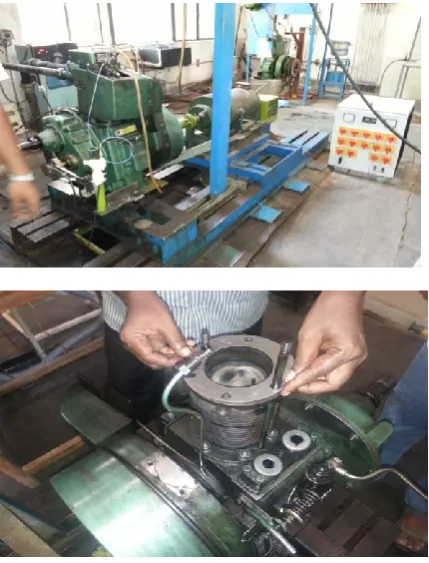
The engine used is a four stroke single cylinder, vertical, water cooled, natural aspirated, direct injection diesel engine. The specifications of the engine are given in table 1.
Table.1. Specifications of engine test rig.
A pressure transducer is used to monitor the injection pressure. The engine apparatus was interfaced with an emission measurement device AVL Digas 444 a five gas analyser, and also the setup is provided with necessary instruments for measuring combustion pressure and crank angle. These signals are interfaced to the computer through engine indicator for P-V and P-Ɵ diagrams with AVL INDIMICRA 602 –T10602A software version V2.5. Atmospheric air enters the intake manifold of the engine through an air filter and an air box. An air flow sensor fitted with the air box gave the input for the air consumption to the data acquisition system. All the inputs such as air and fuel consumption, engine brake power, cylinder pressure and crank angle were recorded by the data acquisition system, which is stored in the computer and displayed in the
S.no Component Specification
1 Make Kirloskar Engines
Ltd, Pune
2 Type of engine Four Stroke Single Cylinder Water Cooled Engine 3 Bore and Stroke 80 mm & 110 mm
4 Compression ratio 17.5 : 1
5 BHP and rpm 5.2kW & 1500 rpm
6 Fuel injection
pressure 200 N/m
2
7 Fuel injection
timing 27
0 BTDC
8 Specific fuel
consumption 0.25175 (kg/h)/kW
9 Dynamometer Eddy Current
Page | 329
monitor. A thermocouple in conjunction with a temperature indicator was connected at the exhaust pipe to measure the temperature of the exhaust gas. The smoke density of the exhaust was measured by the help of an AVL415 diesel smoke meter. A crank position sensor was connected to the output shaft to record the crank angle. The engine test rig is shown in figure 3 and the schematic diagram of experimental setup is given in figure 4.
Figure 3: Engine test rig
Figure 4. Schematic diagram of experimental setup
1. Engine 2. Dynamometer 3. Crank angle encoder 4. Load cell 5. Exhaust gas analyzer 6. Smoke meter 7. Control panel 8. Computer 9. Silencer
3. EXPERIMENTAL PROCEDURE
The engine used in this study was a direct injection single cylinder engine manufactured by Kirloskar. The engine was run at different compression ratios to evaluate the performance with emission charectaristics. Initially the engine was run on no load condition and its speed was maintained at a constant speed of 1500 rpm. The engine was tested at varying loads of 4.5 A, 9A, 13.5A and 18 A by means of an electrical dynamometer. For each loading conditions, the engine was run for at least 2 min after the data was collected. By changing the thickness of the cylinder head gasket the compression ratio can be changed to a certain limit. In order to vary the compression ratio of the engine in the present study, a thin copper spacer of 1 mm thick was inserted between the engine cylinder head and the cylinder block. With this various compression ratios of 13.7:1, 14.5:1, 15.37:1, 16.5:1 and 17.5:1 were obtained by using spacers apart from the standard compression ratio of 17.5:1.Matlab R2008a was used to assess the performance of diesel engine at these compression ratios and the graphs were generated.
4. RESULTS AND DISCUSSION
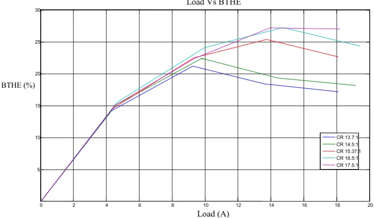
4.1 Brake thermal efficiency: Figure 5 shows the variation of brake thermal efficiency with load. The brake thermal efficiency with standard compression ratio of 17.5:1 was found to be 27.03% at full
load of 18A and brake thermal efficiency decreases as the compression ratio was reduced. This can be attributed that the fuel added to the cylinder which vaporizes and mixes with air to produce a fuel/air ratio distribution which is non uniform and 5 6
1
8
7 2
3
Page | 330
varies with time. This lead to the inferior
combustion at reduced compression ratio of 13.7:1.
Figure 5: Variation of Brake Thermal Efficiency w.r.t Load
4.2 Brake specific fuel consumption: An important parameter to measure the engine performance is the brake specific fuel consumption. Figure 6 shows the variation of BSFC with load at different compression ratios. In general, the BSFC decreases with the increase in load on engine. It was found from the figure that the BSFC was increased as the compression ratio was reduced. At higher compression ratio lesser value of BSFC is apparent because of better atomization which is associated with a marginal delay in admission of fuel due to high needle lift pressure during injection.
0 2 4 6 8 10 12 14 16 18 20
5 10 15 20 25 30
Load Vs BTHE
Load (A)
BTHE (%)
CR 13.7:1 CR 14.5:1 CR 15.37:1 CR 16.5:1 CR 17.5:1
0 2 4 6 8 10 12 14 16 18 20
0.25 0.3 0.35 0.4 0.45 0.5 0.55 0.6 0.65
0.7 Load Vs SFC
Load (A)
CR 13.7:1 CR 14.5:1 CR 15.37:1 CR 16.5:1 CR 17.5:1
Page | 331
Figure 6: Variation of Brake specific fuel consumption w.r.t Load
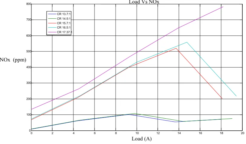
4.3 Nitric oxide emissions: Figure 7 shows the effect of NOx emissions wrt the compression by varying load. It is evident from the graph that as the compression ratio increases the NOx emissions also increases. This is due to the fact that the peak combustion pressure and temperature are high at higher compression ratios. Hence the NOx emissions are maximum at compression ratio of 17.5:1 and minimum at compression ratio of 13.7:1.
Figure 7: Effect of NOx emissions with varying compression ratio
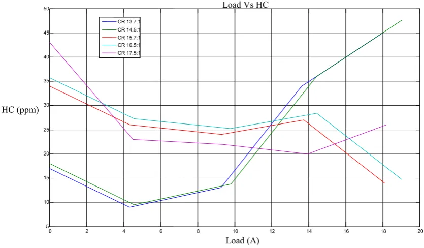
4.4 Hydro carbon emissions: Figure 8 shows the effect of varying compression ratio on hydrocarbon emissions. From the graph it is evident that the HC emission is deviant at various compression ratios.
0 2 4 6 8 10 12 14 16 18 20
0 100 200 300 400 500 600 700
800 Load Vs NOx
Load (A) NOx (ppm)
Page | 332
Figure 8: Effect of HC emissions with varying compression ratio
4.5 Carbon dioxide emissions: Figure 9 shows the effect of varying compression ratio on CO2
emissions. It is evident from the graph that CO2 emission is maximum at compression ratio of 16.5:1 and minimum at compression ratio of 13.7:1.
Figure 9: Effect of CO2 emissions with varying compression ratio
0 2 4 6 8 10 12 14 16 18 20
5 10 15 20 25 30 35 40 45
50 Load Vs HC
Load (A) HC (ppm)
CR 13.7:1 CR 14.5:1 CR 15.7:1 CR 16.5:1 CR 17.5:1
0 2 4 6 8 10 12 14 16 18 20
0.5 1 1.5 2 2.5 3 3.5 4 4.5 5
Load (A) CO2 (ppm)
Load Vs CO2
Page | 333
5. CONCLUSIONS
Experiments were conducted on diesel engine to analyse the performance at various compression ratios and Matlab was used to assess the performance of the engine and the graphs were generated.
REFERENCES
[1]Abou Al-Sood.M.M., Ibrahim.A.M., and Abdel Latif.A.A., 1999, “Optimum compression ratio variation of a 4-stroke, direct-injection diesel engine for minimum BSFC”, SAE Paper 1999-01-2519.
[2] Adnan Parlak, Halit Yasar and Bahri Sahin, 2003, “Performance and exhaust emission characteristics of a lower compression ratio LHR diesel engine”, Energy Conversion and Management, (44) pp. 163-175.
[3]Amjad Sheik, Shenbaga Vinayaga Moorthi.N, and Rudramoorthy.R., 2007, “Variable compression ratio engine: a future power plant for automobiles – an overview”, Proc. IMechE (221), pp. 1159-1168.
[4]Carlo Beatrice, Giovanni Avolio, Nicola Del Giacomo, and Chiara Guido, 2008,“Compression Ratio Influence on the Performance of an Advanced Single-Cylinder Diesel Engine Operating in Conventional and Low Temperature Combustion Mode”, SAE Technical Paper, 2008-01-1678, DOI:10.4271/2008-01-1678.
[5]Cenk Sayin, and Metin Gumus, 2011, “Impact of compression ratio and injection parameters on the performance and emissions of a DI diesel engine fueled with biodiesel-blended diesel fuel”, Journal of Applied Thermal Engineering 31 pp. 3182- 3188.
[6]Cursente.V,Pacaud.P, Gatellier.B, 2008, “Reduction of the Compression Ratio on a HSDI Diesel Engine : Combustion Design Evolution for
Compliance the Future Emission
Standards”, 0839 SAE International Journal of Fuels and Lubricants (1)1,pp.420-439, doi:10.4271/2008-01-0839.
[7]David.J., MacMillan, Theo Law, Paul.J., Shayler, and Ian Pegg, 2012, “The Influence of Compression Ratio on Indicated Emissions and Fuel Economy Responses to Input Variables for a D.I Diesel Engine Combustion System”, SAE Technical Paper , doi:10.4271/2012-01-0697.
[8]Helmantel.A., Gustavsson.J., and Denbratt.I., 2005, “Operation of DI diesel engine with variable effective compression ratio in HCCI and conventional diesel mode,” SAE 2005-01-0177.
[9]Heywood.J., 1988, “Internal
Combustion Engine Fundamentals”, New York, NY USA: McGraw-Hill.