Scholarship@Western
Scholarship@Western
Electronic Thesis and Dissertation Repository
8-22-2014 12:00 AM
The Doubly Adaptive LASSO Methods for Time Series Analysis
The Doubly Adaptive LASSO Methods for Time Series Analysis
Zi Zhen Liu
The University of Western Ontario
Supervisor Reg J. Kulperger
The University of Western Ontario Joint Supervisor Hao Yu
The University of Western Ontario
Graduate Program in Statistics and Actuarial Sciences
A thesis submitted in partial fulfillment of the requirements for the degree in Doctor of Philosophy
© Zi Zhen Liu 2014
Follow this and additional works at: https://ir.lib.uwo.ca/etd
Part of the Statistics and Probability Commons
Recommended Citation Recommended Citation
Liu, Zi Zhen, "The Doubly Adaptive LASSO Methods for Time Series Analysis" (2014). Electronic Thesis and Dissertation Repository. 2321.
https://ir.lib.uwo.ca/etd/2321
This Dissertation/Thesis is brought to you for free and open access by Scholarship@Western. It has been accepted for inclusion in Electronic Thesis and Dissertation Repository by an authorized administrator of
(Thesis format: Monograph )
by
Zi Zhen Liu
Graduate Program in Statistics and Actuarial Science
A thesis submitted in partial fulfillment
of the requirements for the degree of
Doctor of Philosophy
The School of Graduate and Postdoctoral Studies
The University of Western Ontario
London, Ontario, Canada
In this thesis, we propose a systematic approach called the doubly adaptive LASSO tai-lored to time series analysis, which includes four specific methods for four time series models, respectively:
ThePAC-weighted adaptive LASSO for univariate autoregressive (AR) models. Although the LASSO methodology has been applied to AR models, the existing methods in the literature ignore the temporal dependence information embedded in AR time series data. Consequently, the methods may not reflect the characteristics of underlying AR processes, especially, the lag order of AR models. The PAC-weighted adaptive LASSO incorporates the partial autocorrela-tion (PAC) into the adaptive LASSO weights. The PAC-weighted adaptive LASSO estimator has asymptotic oracle properties and a Monte Carlo study shows promising results.
ThePAC-weighted adaptive positive LASSO for autoregressive conditional heteroscedastic (ARCH) models. We have not found any results in the literature that apply the LASSO method-ology to ARCH models. The PAC-weighted adaptive positive LASSO incorporates the PAC information embedded in squared ARCH process into adaptive LASSO weights. The word
positivereflects the fact that the parameters in ARCH models are non-negative. We introduce a new concept named the surrogate of the second-order approximate likelihood, and propose a modified shooting algorithm to implement the PAC-weighted adaptive positive LASSO com-putationally. The PAC-weighted adaptive positive LASSO estimator has asymptotic oracle properties and a Monte Carlo study shows promising results.
The PLAC-weighted adaptive LASSO for vector autoregressive (VAR) models. Although the LASSO methodology has been applied to building VAR time series models, the existing methods in the literature ignore the temporal dependence information embedded in VAR time series data. Consequently, the methods may not reflect the characteristics of VAR time se-ries data, especially, the lag order of VAR models. The PLAC-weighted adaptive LASSO incorporates the partial lag autocorrelation (PLAC) into the adaptive LASSO weights. The PLAC-weighted adaptive LASSO estimator has oracle properties and Monte Carlo studies show promising results.
ThePLAC-weighted adaptive LASSO for BEKK vector ARCH (VARCH) models. We have not found any results in the literature that apply the LASSO methodology to VARCH processes. We focus on the BEKK VARCH models. The PLAC-weighted adaptive LASSO incorporates the PLAC information embedded in the squared BEKK VARCH process into the adaptive LASSO weights. We extend the concept of the surrogate of the second-order approximate like-lihood, and propose a modified shooting algorithm to implement the PLAC-weighted adaptive LASSO computationally. We conduct a Monte Carlo study and have preliminary results from the study.
weighted adaptive positive LASSO, PLAC-weighted adaptive LASSO, autoregressive, AR(P), autoregressive conditional heteroscedastic, ARCH(q), vector autoregressive, multivariate au-toregressive, VAR(p), vector ARCH, multivariate ARCH, VARCH(q), analytical score, analyt-ical Hessian, quadratic approximation, surrogate to approximate likelihood, S&P 500, Nikkei.
Mother Rangguo Liu
Father (Jinyuan Jia)
Brothers Jiabao Liu and Sanbao Liu
Sisters Jiaqiao Liu and (Jiayi Liu)
Wife Qingjun Zou
Daughters Dana Liu and Janet Liu
"Glory to God in the highest" (Luke 2:14 NIV)
I express my sincere gratitude to my supervisors Dr. Reg J. Kulperger and Dr. Hao Yu for their great support, encouragement, advice and guidance over the years of my doctoral re-search that have led to the completion of this dissertation. They suggested this interesting topic to me at the very start of my doctoral research. This dissertation would not have been possible without their initial suggestion of my research direction.
I thank very much the external examiner Dr. Zhou Zhou, and the examination committee members, Dr. Pei Yu, Dr. Ian McLeod, and Dr. Duncan Murdoch for reviewing my dissertation and offering valuable suggestions for improvement.
I thank the statistical community at the Department of Statistical and Actuarial Sciences of the University of Western Ontario. I learnt a lot from excellent lectures delivered by Dr. D. Bellhouse, Dr. W. J. Braun, Dr. W. He, Dr. R. J. Kulperger, Dr. I. McLeod, Dr. D. Murdoch, Dr. S. Provost, and Dr. H. Yu. Thanks also go to Ms. J. Bai and Ms. J. Dungavell for their logistic support.
I express my sincere gratitude to Dr. Nancy Reid for bringing me into the field of statistics by hiring me as a research assistant under her supervision. I thank the statistical community at the Department of Statistical Sciences of the University of Toronto. I learnt a lot from excellent lectures delivered by Dr. D. Brenner, Dr. M. Evans, Dr. A. Feuerverger, Dr. D. A. S. Fraser, and Dr. K. Knight, Dr. P. McDunnough, Dr. R. M. Neal, Dr. N. Reid, Dr. J. S. Rosenthal, Dr. J. Stafford, and Dr. F. Yao.
I express my deep love to my mother Rangguo Liu and my father (Jinyuan Jia) for their unfathomable, absolute and unqualified love to me. I express my deep love to my brothers and sisters Jiabao Liu, Jiaqiao Liu, (Jiayi Liu), and Sanbao Liu for their love, kindness, encourage-ment and help in my life. I express my deep love to my wife Qingjun Zou and my daughters Dana Liu and Janet Liu for their sacrifice and support during my extremely busy years of re-search.
Zi Zhen Liu
July 18, 2014
London, Ontario, Canada
Abstract i
Dedication iii
Acknowlegements iv
List of Figures viii
List of Tables x
List of Appendices xii
1 Introduction 1
1.1 Parsimonious models and shrinkage . . . 1
1.2 The LASSO methodology . . . 3
1.2.1 The shrinkage mechanism . . . 4
1.2.2 The computational algorithms . . . 7
1.2.3 The asymptotic properties . . . 9
1.2.4 Selection consistency and irrepresentable conditions . . . 10
1.2.5 The adaptive LASSO and its oracle properties . . . 12
1.2.6 Critiques for the oracle properties . . . 15
1.3 Literature review of the LASSO methodology in time series analysis . . . 17
1.4 The doubly adaptive LASSO for time series models . . . 20
1.4.1 Motivation . . . 20
1.4.2 The doubly adaptive LASSO (daLASSO) . . . 21
1.4.3 Determining optimal values for tuning and weighting parameters . . . . 22
1.5 Thesis organization . . . 23
2 The Doubly Adaptive LASSO for AR(p) Models 25 2.1 Introduction . . . 25
2.2 The AR(p) process and standard modelling procedure . . . 26
2.3 The adaptive and doubly adaptive LASSO . . . 28
2.3.1 The doubly adaptive LASSO when p is unknown . . . 29
2.3.2 The adaptive LASSO when p is known . . . 31
2.4 Asymptotic properties of the doubly adaptive LASSO . . . 31
2.5 Computation algorithms for the doubly adaptive LASSO . . . 41
weighting parameters using samples of different sizes . . . 45
2.6.2 Performance of the daLASSO with tuning and weighting parameters being chosen via LOOCV using a sample of moderate size . . . 47
2.7 Real data analysis . . . 51
2.7.1 Chemical process time series . . . 51
2.7.2 Annual tree ring width . . . 51
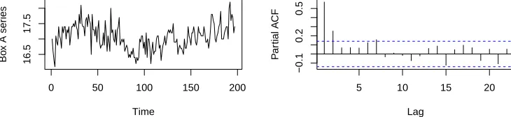
2.7.3 Annual sunspot numbers . . . 54
3 The Doubly Adaptive Positive LASSO for ARCH(q) Models 55 3.1 Introduction . . . 55
3.2 The pure ARCH(q) process and standard modelling procedure . . . 57
3.3 The adaptive and doubly adaptive positive LASSO . . . 59
3.3.1 The doubly adaptive positive LASSO when q is unknown . . . 59
3.3.2 The adaptive positive LASSO when q is known . . . 62
3.4 Asymptotic properties of the doubly adaptive positive LASSO . . . 62
3.5 Computation algorithm for the doubly adaptive positive LASSO . . . 72
3.5.1 Quadratic approximation to the negative log quasi likelihood . . . 73
3.5.2 The surrogate of the quadratic approximation of likelihood . . . 74
3.5.3 The modified shooting algorithm . . . 75
3.6 Monte Carlo study . . . 78
3.7 Real data analysis examples: models for stock indices . . . 81
3.7.1 The US S&P500 Return Data . . . 81
3.7.2 The Japan Nikkei Return Data . . . 82
4 The Doubly Adaptive LASSO for Multivariate AR(p) Models 86 4.1 Introduction . . . 86
4.2 The VAR(p) process and standard modelling procedure . . . 87
4.3 The adaptive LASSO and doubly adaptive LASSO . . . 90
4.3.1 The doubly adaptive LASSO when p is unknown . . . 91
4.3.2 The adaptive LASSO when p is known . . . 95
4.4 The asymptotic properties of the doubly adaptive LASSO . . . 95
4.5 Computation algorithm for the doubly adaptive LASSO . . . 104
4.6 Monte Carlo study . . . 105
4.6.1 A bivariate VAR(5) process . . . 106
4.6.2 A trivariate VAR(5) process . . . 108
4.7 Real data analysis . . . 111
5 The Doubly Adaptive LASSO for BEKK Multivariate ARCH(q) models 116 5.1 Introduction . . . 116
5.2 The BEKK VARCH(q) model and standard modelling procedure . . . 117
5.3 The adaptive and doubly adaptive LASSO . . . 120
5.3.1 The adaptive LASSO when q is known . . . 120
5.3.2 The doubly adaptive LASSO when q is unknown . . . 121
5.4.2 The surrogate of the quadratic approximation of likelihood . . . 125
5.4.3 The modified shooting algorithm . . . 126
5.5 Monte Carlo study . . . 128
6 Discussion and Future Work 133 A Some Definitions and Theorems in Probability 136 A.1 Stationarity . . . 136
A.2 White Noise . . . 137
A.3 Ergodicity . . . 138
A.4 Martingale Difference . . . 138
A.5 Stochastic Boundedness . . . 139
B Some Definitions and Formulae in Matrix Calculus 140 C The Partial Lag Autocorrelation Matrix Function 143 C.1 Autocorrelation Matrix Function . . . 143
C.2 Partial Lag Autocorrelation Matrix . . . 145
C.3 Partial Autoregression Matrix Function . . . 149
C.4 Recursive Algorithm . . . 152
C.5 Estimation and Inference . . . 156
D Analytical Score and Hessian for BEKK VARCH(q) Model 158 D.1 The Negative Log Quasi-likelihood of BEKK VARCH(q) Models . . . 158
D.2 The Negative Score Gradient . . . 158
D.2.1 Derivation of∂log|HHHt|/∂hhh0t and∂(yyyt0HHH−t1yyyt)/∂hhh0t . . . 159
D.2.2 Derivation of∂hhht/∂θθθ0 . . . 159
D.2.3 Derivation ofssst(θθθ) . . . 160
D.3 The Analytical Hessian Matrix . . . 161
D.3.1 Derivation of∂QQQ0t/∂θθθ0 . . . 161
D.3.2 Derivation of∂vecRRRt−1/∂θθθ0 . . . 162
Bibliography 164
1.1 (a) Illustration of (1.11); (b) Illustration of the LASSO estimator in the or-thonormal design. . . 5 1.2 The shooting algorithm (Fu, 1998). . . 9 1.3 Illustration of the adaptive LASSO estimator in the orthonormal design with
the adaptive weight ˆwjbeing 1/|βˆolsj |γ. . . 14 2.1 Empirical distributions of the doubly adaptive LASSO estimates for the AR order as sample
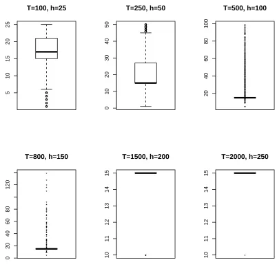
size increases, based on 10,000 replications (10,000 data sets for each of 6 different sample sizes were generated formYt=0.2Yt−1+0.1Yt−3+0.2Yt−5+0.2Yt−10+0.25Yt−15+at. Setγ0= 4.5,γ1=5, andγ2=1.5. The optimal value ofλT was chosen by theCp.) . . . 48
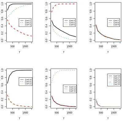
2.2 Empirical probabilities of AR coefficients being selected in the model by the doubly adaptive LASSO for as sample size increases, based on 10,000 replications (10,000 data sets for each of 6 different sample sizesT=100,250,500,800,1500,2000 were generated formYt=0.2Yt−1+ 0.1Yt−3+0.2Yt−5+0.2Yt−10+0.25Yt−15+at. Seth=25,50,100,150,200,250 accordingly with
respect to the different T. Setγ0=4.5, γ1=5, andγ2=1.5. The optimal value ofλT was
chosen by theCp.) . . . 49
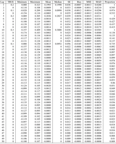
2.3 Chemical process time series (Data source: Box et al. 2004) . . . 53 2.4 Annual tree ring width measurements on Douglas fir (1194-1964) (Data source: McLeod
and Hipel, 1995) . . . 53 2.5 Annual sunspots numbers (1700-2011) (Data source: SIDC website
http://sidc.be/sunspot-data/) . . . 54 3.1 The modified shooting algorithm for the doubly adaptive positive LASSO.
Left: Estimate for θj is 0. Right: S0,j<−λj, the intersection of Sj and −λj
yields a positive estimate forθj. . . 76
3.2 The S&P500 Daily Returns and Squared Daily Returns from January 2, 1990 to Jan-uary 22, 2009. Data source: Yahoo Finance . . . 82 3.3 The ACF of S&P500 Daily Returns and Squared Daily Returns from January 2, 1990
to January 22, 2009 . . . 83 3.4 The Nikkei Daily Returns and Squared Daily Returns from January 2, 1990 to January
22, 2009. Data source: Yahoo Finance . . . 84 3.5 The ACF of Nikkei Daily Returns and Squared Daily Returns from January 2, 1990 to
January 22, 2009. Data source: Yahoo Finance . . . 85 4.1 Quarterly West German investment, income, and consumption data (1960-1982)
(Lütke-pohl, 2006, p. 77 – 79) . . . 114
2.1 Empirical statistics of the doubly adaptive LASSO estimates for the AR order, based on 10,000 replications (10,000 data sets each of size T=2,000 were generated fromYt=0.2Yt−1+ 0.1Yt−3+0.2Yt−5+0.2Yt−10+0.25Yt−15+at. Seth=250. Setγ0=4.5,γ1=5, andγ2=1.5. Use theCpto choose the value ofλT.) . . . 46
2.2 Empirical statistics of the doubly adaptive LASSO estimates for the AR coefficients, based on 10,000 replications (10,000 data sets each of size T=2,000 were generated fromYt=0.2Yt−1+ 0.1Yt−3+0.2Yt−5+0.2Yt−10+0.25Yt−15+at. Seth=250. Setγ0=4.5,γ1=5, andγ2=1.5. Use theCpto choose the value ofλT.) . . . 46
2.3 Empirical statistics of the adaptive LASSO estimates for the AR order, based on 1,000 replica-tions (1,000 data sets each of size T=800 were generated fromYt=0.2Yt−1+0.1Yt−3+0.2Yt−5+ 0.2Yt−10+0.1Yt−15+at(Nardi, 2011). Seth=50,γ0=γ2=0. The optimal value ofγ1was chosen by the LOOCV and the optimal value ofλT chosen by theCp) . . . 50
2.4 Empirical statistics of the doubly adaptive LASSO estimates for the AR order, based on 1,000 replications (1,000 data sets each of size T=800 were generated fromYt=0.2Yt−1+0.1Yt−3+ 0.2Yt−5+0.2Yt−10+0.1Yt−15+at(Nardi, 2011). Seth=50. The optimal values ofγ0,γ1, and
γ2were chosen by the LOOCV and the optimal value ofλT chosen by theCp) . . . 50
2.5 Empirical statistics of the doubly adaptive LASSO estimates for the AR coefficients, based on 1,000 replications (1,000 data sets each of size T=800 were generated fromYt=0.2Yt−1+ 0.1Yt−3+0.2Yt−5+0.2Yt−10+0.1Yt−15+at(Nardi, 2011). Seth=50. The optimal values ofγ0,
γ1, andγ2were chosen by the LOOCV and the optimal value ofλT chosen by theCp) . . . . 52
3.1 Empirical statistics of the doubly adaptive positive LASSO estimates for the ARCH order, based on 764 replications each of size T=1,000 generated from the model (3.24). The BIC was used to choose (λT,γ0,γ1,γ2) . . . 79
3.2 Empirical statistics of the doubly adaptive positive LASSO estimates for the ARCH coeffi-cients, based on 764 replications each of size T=1,000 generated from the model (3.24). The
BIC was used to choose (λT,γ0,γ1,γ2) . . . 80
4.1 Empirical statistics of the doubly adaptive LASSO estimates for the bivariate AR order based on 1,000 replications each of size T=2,000, generated from bivariate AR(5) model with
coef-ficients defined in (4.30). Set h=10. Use the BIC to chooseλ,γ0,γ1, andγ2. . . 108
4.2 Empirical distribution of the doubly adaptive LASSO estimates for the bivariate AR order based on 1,000 replications each of size T=2,000, generated from the bivariate AR(5) model with coefficients defined in (4.30). Set h=10. Use the BIC to chooseλ,γ0,γ1, andγ2. . . 108
4.3 Empirical statistics of the doubly adaptive LASSO estimates for the bivariate AR coefficients
Φ
ΦΦ111−ΦΦΦ555 based on 1,000 replications each of size T=2,000, generated from bivariate AR(5) model with coefficients defined in (4.30). Set h=10. Use the BIC to chooseλ,γ0,γ1, andγ2. . 109
ficients defined in (4.32). Set h=10. Use the BIC to chooseλ,γ0,γ1, andγ2. . . 111
4.5 Empirical distribution of the doubly adaptive LASSO estimates for the bivariate AR order based on 1,000 replications each of size T=2,000, generated from bivariate AR(5) model with
coefficients defined in (4.32). Set h=10. Use the BIC to chooseλ,γ0,γ1, andγ2. . . 111
4.6 Empirical statistics of the doubly adaptive LASSO estimates for the bivariate AR coefficients
Φ
ΦΦ111−ΦΦΦ555 based on 1,000 replications each of size T=2,000, generated from bivariate AR(5) model with coefficients defined in (4.32). Set h=10. Use the BIC to chooseλ,γ0,γ1, andγ2). See Table 4.7 forΦΦΦ666−ΦΦΦ10. . . 112
4.7 Empirical statistics of the doubly adaptive LASSO estimates for the VAR coefficientsΦΦΦ666−
Φ
ΦΦ10 based on 1,000 replications each of size T=2,000, generated from VAR(5) model with coefficients defined in (4.32). Set h=10. Use the BIC to chooseλ,γ0,γ1, andγ2). See Table 4.6 forΦΦΦ111−ΦΦΦ5. . . 113
5.1 Empirical distribution of the doubly adaptive LASSO estimates for the trivariate BEKK ARCH(2) order based on 25 convergent replications each of size T=1,000, generated from trivariate BEKK ARCH(2) model with coefficients defined in (5.25). Set h=4. Use the BIC to chooseλ,
γ0,γ1, andγ2. . . 131
5.2 Empirical statistics of the doubly adaptive LASSO estimates for the trivariate BEKK ARCH(2) order based on 25 convergent replications each of size T=1,000, generated from trivariate
BEKK ARCH(2) model with coefficients defined in (5.25). Set h=4. Use the BIC to chooseλ,
γ0,γ1, andγ2. . . 131
5.3 Empirical statistics of the doubly adaptive LASSO estimates for the trivariate ARCH coeffi-cientsCCC,AAA111andAAA222based on 25 convergent replications each of size T=1,000, generated from
trivariate ARCH(2) model with coefficients defined in (5.25). Set h=4. Use the BIC to choose
λ,γ0,γ1, andγ2. . . 132
Appendix A Some Definitions and Theorems in Probability . . . 136
Appendix B Some Definitions and Formulae in Matrix Calculus . . . 140
Appendix C The Partial Lag Autocorrelation Matrix Function . . . 143
Appendix D Analytical Score and Hessian for BEKK VARCH(q) Model . . . 158
Introduction
1.1
Parsimonious models and shrinkage
A large number of statistical models have linear structure. Say we have a data set with
xi1, · · ·,xip being the inputs and yi the outcome. The models with linear structure have the form
f(E[yi|xxxi])=β1x1+· · ·+βpxp, (1.1)
where the inputxi j can be continuous, binary, or categorical, and f would have different func-tional forms depending on whether we have a classification or regression problem. If yi is continuous, we often use the identity function for f, which is the linear regression model. Ifyi
is binary, we often use the logit function for f, which is the logistic regression model. Ifyiis
the number of occurrence of a rare event, we often use the Poisson regression model with the log function for f. Ifyiis the hazard rate, we often use the log function for f, which is the Cox proportional hazard model. What is common in all these models is that they are all linear in the inputsxi1, · · ·,xip. There are good reasons for these linear-structured models to be widely used. First, they are simple in functional structure and thus more interpretable than complex nonlinear models. Moreover, they often provide an adequate description of how the inputs af-fect the output. Finally, they sometimes outperform more complicated nonlinear models with regard to prediction.
When we fit the model to the data, we are not always satisfied with the full model, especially when the number of the inputs is large. The so-called subset selection or variable selection
procedures eliminate the insignificant variables from the model while keeping those significant
ones in the model. We need parsimonious models for two reasons. The first is prediction accuracy. Prediction accuracy may be improved by excluding insignificant variables although the bias of estimators may be increased by doing so. With the full model, the estimators for the parameters have lower bias but larger variance. In contrast, for a parsimonious model, the estimators may have larger bias but smaller variance. We would like to sacrifice a little bit of bias but reduce the prediction variance with the net benefit of reduced mean squared error of prediction. This is the so-called the bias-variance tradeoff. The second reason for parsimonious models is the ease ofinterpretation. From a smaller model it is easier for us to see the inputs that have the strongest effects on the outcome.
Variable selection is a crucial but difficult problem in building statistical models. A large amount of research has been and continues to be devoted to this topic. There are a variety of subset selection strategies in the literature. (i) The best subset selection fits models of all possible subsets, then puts these models into categories corresponding to 0,1,· · ·,pparameter models, then selects one from each category by minimal residual sum of squares which results in p+1 candidate models that contain 0,1,· · ·,p variables, respectively, and finally chooses the model that satisfies some optimal criterion, say, the Akaike Information Criterion (AIC). This approach is feasible for moderate p. (ii) The forward Stepwiseselection starts with the intercept, then sequentially adds into the model the variable that most improves the fit to yield
p+1 nested candidate models, and finally chooses the model that satisfies the some optimal criterion like the AIC. (iii) The backward Stepwise selection starts with the full model, and sequentially removes the least significant variables. (iv) Theforward stagewiseselection starts with an intercept equal to ¯y, and includes the next variable that is most correlated with the current residual. The process continues until none of the variables have correlation with the current residuals and the final model is obtained.
Subset selection procedures are discrete in the sense that variables are either retained or discarded. They often have high variability (Breiman, 1996). Apart from instability issue they quickly become computationally infeasible as p becomes large. Methods using shrinkage,
penalization problem for the model (1.1) has the general form
ˆ
βββ=arg min βββ
n
X
i=1
`((yi,xxxi),βββ)+λnP(βββ), (1.2)
where `(yi,xxx0iβββ) is a convex loss function, P(βββ) is a penalty function, λn> 0 is the tuning
parameter. Depending on the functional form of f in (1.1) there are many loss function, for example, the square error loss in linear regression, the negative log-likelihood in generalized linear models, the negative partial log-likelihood function in Cox proportional hazards model, and etc. The tuning parameter λn balances the loss and the penalty. It determines the
bias-variance tradeoffby controlling the amount of penalty. A variety of penalty functions has been proposed in the literature. An example is theBridgepenalty function of Frank and Friedman (1993) defined as
P(βββ)=
p
X
j=1
|βj|γ, (1.3)
whereγ≥0. While they did not solve for the Bridge estimator, Frank and Friedman pointed out that it is desirable to get the optimal value of γ. The Bridge penalty includes a few well known penalty functions as special cases. Forγ=0, P(βββ) reduces to many well-known model
selection criteria such as the Akaike Information criterion (AIC) and the Bayesian Information criterion (BIC). For γ ∈(0,1], P(βββ) is known as the soft-thresholding penalty (Donoho and Johnstone, 1994). Particularly for γ =1, it is the penalty for the least absolute shrinkage and selection operator (LASSO) (Tibshirani, 1996). Forγ=2, it is the penalty for theridge regression(Hoerl and Kennard, 1970).
In this dissertation, we focus on the the LASSO methodology only. We adapt the LASSO to the context of time series analysis and propose a doubly adaptive LASSO methodology for time series models.
1.2
The LASSO methodology
algorithms. In this section, we review the definition, asymptotic properties, algorithms, and the irrepresentable condition, and the adaptive version of the LASSO.
1.2.1
The shrinkage mechanism
Consider the linear regression model, yi= xxxiβββ+i, where 1,· · ·,n are iid(0, σ2). Let xxxi =
(x1, · · ·, xp)0andβββ=(β1, · · ·, βp).
Definition (The LASSO(Tibshirani, 1996)). The LASSO estimator, denoted by ˆβββLn, is defined as
ˆ
βββLn=arg min βββ
n
X
i=1
(yi−xxx0iβββ)2+λn p
X
j=1
|βj|, (1.4)
or, equivalently,
ˆ
βββnL=arg min βββ
n
X
i=1
(yi−xxx0iβββ)2 subject to
p
X
j=1
|βj| ≤t.
There is no closed form formula for ˆβββnL in general. However, for the special case of the orthonormal design, an analytical formula exists, and we record it here as a proposition, which may shed light on our intuitive understanding of the shrinkage mechanism of the LASSO.
Proposition 1.2.1 (The LASSO estimator in orthonormal design (Tibshirani, 1996)). For
the orthonormal design in which Pn
i=1xxxixxx
0
i = I with I being the identity matrix, the LASSO
estimator (1.4) is a function ofλn>0in the form
ˆ βL
j(λn)=
|βˆolsj | −λn
2
+
sgn( ˆβolsj ), (1.5)
for j=1, · · ·, p where(z)+=max{z, 0}and sgn(z)= +1,0,−1if z>0,=0,<0, respectively. Also t is a function ofλndefined by
t(λn)=
p
X
j=1
|βˆolsj | −λn
2
+
. (1.6)
To get the results of Proposition 1.2.1, note that for the orthonormal design, Pn i=1(yi−
xxx0iβββ)2=Pn
i=1(yi−yˆi)2+
Pp
j=1(βj−βˆ
ols j )
2, where ˆβols
forβj and ˆyi is the OLS predicted value. Applying the Karush-Kuhn-Tucker (KKT) theorem
for the constrained optimization problem1, we have
(a) ˆβLj−βˆols
j +
λn
2sgn( ˆβLj)=0, j=1, · · ·, p,
(b) λn≥0,
(c) λn(Ppj=1|βˆLj| −t)=0,
(d) Pp
j=1|βˆ
L
j| ≤t<∞.
(1.7)
Consider the two cases. In the first case,λn=0. Then from (1.7)(a) we have ˆβLj =βˆolsj so that
from (1.7)(d) we have Pp
j=1|βˆ
ols
j | ≤t<∞, which is not true because ˆβ ols
j is the unconstrained
minimizer.
- βˆols j 6
ˆ βL
j
@ @
@ @
@@ @
@ @ @ @ @
|βˆL
j|=|βˆ ols
j | −λn/2
λn
2
−λn
2
(a)
- βˆols j 6
ˆ βL
j
|βˆLj|=|βˆolsj | −λn/2
sgn( ˆβLj)=sgn( ˆβolsj ) λn
2
−λn
2
λn
2
(b)
Figure 1.1: (a) Illustration of (1.11); (b) Illustration of the LASSO estimator in the orthonormal design.
Now consider the second case in whichλn>0. From (1.7)(c) we have p
X
j=1
|βˆLj|=t. (1.8)
We write (1.7)(a) as|βˆL
j|sgn( ˆβ L j)=|βˆ
ols j |sgn( ˆβ
ols j )−
λn
2sgn( ˆβLj) or
|βˆLj|=|βˆolsj |sgn( ˆβLj)sgn( ˆβolsj )−λn
2. (1.9)
The LHS of (1.9) is non-negative. For the RHS of (1.9) to be non-negative, it is necessary that
sgn( ˆβLj)=sgn( ˆβolsj ), (1.10)
1Karush-Kuhn-Tucker theorem(Chong and Zak, 2008, p.458): Let f,ggg,hhh∈C1. Letxxx∗be a regular point
and a local minimizer for the problem of minimizingfsubject tohhh(xxx)=000 andggg(xxx)≤000 wheref:Rn→
R,hhh:Rn→ Rm(m<n) andggg:Rn→Rp. Then there existλλλ∗1∈Rmandλλλ
∗
2∈Rpsuch that (a)D f(xxx
∗)+λλλ∗0
1hhh(xxx
∗)+λλλ∗0
2ggg(xxx
∗)=0000,
so that
|βˆLj|=|βˆolsj | −λn
2 . (1.11)
With pictorial aid it is easy to find the solution. Figure 1.1(a) is the plot of (1.11) whereas Figure 1.1(b) is the plot of (1.5) because it satisfies both (1.10) and (1.11). Substituting the ˆβLj into (1.8) we have (1.6).
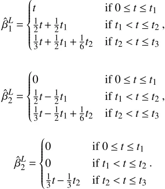
Proposition 1.2.1 gives us insight into the shrinkage mechanism of the LASSO. From Fig-ure 1.1(b) we see clearly that the lasso shrinkage causes the estimates of the non-zero coeffi -cients to be biased towards zero. We also see that the LASSO translates each coefficient by a constant factor λn/2, truncating at zero, which is known assoft thresholding (Donoho and
Johnstone, 1994). The LASSO also performscontinuous subset selection. Let us look at a sim-ple examsim-ple. Suppose that we have three standardized and orthonormal input variables x1,x2
andx3. We assume that ˆβols1 >βˆols2 >βˆols3 >0. We make use of Proposition 1.2.1. Ifλn≥2 ˆβols1 ,
we have ˆβLj =0, for j=1,2,3, andt=0. If 2 ˆβols2 ≤λn<2 ˆβols1 , we have ˆβL1=βˆols1 −λn/2, ˆβLj =0 for j= 2,3, and 0<t ≤βˆ1ols−βˆols2 ,t1. If 2 ˆβols3 ≤λn< 2 ˆβols2 , we have ˆβLj = βˆolsj −λn/2 for
j=1,2 ˆβL3=0, andt1<t≤βˆols1 +βˆols2 −2 ˆβols3 ,t2. If 0≤λn<2 ˆβols3 , we have ˆβLj =βˆolsj −λn/2 for
j=1,2,3 , andt2<t≤βˆols1 +βˆols2 +βˆols3 ,t3. A bit of mechanical manipulation and rearranging
gives us the following solution
ˆ βL
1=
t if 0≤t≤t1 1
2t+ 1
2t1 ift1<t≤t2
1 3t+
1 2t1+
1
6t2 ift2<t≤t3
,
ˆ βL
2=
0 if 0≤t≤t1
1 2t−
1
2t1 ift1<t≤t2
1 3t−
1 2t1+
1
6t2 ift2<t≤t3
,
ˆ βL
2 =
0 if 0≤t≤t1
0 ift1<t≤t2
1 3t−
1
3t2 ift2<t≤t3
.
1.2.2
The computational algorithms
The LASSO procedure has an attractive property in terms of optimization. The objective func-tion to be minimized is convex. Thus it does not suffer from the issue of multiple local minimal points, and the global minimum problem can be solved efficiently using a variety of algo-rithms, including but not limited to the quadratic programming for the LASSO (Tibshirani, 1996), the shooting algorithm for the LASSO (Fu, 1998), the homotopy algorithm for the LASSO (Osborne, Presnell and Turlach, 2000a, 2000b), the least angle regression and shrink-age (LARS) (Efron, Hastie, Johnston, and Tibshirani, 2004), the coordinate descent algorithm for the LASSO (Friedman, Hastie, Hoefling and Tibshirani, 2007). Note that in principle, the shooting algorithm belongs to the class of coordinate descent algorithms. The LARS belongs to the class of continuation methods or homotopy methods. That is why we put the definite articlethebefore the name of each algorithm.
In this dissertation, we make use of the LARS algorithm of Efron, et al (2004). We also modify the shooting algorithm of Fu (1998) to minimize the LASSO regularized negative likeli-hood functions in Chapter 3 and Chapter 5 . Here we briefly review the LARS and the shooting algorithms.
The LARS algorithm
Perhaps the LARS algorithm (Efron, et al 2004) is the most well-known continuation algorithm in data mining. The LARS gives path solutions and the path is piece-wise linear, It is contrived with great ingenuity2. It is also extremely efficient so that the computational cost of the entire steps is of the same order as that of the ordinary least squares solution for the full model. See Algorithm 1 for details.
2In the preface to the bookThe Science of Bradley Efron: Selected Papers(Edited by Morris and Tibshirani),
Algorithm 1:Least angle regression for the LASSO (Hastie, et al, 2009, p.74 - 76).
1 Standardize the predictors to have mean zero and unit norm. Start with the residual
rrr=yyy−yyyˆ,β1, · · ·, βp=0
2 Find the predictorxjmost correlated withrrr.
3 Moveβjfrom 0 towards its least-squares coefficient , until some other competitor
< xxxj,rrr>has as much correlation with the current residual as does xj.
4 Moveβjandβkin the direction defined by their joint least squares coefficient of the
current residual on (xxxj,xxxk), until some other competitorxxxlhas as much correlation with the current residual.
5 If a non-zero coefficient hits zero, drop its variable from the active set of variables and
recompute the current joint least squares direction.
6 Continue in this way until all ppredictors have been entered. After min(n−1,p) steps,
we arrive at the full least-squares solution.
The shooting algorithm
Fu (1998) proposed a shooting algorithm for solving the LASSO problem numerically. Let
Q(βββ) = (yyy−XXXβββ)0(yyy−XXXβββ), where yyy= (y1, · · ·, yn)0, and XXX is the design matrix. Then the
LASSO estimator for the linear regression model is to minimize the objective functionQ(βββ)+
λPp
j=1|βj|. The first order necessary condition of optimization is∂Q(βββ)/∂βββ=−λsgn(βββ), and
∂Q(βββ)/∂βββ=−2XXX0(yyy−XXXβββ)=2XXX0Pp
i=1xxx
iβ i−2XXX
0
yyy, which is the vector
2Pp
i=1(xxx 1)0
xxxiβi−2(xxx1)0yyy
... 2Pp
i=1(xxx
j)0xxxiβ
i−2(xxxj)
0
yyy
... 2Pp
i=1(xxx
p)0xxxiβ
i−2(xxxp)
0 yyy =
2(xxx1)0xxx1β1+2P
i,1(xxx
1)0xxxiβ
i−2(xxx1)
0
yyy
... 2(xxxj)0xxxjβj+2Pi,j(xxx
j)0xxxiβ
i−2(xxxj)
0
yyy
... 2(xxxp)0xxxpβp+2Pi,p(xxx
p)0xxxiβ
i−2(xxxp)
0 yyy , S1 ... Sj ... Sp ,
withxxxj=(x1j,· · ·,xn j)0 being the jth column ofXXX. Letting
S0,j=S0(0,βββ(−j),XXX,yyy)=2X
i,j
(xxxj)0xxxiβi−2(xxxj)0yyy,
whereβββ(−j) is the coefficient vector withoutβj, we have
Sj=Sj(βββ,XXX,yyy)=2(xxxj)0xxxjβj+S0,j,
for j=1, · · ·,p.
λ
−λ
r ˆ βj
S0
βj
Sj
λ
−λ
Sj
r
S0
βj
λ
−λ
r ˆ βj
Sj S0r
βj
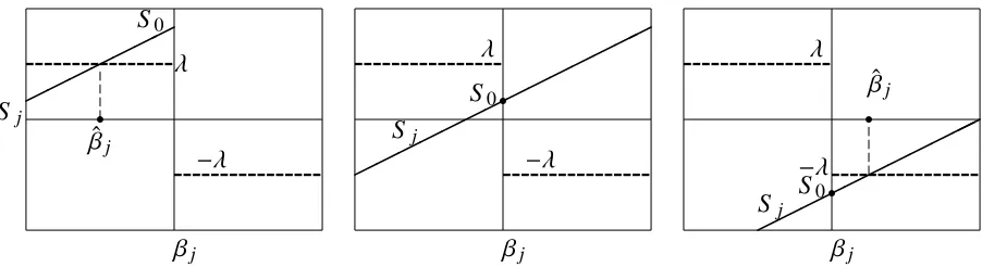
Figure 1.2: The shooting algorithm (Fu, 1998).
or right figure, the unique non-zero solution is obtained. The solution is expressible in closed form as
ˆ βj=
λ−S0,j
2(xxxj)0xxxj if S0,j> λ,
0 if |S0,j|< λ,
−λ−S0,j
2(xxxj)0xxxj if S0,j<−λ,
for j=1, · · ·, p.
1.2.3
The asymptotic properties
Knight and Fu (2000) set up a paradigm for asymptotic analysis of the whole class of Bridge estimator defined in (1.2) and (1.3) with the loss being the squared error loss, including the LASSO estimator. We follow Knight and Fu to conduct the asymptotic analysis. So we quote the following theorems from Knight and Fu (2000).
Consider the linear regression model, yi = xxxiβββ+i, where 1,· · ·,n are iid(0, σ2) with
regularity conditions for the design:
A1:CCCn= 1nPT
i=1xxxixxx
0
i → CCC withCCC being a positive definitep×pmatrix, A2: 1nmax1≤i≤nxxx0ixxxi → 0, asn→ ∞.
Theorem 1.2.2 (Consistency (Knight and Fu, 2000)). Under A1and A2, if λn/n→λ0≥0
then
ˆ
βββLn−→P argmin βββ (
Z(βββ)),
where
Z(βββ)=(βββ−βββ∗)0CCC(βββ−βββ∗)+λ0
p
X
j=1
|βj|.
Theorem 1.2.3 (√n-Consistency (Knight and Fu, 2000)). Under A1and A2, if λn/√n→
λ1≥0then
√
n( ˆβββLn−βββ∗)−→D argmin
u uu
(V1(uuu)),
where
V1(uuu)=−2uuu0www+uuu0CCCuuu+λ1
p
X
j=1
n
ujsgn(βj)I(βj,0)+|uj|I(βj=0)o.
and www ∼ N(000,σ2CCC))).
Remarks:
(i) By Theorem 1.2.2, ifλ0=0, then argmin(Z(βββ))=βββ∗and so ˆβββ
L
n is consistent.
(ii) By Theorem 1.2.3, ifλn=O(
√
n), then ˆβββLn is √n-consistent. (iii) By Theorem 1.2.3, ifλ1=0, then
√
n( ˆβββLn−βββ∗) has the same asymptotic distribution as does √n( ˆβββolsn −βββ∗).
(iv) From Theorem 1.2.3, we see that ifλ1>0, the non-zero parameters are estimated with
some asymptotic bias.
1.2.4
Selection consistency and irrepresentable conditions
Estimation consistency does not necessarily imply selection consistency. Without loss of generality, suppose that β1, · · ·, βr , 0 and βr+1, · · ·, βp = 0. Let S ={1,2, · · ·, r}. Let Sc={r+1, · · ·, p}. Let ˆSn={j: ˆβLj,n,0}. Let ˆScn={j: ˆβLj,n=0}. LetβββS=(β1, · · ·, βr)
0. We rewrite the the matrixCCC as follows
C
CCSS CCCSSc
CCCSSc CCC ScSc
!
,
whereCCCSS isr×rmatrix,CCCSc
Definition (Selection consistency (Zou, 2006)). The LASSO variable selection is consistent if and only if limnP( ˆSn=S)=1.
Proposition 1.2.4 . UnderA1andA2, ifλn/
√
n→λ1>0then
lim inf
n P( ˆS c
n=Sc)=c>0.
Proposition 1.2.4 is summarized from a result of Knight and Fu (2000). For the proof, see the paragraph before Example 1 in the paper of Knight and Fu (2000). Proposition 1.2.4 says that when some ofβj’s are exactly 0, the limiting distribution specified in Theorem 1.2.3 of the
LASSO estimator puts positive probability at 0 ifλn=O(
√
n).
Proposition 1.2.5 (Zou, 2006). UnderA1andA2, ifλn/√n→λ1≥0then
lim sup
n
P( ˆSn=S)≤c<1.
Proposition 1.2.5 is quoted from Zou (2006). For the proof, see the paper of Zou (2006). Proposition 1.2.5 says that ifλn=O(
√
n), which is the optimal rate of convergence in estima-tion, then the set ˆSnis not the true setSwith a positive probability.
We then wonder if the LASSO could achieve selection consistency if we are willing to sacrifice the convergence rate of estimation. It turns out that the slower convergence rate of es-timation does not guarantee selection consistency. The problem lies in several quite restrictive conditions (Meinshausen and Bühlmann, 2006). The main and restrictive assumption for con-sistent variable selection is the so-calledneighborhood stability(Meinshausen and Bühlmann, 2006), coherence condition (Donoho, Elad and Temlyakov, 2006) or irrepresentable condi-tion (Zhao and Yu, 2006). The irrepresentable condicondi-tion concerns the design matrix XXX and cannot be relaxed (Meinshausen and Bühlmann, 2006). Several authors independently investi-gated this issue, including Zou (2006), Zhao and Yu (2006), and Meinshausen and Bühlmann (2006). Bühlmann and van de Geer (p.22 and 190-194, 2011) gives an excellent comprehensive exposition of the irrepresentable condition.
conditionis met if
kCCCSScCCC−1
SSsgn(βββS)k∞ <1. (1.12)
We say that theweak irrepresentable conditionis met if
kCCCSScCCC−1
SSsgn(βββS)k∞ ≤1. (1.13) Theorem 1.2.6 (Sufficiency and essential necessity of selection consistency(Zou, 2006; Zhao
and Yu, 2006)). Under regularity assumptionsA1andA2, we have
(i) Essentially necessary condition: If limnP( ˆSn=S)= 1, then the weak irrepresentable
condition (1.13) follows.
(ii) Sufficient conditions: If the strong irrepresentable condition (1.12) holds, thenlimnP( ˆSn=
S)=1.
The irrepresentable condition corresponds to a condition on the design matrix of the form
k(XXX0
SSXXXSS)
−1XXX0
SSXXXScSck∞≤1−η for someη∈(0,1].
This means that the least squares coefficients for the columns ofXXXSc
SconXXXSSare not too large,
that is, the relevant variables inSare not too highly correlated with the nuisance variables in Sc. It is not so much that Theorem 1.2.6 allows us to say when the LASSO is consistent for selection and when not as that it gives us a warning message that the LASSO would perform poorly for variable selection with strongly correlated design.
A variety of remedies has been suggested to improve the performance of the LASSO, for example, therelaxedLASSO of Meinshausen (2007), thesmoothly clipped absolute deviation
(SCAD) of Fan and Li (2001), and so forth. The adaptive LASSO (Zou, 2006) is a simple yet effective remedy. The adaptive LASSO yields consistent estimators and selects variables consistently even if the irrepresentable condition fails while retaining the attractive convexity property of the LASSO.
1.2.5
The adaptive LASSO and its oracle properties
Definition (The adaptive LASSO(Zou, 2006)). The adaptive LASSO estimator, denoted by ˆ
βββaLn , is defined as
ˆ
βββaLn =arg min βββ
n
X
i=1
(yi−xxx0iβββ)2+λn
p
X
j=1
ˆ
wj|βj|, (1.14) where
ˆ
wj= 1
|βˆj|γ (1.15)
for someγ >0, and ˆβjis a
√
n-consistent estimate forβj.
The analytical formula for ˆβββaLn exists only for orthonormal models while there is no closed form formula for general designs. Following the same process shown in Section 1.2.1, we obtain the following results for the orthonormal models.
Proposition 1.2.7 (The adaptive LASSO estimator in orthonormal design). For the
or-thonormal design in whichPn
i=1xxxixxx
0
i=I with I being the identity matrix, the adaptive LASSO
estimator defined by (1.14) and (1.15) is a function ofλn>0in the form
ˆ βaL
j (λn)=
|
ˆ βols
j | −
λn
2|βˆj|γ
+
sgn( ˆβolsj ), (1.16)
for j=1, · · ·, p where(z)+=max{z, 0}and sgn(z)= +1,0,−1if z>0,=0,<0, respectively. And t is a function ofλndefined by
t(λn)=
p
X
j=1
|
ˆ βols
j | −
λn
2|βˆj|γ
+ .
The adaptive LASSO estimator (1.16) for the orthonormal design is illustrated by Figure 1.3 where we set ˆβj=βˆolsj . Proposition 1.2.7 and Figure 1.3 gives us insight into the mechanism
ˆ βols
j
ˆ βaL
j
− λn
2|βˆolsj |γ
λn
2|βˆols j |γ
Figure 1.3: Illustration of the adaptive LASSO estimator in the orthonormal design with the adaptive weight ˆwjbeing 1/|βˆolsj |γ.
the nuisance ones truncated at zero. In addition, the adaptive LASSO still attains continuous subset selection property of the LASSO.
The adaptive LASSO attains the attractive convexity property of the LASSO in terms of optimization. In addition, the LARS algorithm (Efron et al 2004) can be directly employed to solve the adaptive LASSO problem. Let WWW = diag( ˆw1, · · ·, wˆp). The adaptive LASSO
objective can be rewritten as
yyy−XXXWWW−1WWWβββ)0(yyy−XXXWWW−1WWWβββ+λ
p
X
j=1
ˆ
wj|βj|=yyy−XXX˜βββ)˜ 0(yyy−XXX˜βββ˜+λ
p
X
j=1
|β˜j|,
where ˜XXX=XXXWWW−1, and ˜βββ=WWWβββ (i.e. ˜βj=wˆjβj). Thus, the LARS algorithm for the adaptive
LASSO consists of the following steps:
Algorithm 2:The LARS algorithm for the adaptive LASSO (Zou, 2006).
1 Calculte ˜XXX=XXXWWW−1, i.e. ˜xxxj=xxxj/wˆj,j=1,· · ·,p. 2 Apply Algorithm 1 to obtain ˆ˜βββ(λ)=arg minβββ˜
n
(yyy−XXX˜βββ)˜ 0(yyy−XXX˜βββ)˜ +λPp
j=1|β˜j|
o
.
3 Output ˆβββaL(λ)=WWW−1βββ.ˆ˜
coefficients at zero to reduce model complexity. (iii)Continuity. The estimator avoids insta-bility in prediction. In the same paper, they proposed the smoothly clipped absolute deviation (SCAD) penalty to remedy the selection inconsistency of the LASSO. They demonstrate that the SCAD estimator is √n-consistent. Moreover, in language similar to Donoho and John-stone (1994), and they showed that the estimator performs as well as the oracle estimator, which knows in advance the sparsity structure of the true model. Zou (2006) showed that the adaptive LASSO also possesses these oracle properties.
Theorem 1.2.8 ((Oracle properties of the adaptive LASSO(Zou, 2006)). UnderA1andA2,
ifλn/√n→0andλnn(γ−1)/2→ ∞then the adaptive LASSO estimator must satisfy (i) Selection consistency: limnP( ˆSn=S)=1.
(ii) Asymptotic normality: √n( ˆβββaLS −βββ∗
S) D
−→N0, σ2CCC−1
SS
.
1.2.6
Critiques for the oracle properties
The LASSO methodology is successful and popular in statistical modeling, especially in high dimensional data analysis, due to the fact that it performs model selection and parameter esti-mation simultaneously. Most existing studies have focused on the prediction, estiesti-mation and selection properties ranging from prediction consistency and estimation consistency to selec-tion consistency with the aim of recovery of the true underlying sparse model, as we summa-rized in previous sections. Some important questions are less well studied. For example, a classical variable selection procedure sets a coefficient in a model to zero if it is marginally insignificant, i.e. the 95% confidence interval contains 0 whereas the LASSO sets a param-eter directly to zero due to optimization of a penalized objective function, which is hard to understand from a statistical point of view. Another example concerns statistical inference. In practice, data analysts would like to assess how significant a selected variable is and to make multiple comparisons between a number of variables simultaneously. A new advance has been made recently by Lockhart, Taylor, Tibshirani and Tibshirani (2014) in the regard of testing significance for the LASSO. Yet, some of criticisms in the literature to the LASSO and shrinkage methods at large remain unanswered.
su-perefficient Hodges’ estimator, a well-known pitfall that holds only for a set of parameters with Lebesgue measure zero. They argued that the oracle properties are often a consequence of sparsity of an estimator. They showed that any estimator satisfying a sparsity property has maximal risk that converges to the supremum of the loss function; in particular, the maximal risk diverges to infinity whenever the loss function is unbounded.
Pötscher and Schneider (2009) and Pötscher and Leeb (2009) studied the distribution of the adaptive LASSO estimator (and other shrinkage estimators). They showed that while the oracle properties predict normality, the finite-sample distribution of the adaptive LASSO es-timator is highly non-normal, and non-normality persists even in large samples. They argued that the oracle properties based onfixed-parameterasymptotics are not reliable tools to assess the estimator’s actual performance. To determine if the non-normality of the finite-sample dis-tribution really is a transient feature as n→ ∞ as the oracle properties suggest, one needs to study moving-parameter asymptotics rather than fixed-parameter asymptotics. They argued that the mathematical reason for the failure of the pointwise asymptotic distribution to cap-ture the behaviour of the finite-sample distribution well is that the convergence of the latter to the former is not uniform in the underlying parameter. In particular, small non-zero coef-ficients cannot be detected consistently and their presence are related to the phenomenon of super-efficiency. Selection consistency needs the so-calledbeta-mincondition (Bühlmann and van de Geer, 2011, page 35 and 187), a condition requiring some lower non-zero bound on
|βββ∗|min,minj∈S|β∗j|, for example,|βββ∗|min
p
slogp/nin linear regression, wheres=|S|is the cardinality of the setS. Pötscher and Leeb (2009) showed that the uniform convergence rate of the adaptive estimator is slower than 1/√nin the case of consistent model selection. Pötscher and Schneider (2010) also showed that the intervals based on the adaptive LASSO estimator are larger than the standard intervals by an order of magnitude in the case of consistent model selection.
complicated to be estimated. Hence, regardless of sample size the asymptotic distribution can not be safely used to replace the finite-sample distribution. Leeb and Pötscher (2005) viewed a post-model-selection estimator as a discontinuous form of shrinkage estimators. The two types of estimators show similar features in the asymptotic distributions. The finite distribu-tion funcdistribu-tions or the risks of the two types of estimators often can not be estimated uniformly consistently.
While they do not invalidate the LASSO methodology and shrinkage methods at large, these critiques do shed light on some critical issues in the area of shrinkage methods and definitely provide motivation for further investigation.
1.3
Literature review of the LASSO methodology in time
se-ries analysis
As of now we have not found any research results in the literature that apply the LASSO methodology to build the autoregressive conditional heteroscedastic (ARCH) model of Engle (1982) and multivariate ARCH models.
There exist a lot of research examples that utilize the LASSO methodology to build autore-gressive (AR) models and vector AR models. In this section we briefly review these existing results. Readers are notified that our review is not a complete list. For example, we do not touch upon the applications of the LASSO to time series regression model, frequency-domain analysis, change-point models, and non-parametric time series analysis. We do not touch upon the Bayesian LASSO and the fused LASSO.
of the three estimators. Chand (2011) implemented LASSO-type shrinkage methods to linear regression and time series models in his dissertation.
Autoregressive models with infinite variance are important in modeling heavy tailed time series. Tang, Zhou, and Wu (2012) proposed a self-weight composite quantile regression (SWCQR) and applied the adaptive LASSO on SWCQR for estimation and selection of in-finite variance autoregressive models. Xu, Xiang, Wang and Lin (2012) applied the adaptive LASSO penalty to the least absolute deviation loss function and they reported that the proposed method is able to consistently identify the true model and at the same time produce efficient estimators. Xu et. al (2012) also provided a unified way to conduct variable selection for AR models with finite or infinite variance.
Nardi and Rinaldo (2011) applied the LASSO to the AR process whose maximal lag order
p grows with sample size n at certain rate. They referred this scheme as a double asymp-totic framework. The AR model with an increasing p lies between a fixed order AR and an infinite-order AR process. They showed that the Lasso procedure is particularly adequate for this double asymptotic scheme. They derived theoretical results establishing nice asymptotic properties, under a much faster rate of growth of the AR order. In particular, model selec-tion consistency, estimaselec-tion consistency, and predicselec-tion consistency hold if the maximal lag
pgrows with nas p=o(n), p=o(n1/2), and p=o(n1/3), respectively. Medeiros and Mendes (2012) studied the asymptotic properties of the adaptive LASSO in sparse high-dimensional linear time-series models where both the number of autoregressive variables can increase with the number of observations and might be larger than the number of observations. They showed that the adaptive LASSO has oracle properties even when the errors are non-Gaussian and con-ditionally heteroskedastic.
imply that the adaptive LASSO is able to discriminate between stationary and non-stationary AR processes and thereby constitutes an addition to the set of unit root tests. He also studied the finite properties of the adaptive LASSO using the AR(1) model. Caner and Knight (2013) applied the Bridge estimators to nonstationary AR processes, and proposed a novel way to test nonstationarity of AR processes. The method of Caner and Knight (2013) can select the correct model with probability tending to 1, and select the optimal lag length and unit root simultane-ously, thereby outperforming the existing unit root tests.
Park and Sakaori (2013) prosed the lag weighted LASSO. Their method imposes different penalties on each coefficient based on weights that reflect not only the coefficients size but also the lag effects. They reported that the lag weighted LASSO is superior to both the LASSO and the adaptive LASSO in forecast accuracy. They modified the adaptive LASSO weight as
wj,l= 1
(|βˆj,l|α(1−α)l)γ,
where 0< α <1,lrepresents thel-th lag. They constructed this weight formula based on the as-sumption that the the effects of autoregressors decay geometrically as the lag length increases. Interestingly enough, their method shares the similar spirit as our methodology.
In the literature the LASSO methodology has been applied to multivariate (vector) au-toregressive processes of order p, abbreviated as VAR(p). Valdés-Sosa et al. (2005) used sparse VAR(1) models to estimate brain functional connectivity where the LASSO is applied to achieve sparsity of VAR(1) models. Fujita, et al (2007) applied sparse VAR model to es-timate gene regulatory networks based on gene expression profiles obtained from time-series microarray experiments where sparsity was reported to have been achieved by LASSO.
achieve subset selection for VAR models with higher lag order. Ren and Zhang (2010) first used AIC or Hannan and Quinn (HQ) criterion to determine the optimal lag order paic or phq
and then the adaptive LASSO was applied to reduce the full VAR(paic) or VAR(phq) models.
Haufe, Muller, Nolte, and Kramer (2008) applied the grouped LASSO to VAR models. Song and Bickel (2011) proposed an integrated approach for large VAR processes that yields three types of estimators; that is, the adaptive LASSO with (i) universal grouping, (ii) no grouping, and (iii) segmented grouping. Kock and Callot (2012) investigated oracle efficient estimation and forecasting of the adaptive LASSO and the adaptive group LASSO for VAR models.
1.4
The doubly adaptive LASSO for time series models
In this section, we explain our source of motivation. We also present the general idea underly-ing our methodology, and discuss how to choose tununderly-ing parameter and weightunderly-ing parameters.
1.4.1
Motivation
Although the LASSO and the adaptive LASSO have been successfully applied to AR and VAR models, some aspects of existing methods are not very satisfactory for time series data analysts.
(ii) It does make sense to have a time series model to reflect the natural assumption that the effects of autoregressors decay as the lag length increases, although the decay patterns are not necessarily geometrical.
(iii) There are no applications of the LASSO methodology to the ARCH and VARCH mod-els. It is desirable if we could extend the literature of the LASSO methodology to the area of volatility models.
These facts motivate us to propose thedoubly adaptive LASSO tailored to the time series analysis, which is the theme of this dissertation.
1.4.2
The doubly adaptive LASSO (daLASSO)
For time series datay1, · · ·,yT, the doubly adaptive LASSO estimators take the form
ˆ
θθθdaL=arg min θθθ
T
X
t=1
`(yyyt,θθθ)+λT
X
j
ˆ
wT,j|θj|,
whereλT >0 is the tuning parameter,θθθis the coefficient vector in a time series model,`(yi,xxx0iθθθ)
is the loss function, which is the squared error loss for AR and VAR models or the negative log-likelihood function for ARCH and VARCH models, and the adaptive weight ˆwT,jis defined
as the product of the two weights3, namely,
ˆ
wT,j=wˆZjwˆBj ,
ˆ
wZj = 1
|βˆ|γ1
(1.17)
and ˆwBj, say, for the AR models is
ˆ
wBj = 1
(Ph
i=j|ρˆii|
γ0)γ2
, (1.18)
where ˆρii is the partial autocorrelation at lagi, andγ0, γ1 andγ2 are some non-negative
con-stants called weighting parameters. The formula (1.17) is borrowed from Zou (2006) (denoted
by superscript Z). We borrow the idea in Box-Pierce test statistic and Monti (1994) test statis-tics4 (denoted by superscript B) to construct formula (1.18). In weight formula for ˆwT,j, we let ˆwZj make use of magnitude information of the coefficient, and we let ˆwBj make use of decay structure and lag order information of the corresponding autoregressive variable. We use dou-bly adaptiveto emphasize this form.
In this dissertation the doubly adaptive LASSO is actually the general name for specific four methods: the partial autocorrelation or PAC-weighted adaptive LASSO for AR model, the PAC-weighted adaptive positive LASSO for ARCH model, the partial lag autocorrelation matrix norm or PLAC-weighted adaptive LASSO for VAR model, and the PLAC-weighted adaptive LASSO for BEKK VARCH model.
1.4.3
Determining optimal values for tuning and weighting parameters
The adaptive Lasso and the doubly adaptive Lasso yield a path of possible solutions defined by the continuum depending on the values of the hyperparameters which represent the amount of shrinkage. The choice of the weighting parametersγ0,γ1, andγ2and the tuning parameterλT
determines the tradeoffbetween model fit and model sparsity. We desire a good value for these parameters unknown a priori to satisfy certain criteria. In the literature, a variety of criteria have been proposed for such selection. Some of well-known criteria include cross validation (CV) (e.g. leave-one-out CV, 5-fold CV), generalized cross validation (Craven and Wahba, 1979, Tibshirani, 1996, Fan and Li, 2010), Mallow’sCp(Mallows, 1973), AIC (Akaike, 1973, 1974), Bayesian information criterion (BIC) (Schwarz, 1978), final prediction error (FPE) (Akaike, 1969, 1971) and HQ (Hannan and Quinn, 1979).
Perhaps the CV is the most commonly used method. However, it is important to note that CV picks values of hyperparameters that result in predictive optimality. So the values chosen by CV are not usually the same values as those that are likely to recover the true model. In-deed, it was proved (Meinshausen and Bühlmann, 2006) that the prediction-optimal value of
4Box-Pierce portmanteau test statistic is defined asQ
BP=TPhi=1|ρˆ(i)|2, where ˆρ(i) is the estimated
autocor-relation at lagi. Monti portmanteau test statistic is defined asQM=T(T+2)Phi=1
|ρˆii|2
T−i, where ˆρiiis the estimated
the tuning parameter does not result in model selection consistency. Generally speaking, we often need a larger penalty for variable selection and a smaller penalty for good prediction. When CV is used, the LASSO often selects too many variables, which is good in the variable screening situation, but not good for variable selection.
We also note that the CV scheme is difficult to implement for time series analysis due to the nature of temporal dependence present in time series data. In univariate time series, the problem may be not that serious and we may implement CV, as demonstrated in Chapter 2. But the CV is quite difficult to implement for multivariate time series data.
In this dissertation, except for univariate AR models in Chapter 2, we use the BIC to choose the optimal values of tuning and weighting parameters. Many authors have used the BIC for this purpose in the literature including Caner and Knight (2013), Wagener and Dette (2012), Wang and Leng(2007), and Wang, et al (2007). Note that we apply double penalization when we use the BIC to choose hyperparameters. The first isL1penalization from the LASSO, which yields the path solution by the LASSO,
ˆ
θθθ((λT,γ0,γ1,γ2))=arg min
θθθ
T
X
t=1
`((yt,xxxt),θθθ)+λTX
j
ˆ
wT,j((λT,γ0,γ1,γ2))|θj|,
and the the second is the penalization from the BIC, which yields optimal values for these hyperparameter.
(λT,γ0,γ1,γ2)∗=arg min
Λ BIC((λT,γ0,γ1,γ2))=
−2`T(ˆθθθ((λT,γ0,γ1,γ2)))+|SˆT|log(T).
where|SˆT|is the cardinality of the set ˆS. Then the solution ˆθθθdaLis read offfrom the path against (λT,γ0,γ1,γ2)∗.
1.5
Thesis organization
The remaining of this thesis are organized in the following.
asymp-totic oracle properties of the PAC-weighted adaptive LASSO estimator, conduct Monte Carlo study on the performance of the doubly adaptive estimator. The proposed methodology shows promising results for modelling stationary AR(p) processes, and show some application exam-ples for real world time series data analysis.
In Chapter 3, we will propose the partial autocorrelation or PAC-weighted adaptive positive LASSO for univariate autoregressive conditional heteroscedastic process with lag orderqfixed (ARCH(q)). We will prove the asymptotic oracle properties of the PAC-weighted adaptive positive LASSO estimator, propose a computational algorithm based on the quadratic approx-imation of likelihood function, conduct Monte Carlo study on the performance of the doubly adaptive LASSO estimator, and apply the methodology to analysis of some financial time series data such as the US S&P 500 index returns and the Japanese Nikkei returns.
In Chapter 4, we will review the concept and algorithm of the partial lag autocorrelation (PLAC) matrix developed by Heyse (1985), and then propose the PLAC-weighted adaptive LASSO for multivariate autoregressive process with lag order pfixed (VAR(p)). We will prove the asymptotic oracle properties of the PLAC-weighted adaptive positive LASSO estimator, conduct Monte Carlo study on the performance of the doubly adaptive LASSO estimator, and show an application example for real world time series data analysis.
In Chapter 5, we will propose the PLAC-weighted adaptive LASSO for BEKK multivariate autoregressive conditional heteroscedastic with lag orderqfixed (VARCH(q)). We will propose a computational algorithm based on the quadratic approximation of likelihood function for which we derive the analytical score gradient and analytical Hessian matrix. We will conduct Monte Carlo study on the performance of the doubly adaptive LASSO estimator.
In Chapter 6, we will give a general discussion and present our future research plan.
The Doubly Adaptive LASSO for AR(p)
Models
2.1
Introduction
We recall that under quite general conditions a second-order stationary process with constant mean can be approximated well by an autoregressive (AR) model, which specifies that the output variable depends linearly on its own past values. Let{yt}be a stationary stochastic pro-cess. LetFt be the information available at t. Ft−1 ≡ {yt−1,yt−2,· · · } denotes the past history
of a stationary stochastic process. By specifying the stationary process as an AR(p) model , we implicitly assume that only the most recent values yt−1,· · ·,yt−p matters for specifying
the dynamics of yt so that Ft−1 ≈ {yt−1,yt−2,· · ·,yt−p}. It is also reasonable to assume that
some autoregressors between yt−1 andyt−p do not matter either. In other words, we desire a
sparse AR(p) with the order p sufficiently large but finite. Due to its successful application in high dimensional linear regression model, Cox proportional hazards model and other areas, the LASSO may be naturally the first choice for many time series data analysts if they like to build a sparse AR(P) model by shrinking irrelevant autoregressive coefficients to zero. In fact, there have been quite a few results in the literature that employed the LASSO methodology to build AR(p) models, as we reviewed in Section 1.3.
We start with a review on some basic concepts regarding the AR(p) process, and classic procedure for building an AR(p) model. In Section 2.3 we review the adaptive LASSO of Zou (2006) for the situation in which the AR order is is known a priori or has been identified
ready, and then propose the doubly adaptive LASSO for the situation in which the AR order is unknown or difficult to identify a priori, as is the usual case. In Section 2.4 we study the asymptotic properties of the doubly adaptive LASSO estimators. The algorithmic implementa-tion is discussed in Secimplementa-tion 2.5. Results from simulaimplementa-tion study are summarized in Secimplementa-tion 2.6. Examples of real data analysis using the doubly adaptive LASSO procedure are presented in Section 2.7.
2.2
The AR(p) process and standard modelling procedure
Definition (The AR(p) process). The time series{yt},t∈Z={0,±1,±2,· · · } is said to be an AR(p) process if it is stationary, and it is the solution of the specification
yt=φ1yt−1+· · ·+φpyt−p+at, t∈Z, (2.1) where φ1,· · ·,φp are unknown parameters, at ∼ WN
0, σ2
a
. We say that {yt} is an AR(p) process with meanµif{yt−µ}is an AR(p) process.
In this thesis, for convenience and without loss of generality, we deal with only the de-meaned AR(p) process.
Recall that for the stationary process{yt}theautocovariancebetweenytandyt+kis
γ(k)=Cov(yt,yt+k)=E[(yt−µ)(yt+k−µ)],
and theautocorrelationbetweenyt andyt+k is
ρ(k)= γ(k) γ(0),
where γ(0)=VAR[yt]=VAR[yt]= σa2. Note that ρ(0)= 1 and ρ(k)<1∀k, 0. The partial autocorrelation coefficient(PAC) at lag k,ρkk, is the autocorrelation betweenyt andyt+k after
their dependency on the intervening variablesyt+1,· · ·,yt+k−1has been removed, namely,