Obstacle and Change Detection Using Monocular Vision

University of Windsor University of Windsor

Scholarship at UWindsor

Scholarship at UWindsor

Electronic Theses and Dissertations Theses, Dissertations, and Major Papers

Summer 6-12-2019

Obstacle and Change Detection Using Monocular Vision

Obstacle and Change Detection Using Monocular Vision

Ryan Bluteau University of Windsor

Follow this and additional works at: https://scholar.uwindsor.ca/etd

Recommended Citation Recommended Citation

Bluteau, Ryan, "Obstacle and Change Detection Using Monocular Vision" (2019). Electronic Theses and Dissertations. 7766.

https://scholar.uwindsor.ca/etd/7766

This online database contains the full-text of PhD dissertations and Masters’ theses of University of Windsor students from 1954 forward. These documents are made available for personal study and research purposes only, in accordance with the Canadian Copyright Act and the Creative Commons license—CC BY-NC-ND (Attribution, Non-Commercial, No Derivative Works). Under this license, works must always be attributed to the copyright holder (original author), cannot be used for any commercial purposes, and may not be altered. Any other use would require the permission of the copyright holder. Students may inquire about withdrawing their dissertation and/or thesis from this database. For additional inquiries, please contact the repository administrator via email

Obstacle and Change Detection Using Monocular Vision

By

Ryan Bluteau

A Thesis

Submitted to the Faculty of Graduate Studies through the School of Computer Science in Partial Fulfillment of the Requirements for

the Degree of Master of Science at the University of Windsor

Windsor, Ontario, Canada

2019

Obstacle and Change Detection Using Monocular Vision

by

Ryan Bluteau

APPROVED BY:

______________________________________________ J. Wu

Department of Electrical and Computer Engineering

______________________________________________ I. Ahmad

School of Computer Science

______________________________________________ B. Boufama, Advisor

School of Computer Science

iii

DECLARATION OF CO-AUTHORSHIP AND PREVIOUS PUBLICATION

I. Co-Authorship

I hereby declare that this thesis incorporates material that is result of joint research, as

follows: Chapter 3 of this thesis contains materials in collaboration with Dr. Boubakeur

Boufama and Dr. Pejman Habashi. In all cases, the key ideas, primary contributions,

experimental designs, data analysis, interpretation, and writing were performed by the

author, and the contribution of co-authors was primarily through the provision of

guidance, proof reading and reviewing the research paper.

I am aware of the University of Windsor Senate Policy on Authorship and I

certify that I have properly acknowledged the contribution of other researchers to my

thesis, and have obtained written permission from each of the co-author(s) to include the

above material(s) in my thesis.

I certify that, with the above qualification, this thesis, and the research to which it

refers, is the product of my own work.

II. Previous Publication

This thesis includes 1 original paper that has been previously published/submitted for

publication in peer reviewed journals, as follows:

Thesis Chapter Publication title/full citation Publication status

Chapter 3 Ryan Bluteau, Boubakeur Boufama, and

Pejman Habashi. “Determining Location

and Detecting Changes Using a Single

Training Video”

iv

I certify that I have obtained a written permission from the copyright owner(s) to

include the above published material(s) in my thesis. I certify that the above material

describes work completed during my registration as a graduate student at the University

of Windsor.

III. General

I declare that, to the best of my knowledge, my thesis does not infringe upon

anyone’s copyright nor violate any proprietary rights and that any ideas, techniques,

quotations, or any other material from the work of other people included in my thesis,

published or otherwise, are fully acknowledged in accordance with the standard

referencing practices. Furthermore, to the extent that I have included copyrighted

material that surpasses the bounds of fair dealing within the meaning of the Canada

Copyright Act, I certify that I have obtained a written permission from the copyright

owner(s) to include such material(s) in my thesis.

I declare that this is a true copy of my thesis, including any final revisions, as

approved by my thesis committee and the Graduate Studies office, and that this thesis has

v ABSTRACT

We explore change detection using videos of change-free paths to detect any changes that

occur while travelling the same paths in the future. This approach benefits from learning

the background model of the given path as preprocessing, detecting changes starting from

the first frame, and determining the current location in the path. Two approaches are

explored: a geometry-based approach and a deep learning approach.

In our geometry-based approach, we use feature points to match testing frames to

training frames. Matched frames are used to determine the current location within the

training video. The frames are then processed by first registering the test frame onto the

training frame through a homography of the previously matched feature points. Finally, a

comparison is made to determine changes by using a region of interest (ROI) of the direct

path of the robot in both frames. This approach performs well in many tests with various

floor patterns, textures and complexities in the background of the path.

In our deep learning approach, we use an ensemble of unsupervised

dimensionality reduction models. We first extract feature points within a ROI and extract

small frame samples around the feature points. The frame samples are used as training

inputs and labels for our unsupervised models. The approach aims at learning a

compressed feature representation of the frame samples in order to have a compact

representation of background. We use the distribution of the training samples to directly

compare the learned background to test samples with a classification of background or

change using a majority vote. This approach performs well using just two models in the

ensemble and achieves an overall accuracy of 98.0% with a 4.1% improvement over the

vi

ACKNOWLEDGEMENTS

I would like to take this time to express my sincere gratitude to both my advisor Dr.

Boubakeur Boufama and to Dr. Pejman Habashi for their efforts and guidance throughout

my masters. I would also like to thank Dr. Robin Gras for his guidance towards the end

of my masters. Finally, I would like to thank the rest of my thesis committee, both Dr.

vii

TABLE OF CONTENTS

DECLARATION OF CO-AUTHORSHIP AND PREVIOUS PUBLICATION ... iii

ABSTRACT ...v

ACKNOWLEDGEMENTS ... vi

LIST OF ABBREVIATIONS ... ix

CHAPTER 1 Introduction...1

1.1 Computer Vision ... 1

1.2 Deep Learning ... 4

1.3 Background Subtraction ... 8

1.4 Obstacle Detection... 12

1.5 Change Detection ... 13

1.6 Problem Statement ... 14

1.7 Applications ... 15

1.8 Organization ... 15

CHAPTER 2 Previous Works ...16

2.1 Background Subtraction ... 16

2.1.1 Geometry-Based Approaches ... 16

2.1.2 Machine Learning Approaches... 20

2.2 Obstacle Detection... 24

2.3 Relation to our Work in Change Detection ... 34

CHAPTER 3 Geometry-Based Methodology ...36

3.1 Motivation ... 36

3.2 Geometry-Based Approach ... 37

3.2.1 Determining Current Location ... 38

3.2.2 Frame Matching... 43

3.2.3 Frame Registration ... 45

viii

CHAPTER 4 Deep Learning Methodology ...49

4.1 Motivation ... 49

4.2 Deep Learning Approach ... 52

4.2.1 Ensemble of Unsupervised Models Introduction ... 52

4.2.2 Model Structure and Parameters ... 52

4.2.3 Preprocessing and Learning ... 53

4.2.4 Evaluation and Postprocessing ... 59

CHAPTER 5 Results and Discussion ...63

5.1 Geometry-Based Results ... 63

5.1.1 Testing Methodology... 63

5.1.2 Testing Results ... 64

5.1.3 Discussion... 65

5.2 Deep Learning Results ... 67

5.2.1 Testing Methodology... 67

5.2.2 Testing Results ... 68

5.2.3 Discussion... 73

5.3 Comparison ... 73

CHAPTER 6 Conclusion and Future Work ...78

REFERENCES/BIBLIOGRAPHY...80

ix

LIST OF ABBREVIATIONS

AR Augmented Reality

CCT Correlated Colour Temperature

CNN Convolutional Neural Network

EM Expectation Maximization

FOE Focus of Expansion

FOV Field of View

FPS Frames Per Second

GAN Generative Adversarial Network

GMM Gaussian Mixture Model

GPS Global Positioning System

HCI Human-Computer Interaction

HSI Hue Saturation Intensity

HSV Hue Saturation Value

IPM Inverse Perspective Mapping

MOG Mixture of Gaussian

MSE Mean Squared Error

ORB Oriented FAST and Rotated BRIEF

RANSAC Random Sample Consensus

x

SPD Spectral Power Distribution

SSR Surface Spectral Reflectance

SVD Singular Value Decomposition

SVM Support Vector Machine

TCF Two Consecutive Frames

ToF Time-of-flight

1 CHAPTER 1

Introduction

1.1 Computer Vision

The field of Computer Vision aims at understanding images at a high level to perform

vision-based tasks. Images can be captured using different sensors to acquire different

information, such as, an RGB camera for colour, LIDAR for depth and many more.

Information from lower level image processing methods can be utilized in order to

extract higher level information, which in turn provides valuable information to perform

related tasks in many fields.

Computer vision can be applied to many fields with a visual component.

Computer vision does not aim to reproduce the biological vision system, but instead aims

to reproduce the system’s functions. As a result, there are a large number of fields where

computer vision exists, such as motion detection, autonomous navigation, scene

reconstruction and recognition, augmented reality (AR), object recognition, object

tracking and many more high level vision-based tasks.

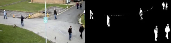
Motion detection aims to track the movement of an object or person. For example,

background subtraction (to be discussed further in section 1.3) can be used in a

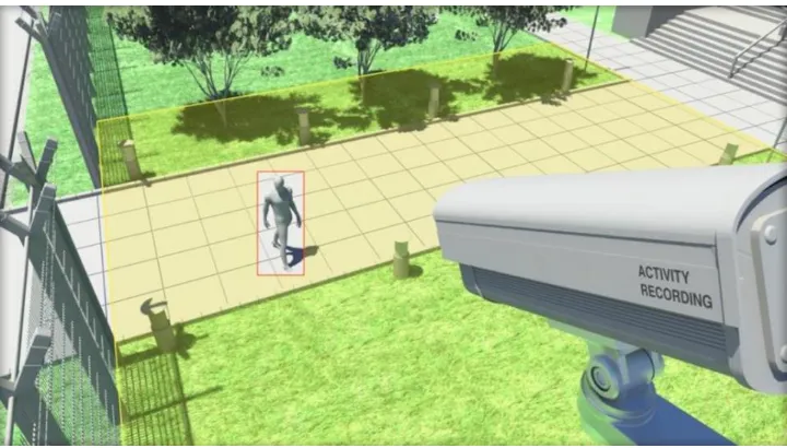
surveillance camera to monitor a specific area to automate motion detection, see Figure 1.

Motion detection is not limited to video surveillance, as it can be useful to track gestures,

posture and actions for possible applications in many areas, such as, Human-Computer

2

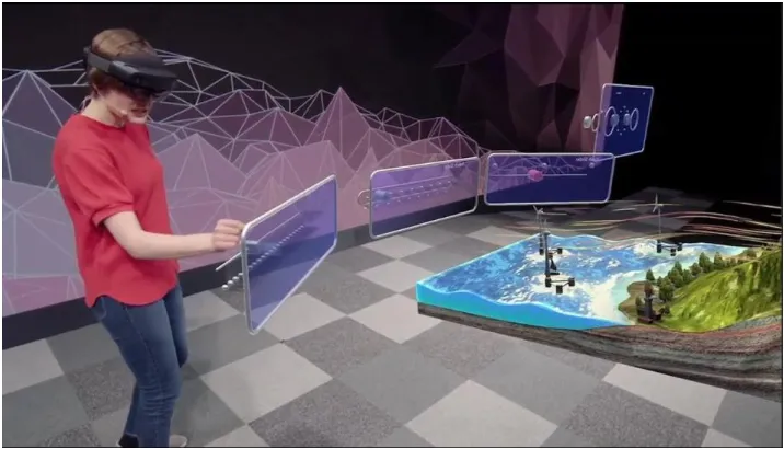
Many applications of motion detection can be incorporated into an augmented

reality device. Gesture recognition can be useful for device interaction to allow a user the

ability to react to a virtual scene and/or objects without the use of a controller, see Figure

2. Movement can be tracked for virtual object placement and occlusion. For example, a

person might walk in front of a virtual object and occlude part of the view of said object,

thus requiring the ability to understand a 3D environment.

Figure 1. A surveillance camera monitoring a path and detecting a person’s activity. (Image acquired from https://www.ips- analytics.com/en/products/ips-videoanalytics-new/server-based/ips-motion-detection.html).

Placement of virtual objects in augmented reality requires the ability to recognize

and reconstruct the scene. Scene reconstruction requires information about the 3D space

of the scene, including depth. An RGB camera can be used to recognize the scene, but an

image does not have depth information. This is because the camera projects a 3D space

into a 2D space to acquire the image, thus losing depth information through the loss of

the third coordinate of each pixel. In computer vision, many solutions can be applied to

3

from many sequential images captured from a single camera, or more sensors can

contribute information, such as a second camera for stereo vision, or other sensors like

LIDAR and RADAR for depth coordinates from a time-of-flight (ToF) sensor. With

depth information, the scene can be reconstructed virtually using estimated 3D

coordinates of each pixel in order to project virtual objects into the scene.

Figure 2. An image from Microsoft’s HoloLens 2 live demonstration. The user is interacting with virtual objects viewed from the created holograms within the HoloLens headset. The cameras on the headset detect the user’s gestures and allows the user to adjust differently styled buttons and sliders (seen in the image) just by grabbing them in air. (Image acquired from

https://www.youtube.com/watch?v=uIHPPtPBgHk).

In the last of our examples of fields in computer vision, we have applications to

object recognition. The biological system uses object recognition for many tasks, such as

reading the individual characters in a sentence or entire words at one time, understanding

our environment from the objects that surround us, and immediately recognizing a person

from their face. With recent developments in deep learning, object recognition has greatly

4

We further explain deep learning in computer vision in section 1.2, background

subtraction in section 1.3, obstacle detection in section 1.4, and change detection in

section 1.5. We present the problem statement in section 1.6, possible applications in

section 1.7, and finally the thesis organization in section 1.8.

1.2 Deep Learning

Computer vision has progressed rapidly through the use of deep learning. Specifically,

we utilize deep learning models, such as the Convolutional Neural Network (CNN), to

process images. At a high level, CNNs are special neural networks that use shared

parameters in order to scan images. Computer vision also makes use of dimensionality

reduction models, such as the autoencoder structure. An autoencoder aims to reduce the

incredibly high dimensionality of an input image (for computer vision tasks) into a set of

features that can be decoded to reproduce the original input image.

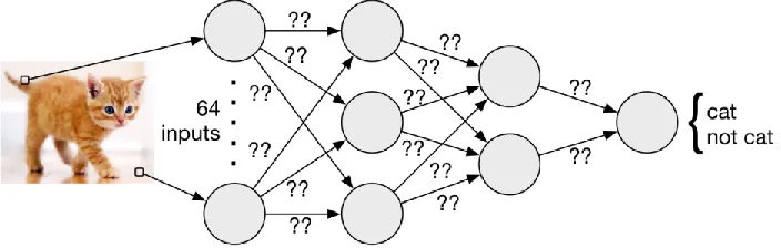
A neural network is a collection of nodes, called neurons, and weighted node

connections, see Figure 3. An input is flown through layers of neurons in order to

produce an output. In the case of computer vision, inputs can be images and the

associated outputs are labels for classification or ranges (continuous values) for

regression tasks. Each neuron is connected to several other neurons with an associated

weight to each connection. Inside the neuron is an activation function that transforms

inputs non-linearly. The neuron takes the dot product between the previous layer of

neurons and the connected weights as input. The output of the neuron is a non-linear

transformation of the dot product using the neuron’s activation function, such as ReLU,

Sigmoid, Tanh, and more. This is repeated for all the connected neurons through the

5

the problem in the case of classification or regression using functions, such as SoftMax,

Sigmoid, and more.

The neurons of a neural network can be viewed as feature detectors where a given

input is encoded into numeric values (features) as it is passed through the layers of the

network. Each layer would ideally (not always the case) learn progressively more

complex features of an input. The features are detected using a dot product to make a

comparison of the weighted connections and the outputs of the previous layer of neurons

(or the input itself). The neuron will output a value for the resulting comparison, which

represents a more complex and high level feature composed of the previously detected

features. At a high level, the network simply aims to learn its weighted parameters

through training of various input and output examples to detect valuable features of the

data. This then acts like a function relating the input examples to the output examples,

and can be, ideally, generalized to a larger set of related unseen inputs and outputs.

A loss function and gradient descent algorithm are used to tune the weights of the

neural network into producing the appropriate outputs. The loss function acts as a

mechanism to measure the difference between the currently poor output of the network

and expected (labelled/training) output of a given input. From there, the gradient descent

algorithm calculates gradients of each weight and the series of connected neurons through

back propagation based on the amount of loss described by the loss function. Gradient

descent describes the estimated direction to tune the weights while back propagation is

the process of tuning each weight as we backpropagate through the network

nodes/weights. As a result, each weight is slightly tuned for better results with each

6

Figure 3. An image of a cat is used as an input to 64 nodes, called neurons. These neurons feed into several layers of neurons (in the case of deep learning) until an output neuron is reached for a final classification of cat or not cat. Each neuron compares the connected weights to the output of the previous neuron (or an input value) through a dot product. Training data, a loss function and gradient descent are used to tune the weighted parameters of the network (the “??” over the connections) to properly classify the image as a cat. (Image acquired from https://homes.cs.washington.edu/~bornholt/post/nnsmt.html).

CNNs are neural networks designed to be more efficient for images. Images are

generally very large and costly to process. A neural network must have an input weight

for every pixel of an image. This is unrealistic in most cases, especially high resolution

images. To overcome this problem, CNNs use shared parameters to process and scan an

image. A neural network, called a filter in this case, processes a very small portion of the

image to produce a feature of the area. The filter is scanned using the same parameters

(hence the term shared parameters) over the entire image to produce a feature for each

region. There may be several filters processing the image and producing output, which

together create a set of feature maps as an output. This process of scanning is known as a

convolution. We can apply the convolution step to the produced feature maps of previous

layers with new filters. This allows the CNN to obtain the desired growth in feature

complexity the original neural network achieves by stacking layers of neurons. We may

also process feature maps with pooling and activation functions to further focus

7

non-linearly using an activation function. Once the feature map is small enough, we feed

the feature map entirely to a normal fully connected neural network to finally classify the

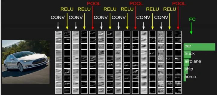
image. See Figure 4 for an example of a sequence of CNN steps. Training the CNN is

similar to training the neural network where we update the weights using a loss function

and gradient descent. The shared parameters of the filters are updated by accumulating

the gradient of contributing inputs processed by the shared parameter.

Figure 4. Here an image of a vehicle is processed by a convolutional neural network to recognize whether the image is a car, truck, airplane, ship or horse. Each column is a different step in the CNN process used (flowing from left to right). The boxes represent features produced in the current step of several filters. The first step is a convolution of shared parameters to generate a feature map. The next is the use of an activation function known as ReLU for non-linear processing. Occasionally pooling is used to focus processing on key information. Finally, a neural network is used to process the features and classify the image as a car. (Image acquired from http://cs231n.github.io/convolutional-networks/).

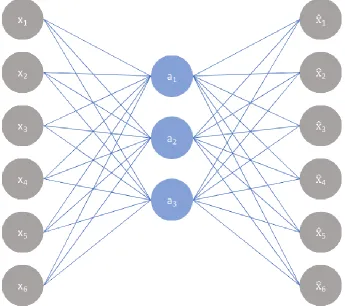
Finally, another important neural network is the autoencoder. The

autoencoder simply aims to compress an input into a feature representation,

known as dimensionality reduction. The network is built on two steps, an

encoding of the input and a decoding of features. The relationship of both

portions of the network can be seen in Figure 5. Previous networks discussed are

8

the opportunity to learn from labelled outputs, such as Cat or Not Cat. The

autoencoder is an unsupervised approach where there are no associated labels to

any input, because it simply learns the feature space of the inputs. The encoder

portion of the network is a simple neural network with features as outputs,

essentially skipping the final “output” layer with classification data. In order to

train the network, a decoder is used to reproduce the original image. The decoder

is just another neural network taking the features of the encoder as input and

producing the original image as output, though it is expanding into outputs rather

than shrinking into features. Together they make a large network. The images (or

samples) are used as both the input and the training “label” of the network. The

loss function compares the output image of the autoencoder to the original image

and describes the amount information lost between the images. Finally, gradient

descent adjusts the weighted connections to tune the network. The encoder and

decoder portions of the network can be split and used individually to compress

(encode) or decompress (decode) samples.

1.3 Background Subtraction

Background subtraction is a task where we aim to extract foreground information from a

sequence of images obtained through a stationary camera. Ideally, the images will have

each pixel labelled as black for background and white for foreground to visualize the

segmentation of the foreground, see Figure 6. This information can be used in a variety of

9

Figure 5. Example structure of an autoencoder with a single layer representing the features (neurons coloured in blue / placed in the center). The input is on the left, encoded into features in the middle and decoded into the original input on the right. The network can be detached to use the encoder and decoder individually. Many more layers can be incorporated into the autoencoder for a deeper network. (Image acquired from https://www.jeremyjordan.me/autoencoders/). (Best seen in colour).

Background subtraction has some areas of difficulty and limitations. The

sequence of images must be stationary. Often, this is not the case as camera jitter can be

present in the video feed, so methods must adapt to some movement. The background

may have some background noise or circular movement such as waves, grass/tree leaves

moving in the wind, and more. These motions should not be considered part of the

10

Figure 6. Example of extracting the foreground using a background subtraction technique, mixture of gaussian (MOG). (Images acquired from https://docs.opencv.org/3.4/d1/dc5/tutorial_background_subtraction.html).

Sometimes foreground movement may become part of the background, and other

times the background can become part of the foreground, due to some movement. For

example, a driving car is considered foreground, but when the car is parked it should

merge into the background. At the same time, a parked car can be part of the background,

but when the car is moved it should appear as the foreground. Another example would be

a floor mat which is considered part of the background. When someone comes around

and moves the mat in a different location, it should appear as foreground while being

moved, but merge with the background once stationary. There’s a related problem known

as ghosting where the initial location of a moved background object might remain as a

detected foreground, despite nothing being there. We are left with the “ghost” of the

object since the new background appears different from when the background object was

occupying that location. For example, in Figure 7 the mat that was moved will leave a

new background in its initial location, and could be detected as foreground since the new

floor is different from the mat. This would leave us with two mats detected, where one is

11

Figure 7. Example of the ghosting effect where a mat has been moved to another location leaving the ghost of the mat in its original position. (Image acquired from [12]).

Other difficulties can include lighting changes. For outdoor systems, light can

shift from day to night, clouds can cause sudden lighting changes, and shadows can move

with the sun. Lighting changes should be considered as part of the background and the

background model should adjust for dynamic changes through time. Additionally, sudden

bright areas, such as glares, can occur due to shinny surfaces and take up a large area of

the image. These glares should have no affect on the background or foreground objects.

Other lighting changes might be darker, such as shadows. Shadows caused by

background objects must be modeled over time if any movement occurs. Foreground

12

not want to include shadows in this case (though some algorithms include options to

detect shadows), thus the background model must be flexible in lighting conditions.

1.4 Obstacle Detection

Obstacle detection aims to detect obstructions of a path being travelled by an automated

vehicle (or to assist a person). For example, a robot travelling down a hallway might see

potential obstacles, such as people, walls, and other objects, along the path. The robot

does not have prior knowledge of the path’s floor or structure and must determine where

it is safe to travel. Obstacle detection relies on sensors to detect potential hazards, such as

one or more of the following: RGB camera, LIDAR, RADAR, ultrasonic, and more. For

example, a simple robot travelling a path might just need a single RGB camera, but a

self-driving vehicle might require several RGB cameras and depth sensors such as

RADAR and/or LIDAR (see Figure 8).

Obstacle detection has some areas of difficulty depending on the sensors used.

LIDAR might detect depth and overall 3D structure with high precision, but is expensive

and has low resolution. RADAR is generally less precise and slower than LIDAR, but

can penetrate through weather such as rain and snow. RGB cameras are affected by

lighting conditions, but are generally fast, precise, have high resolution, and are

inexpensive. In that case, our focus will be on the use of a single RGB camera, known as

monocular vision.

The main difficulty of monocular vision in obstacle detection is modelling the

floor and pixel depth. Monocular vision in obstacle detection relies on detecting obstacles

that appear different from the ground. Though depth can be estimated through a series a

13

appearance can lead to difficulties, such as sudden glares due to a shiny surface or a

sudden change in floor textures and patterns. Other difficulties can include obstacles that

appear similar to the floor creating false negatives.

Figure 8. Tesla’s autonomous vehicle sensors. Not shown are side facing and rear facing cameras. Sensor FOV is shown in this image and how each vehicle is detected using 8 cameras, RADAR and 12 ultrasonic sensors. (Image best seen in colour). (Image acquired from https://medium.com/self-driving-cars/tesla-enhanced-autopilot-overview-l2-self-driving-hw2-54f09fed11f1).

1.5 Change Detection

While obstacle detection aims at detecting obstructions and hazards to a path being

travelled, change detection while travelling a path only considers a change in the path.

Obstacle detection considers everything, apart from the ground, as a hazard or a

detectable object. The main difference between change detection and obstacle detection is

the background that is being modelled. Monocular vision obstacle detection methods

14

change detection in a path) would ideally model everything that is part of the path, such

as walls and other stationary objects.

Change detection aims at detecting a difference from prior knowledge. For

example, change detection in the form of background subtraction would extract the

foreground based on prior knowledge of the background (such as a video feed of the

area), so that the segmentation only contains relevant information. In a similar way,

applying change detection to obstacle detection would result in the detection of

obstructions that differ from prior knowledge of the path. For example, the walls would

be considered known and not a detectable change. At the same time, something missing

from prior knowledge can be considered as a detectable change (such as a missing wall),

but this might not be important for methods, such as background subtraction due to

problems like ghosting.

1.6 Problem Statement

We aim to implement change detection in a travelled path using monocular vision. We

are provided with a training video of the scene to be travelled. This video is ideally

obstacle free and any objects included in the video are considered part of the path. The

training video will show the path travelled in full. The robot that will be travelling the

path is assumed to know the path it must travel and the directions it must take. When the

robot travels the path during the test phase, it can utilize this training data to determine

any changes along the path, such as unseen obstacles. The detectable obstacles of a path

do not include elements such as walls and other objects within the training video. If a

detection occurs, the robot will simply halt, and either wait for further instructions or wait

15

1.7 Applications

This problem can be applied for robots travelling known paths, such as factory robots

with repetitive tasks with a need to detect possible obstructions and changes in their path.

This would allow for informed decisions about stopping or obstacle avoidance and other

operations available. This problem can also be applied to automated robots, such as home

cleaning robots where the environment is known. These robots can scan the environment

to learn the path which can be used as the training video. This would allow for detection

of new obstacles or movement of furniture to adapt to the environment. This could

provide an advantageous cost reduction and easy environment training with just a single

camera for detection.

1.8 Organization

This thesis is organized as follows: Chapter 2 reviews literature in background

subtraction and obstacle detection. Chapter 3 will go over a geometry-based approach to

solve the problem described in section 1.6. Chapter 4 will go over a second approach to

solve the problem with the use of deep learning using an ensemble technique. Finally,

chapter 5 will go over experimentation with results, and the thesis will be concluded in

16 CHAPTER 2

Previous Works

This chapter reviews literature related to change detection. We review work focused in

two main areas: background subtraction and obstacle detection. For background

subtraction in section 2.1, we focus on modelling background scenes using a stationary

camera. Section 2.1.1 reviews geometry-based techniques, while section 2.1.2 reviews

use of machine learning and deep learning techniques in background subtraction. We

continue with obstacle detection in section 2.2 where we focus on monocular vision

based obstacle detection methods. Finally, in section 2.3, we describe the relationship

between our work and both background subtraction and obstacle detection.

2.1 Background Subtraction

2.1.1 Geometry-Based Approaches

Oliver et al. [1] perform segmentation using an eigen space of the scene. The eigen space

is computed using several frames from history to build a mean-image and a covariance

matrix. They decompose the covariance matrix using an eigenvalue decomposition.

Finally, they use Principal Component Analysis (PCA) to reduce the space, and the

eigenspace model is created using the eigen vectors. This method is beneficial for moving

objects which do not appear in the same area for long. The model is unlikely to keep the

moving object in the model after using PCA, and it allows for segmentation of the

background.

Stauffer and Grimson [2] proposed the Gaussian mixture model (GMM) method.

17

different events to be modelled when the pixel no longer views the same location in the

real world due to jitter or background movement. The pixels belonging to the background

will gain weight while lowering variance as more data is assigned to the associated

distributions. Thus, any model the foreground produces will have a very low weight and

high variance compared to the background models. Overtime, if the foreground remains

in place, the data will accumulate in the foreground models by gaining more weight and

lowering variance, while the background models lose weight from lack of data through a

decaying process. In this case, the foreground will become the background which reduces

ghosting. The method requires a history to build the gaussian distributions. Authors in [3]

and [4] automate the number of components selected for the set of GMMs for each pixel

through a derivation from the maximum likelihood of the multinomial distribution (a

generalization of the GMM). Chen et al. [5] build on the GMM method by first using

image segmentation and merging regions of consecutive frames. Gaussian Mixture

Models are then used to model these regions, and foreground extraction is then

performed.

Wang et al. [6] create the method Flux Tensor with Split Gaussian models

(FTSG). They combine two techniques for background subtraction using K GMMs and a

Flux Tensor approach [7], [8]. Flux tensor is a motion detection technique which is

resistant to "complex scenes, lighting conditions and environmental variables" [7], but it

requires infrared technology, which is not our focus. This paired with GMM allows them

to "handle challenges such as shadows, illumination changes, dynamic background,

18

enhances this method in combination with other sensors, showing the importance of

advancing monocular vision techniques.

In [9], [10], authors implement the sigma-delta method. First, they calculate the

median of each pixel based on the given history of input images. Then, the difference is

taken between the current frame and the median image to calculate a motion likelihood

measure. The variance is computed in a similar way to the median for a measure of the

temporal activity. Finally, each pixel is classified as background or foreground based on

whether the motion likelihood outweighs the temporal activity. This allows classification

of background pixels when there is a cyclic motion in the background such as grass or

waves. With background noise cycling at a consistent rate the model will account for that

motion in the variance and only classify this movement as foreground when the motion

likelihood outgrows the variance.

Mandellos et al. [11] use background subtraction to track vehicles over highways.

The method slowly builds a median image as the background model waiting for vehicles

to pass through the highway. The assumption is that the background will be present more

often than the vehicles over time. This allows the algorithm to isolate the background

from the vehicles to create the background model. They further compare the median

image to new frames and finetune the segmentation.

In [12], authors proposed the ViBe method. As they describe in their paper, “our

proposed technique stores, for each pixel, a set of values taken in the past at the same

location or in the neighborhood. It then compares this set to the current pixel value in

19

choosing randomly which values to substitute from the background model” [12]. The

method requires a history of each pixel in order to build the background model.

St-Charles et al. [13], [14] proposed the SuBSENSE method. The method aims to

automate parameter changes when considering different or dynamic scenes. They

consider the built background model, the current frame, the frame distance, and pixel

movement to automatically adjust parameters as needed.

Sedky at al. [15] propose the Spectral-360 approach. They model the background

using a physics based dichromatic reflection model. The model assumes physical

properties: "there is a single light source that can be a point source or an area source; the

illumination has a constant [Spectral Power Distribution (SPD)] across the scene and the

amount of illumination can vary across the scene" [15]. They use a history of 60 training

frames to calculate the Correlated Colour Temperature (CCT) and the Surface Spectral

Reflectance (SSR). They build their model and use the SSR and CCT to compare with

new frames using an adaptive threshold to achieve a segmentation.

Wang and Dudek [16] use a history of frames to build K short-term templates and

a long-term template in an extended version of the background subtraction algorithm

AMBER [17]. These templates are composed of pixel values of the history using a

background value and an efficacy counter. The templates are ordered by the efficacy. The

long-term template is always first, as they place the values of highest efficacy in that

template. To classify pixels, all are considered foreground until a pixel matches one of

20

proceed to update the templates. Ghosting is handled by updating the background model

with foreground pixels that have gone unchanged for a period of time.

Zeng et al. [18] propose an algorithm for background subtraction called

Background Subtraction with Real-Time Semantic Segmentation (RTSS). They run

SuBSENSE [14] as the background subtraction algorithm and ICNet [19] as the semantic

segmentation algorithm in parallel to perform background subtraction through a

combination of their segmentations. SuBSENSE provides non-parametric background

subtraction and they further merge ICNet's segmentation for enhanced results.

SuBSENSE uses various functions to achieve a parameter-free design, see Figure 9 for a

diagram of the approach. They ([18]) further incorporate ICNet's segmentation into the

raw segmentation portion of SuBSENSE, rather than relying entirely on the foreground

segmentation (see Figure 10). Combining these two segmentations allow for results

exceeding some deep learning approaches.

2.1.2 Machine Learning Approaches

Cheng and Gong [20] propose a generalization of batch learning 1-SVM to classify each

pixel as background or foreground. They focus on efficiency and use parallel programing

to achieve real time processing at over 80 FPS.

Gregorio and Giordano [21] use weightless neural networks (WNN) (see [22] for

original paper on the WNN method) for background subtraction. They use pixels to

represent network nodes to classify the background and foreground. They maintain a

history of pixels for better classification to account for lighting and other changes. [23]

uses weightless neural networks to track motion to allow a robot to follow a leader. The

21

Figure 9. The SuBSENSE approach described in [14]. An input frame is compared to the maintained background model. The background model is maintained through several functions dynamically updating thresholds for segmentation, distance and noise levels. Finally a foreground segmentation is produced and post processing is performed on the resulting segmentation. (Image acquired from [14]).

Figure 10. The proposed method in [18]. They alter the SuBSENSE approach in [14] (see also Figure 9) by using ICNet’s segmentation [19] of the image along with a foreground segmentation produced by the algorithm to refine results in post processing. (Image acquired from [18]).

Braham and Droogenbroeck [24] perform background subtraction in their

proposed method by using a Convolutional Neural Network (CNN). They use 150 frames

of a video sequence to obtain a grayscale temporal median. They train the network using

22

background subtraction algorithm. From there the CNN performs background subtraction

using the current and median frame. Babaee et al. [25] also perform background

subtraction using a CNN with additional post processing to smooth out the resulting

background subtraction. They trained their network using the output of SuBSENSE.

Ciocca and Schettini [26] use an ensemble approach to perform background

subtraction. They use several different background subtraction methods combined, using

a genetic algorithm. They show that a combination of some of the simpler algorithms can

perform better than any of the more complex algorithms they tested.

Sakkos et al. [27] use a convolutional network to perform background subtraction

without a background model. They use 10 frames as input, but the frames are not

concatenated as one input. They use four parallel convolution steps, each with 4 frames

as input from a sequence of 10 frames (see Figure 11). The CNN further merges the

convolution outputs. An upsampling of the output of the CNN at various steps are used to

produce a full resolution background subtraction. Their model is trained on all scenes in

the tested datasets, rather than each individual scene.

Authors in [28] use a convolutional autoencoder to produce a background

subtraction. The input is the foreground segmentation of three other methods:

SuBSENSE [14], FTSG [6], and CwisarDH+ [29] (based on weightless neural networks).

The segmentations of these algorithms are encoded in order to extract features of the

techniques (see Figure 12). The features are decoded into a segmentation of the

foreground and trained on the ground truth segmentation. They show their approach

23

Figure 11. Convolution steps of the background subtraction network proposed in [27]. A series of images are fed into the CNN in parallel allowing for a 3D convolution for background subtraction. Yellow represents upsampling of the segmented foreground with connected outputs from the CNN. (Image acquired from [27]). (Best seen in colour).

24

2.2 Obstacle Detection

Lorigo et al. [30] use a three component system for obstacle detection. Each system uses

a different method of detection through brightness, RGB, and HSV. They slide a window

over vertical strips of the image to detect obstacle boundaries. Detected edge segments

are combined to create a smooth boundary segmentation of the obstacle. Commands are

generated for their robot based on the boundaries imposed by the detected edges. They

tested this robot in different environments with the camera placed relatively close to the

ground.

Ulrich and Nourbakhsh [31] use a ROI to convert the entire frame into a

segmentation of the ground in black and possible obstacles in white. They use a

histogram of the hue and intensity of the HSI colour space within a ROI covering the

direct path of the robot. This models the ground and is then compared to the rest of the

frame for classification. Obstacles cannot be present in the ROI and the ROI must be

sufficiently large enough to model the ground. This method was tested using a robot in

both indoor and outdoor environments. Similarly, Raj et al. [32] also use a histogram of

the image to classify the image into ground and obstacle segmentations.

Michels et al. [33] performs obstacle detection in a forest a using remote

controlled vehicle. They train a linear regression model to estimate depth of trees using

both simulated and real data. They use windows scanned vertically along strips of the

image to estimate tree boundaries and obtain controls for the remote car to avoid

collision. The locations of trees are determined by their horizontal position in the image

25

Li and Birchfield [34] train anSVM model to classify vertical and horizontal lines

obtained through edge detection. This allows them to generate a segmentation through

connected vertical and horizontal lines to determine the wall-floor boundaries. This

provides the estimated safe region to navigate, though they do not directly attempt to

detect obstacles aside from the walls. The method has difficulty with textured floor

patterns, which creates confusion for wall boundaries due to the lines generated from the

textures.

Jia et al. [35] perform detection on roads. Obstacles are detected in the bottom

half of the image, up to the horizon of the roads tested. They use a two consecutive

frames (TCF) approach to analyze feature points and calculate their change between

frames. Then, they filter feature points that should be kept through a confidence measure

based on the calculated height and distance of each feature point. They show good results

in the KITTI dataset at detecting objects by differentiating obstacles from their shadows

and other lane markings to avoid false positives through a sense of height and depth.

Souhila and Karim [36] use optical flow in a sequence of images to detect

obstacles. Optical flow is the measure of 2D motion induced by a 3D motion in a 3D

scene. They calculate several vectors over consecutive frames which describe the

movement of pixels through their intensities, which in turn provides the 2D motion. They

estimate the Focus of Expansion (FOE) which is the point where the motion vectors are

directed away (or expanding from) in the 2D image plane, see Figure 13. They use the

information from optical flow to estimate the time to contact and depth information.

26

balance out the amount of flow on the left and right sides of its view. The method relies

on the flow of an obstacle to be greater than the flow of a safe region to travel.

Figure 13. Example FOE given many motion vectors (arrows). The left (L / Hl) and right (R / Hr) motion vectors are estimated and are pointed left and right, respectively, from the FOE. (Image acquired from [36]).

Similarly to [36], authors in [37] use a simple corner detector to obtain feature

points in order to reconstruct the scene from optical flow. They use this information to

detect obstacles ahead of a vehicle. While driving the car, other cars and motions greatly

affect the estimation of the estimated FOE using optical flow. Instead, they use straight

lines from the edges of the lane lines of the road where the intersection of the straight

lines are estimated to be the FOE, see Figure 14. Using this FOE, they estimate distance

information and reconstruct the scene which provides the obstacle information through

27

Figure 14. Parallel lane lines are interesting at a point infinitely far away due to camera projection. If we are travelling forward within the lane boundaries, we can expect the scene to expand (roughly) from this point. We can use this point as an estimate of the FOE. (Image acquired from [37]).

Authors in [38] use several images in a monocular camera to reconstruct the

scene. The method aims at detection approaching obstacles within a vehicle’s rear-view

camera. The method has three key steps: first they detect feature points in the series of

frames, then they reconstruct the scene, and finally classify points to detect obstacles.

They use feature points with constant motion on the ground region and discard feature

points with low quality disparity. These feature points are used to estimate vehicle

motion. From there, they reconstruct the scene using matched feature points and

triangulation equations for depth information. Triangulation is a process where we take a

point of an image, and its identical point in another image (another view of the same

scene), and calculate the depth and/or third coordinate of that scene point using

calibration information of the camera. Each feature point is then labelled as an obstacle or

part of the ground features. They use the height of the vehicle's camera as their threshold

for obstacle classification where feature points below 20% of the camera’s height are

considered part of the ground. Finally, they report the nearest obstacle back to the driver.

Zhou and Li [39] assume that the ground plane will have the largest number of

feature points. This assumption allows them to estimate the ground plane from the ground

28

which mostly stabilizes the camera movement, thus creating a smooth movement in

ground features. Then, they calculate a normalized homography of the ground plane

using RANSAC. A homography is a matrix which describes the transformation between

two views of a scene. In this case, they use a sequence of images from a monocular

camera and estimate the ground plane with the homography. RANSAC allows them to

search for the dominant plane (of the many possible ground planes) given the outlier

obstacle points. A homography can be calculated using 4 points from each plane. As

mentioned before, potential obstacles may cause error in the calculations of the

homography. Thus, choosing any 4 points can result in a bad homography and a bad

estimation of the ground plane. RANSAC searches for the best set of points (or a local

minimum) to calculate the best estimate of the homography. Given many points of the

ground plane (including obstacles), RANSAC searches for 4 points that result in a

homography plane closest to all points, allowing for error and removal of outliers. The

dominant ground plane is likely to be chosen, if it contains a significantly large amount of

feature points, and the ground can be determined. Once the ground plane is determined,

the feature points can be classified as part of the ground plane or part of an obstacle based

on their distance from the plane.

Conrad and DeSouza [40] modify the Expectation Maximization (EM) algorithm

with the ground plane homography in order to cluster feature points as part of the ground

plane or part of an obstacle. EM is an unsupervised clustering machine learning

algorithm. This means that there are no associated labels to any data point. The EM

algorithm simply aims to find a relationship in the data through a grouping known as

29

a two-step iterative process. EM depends on an initial guess of the samples and cluster

distributions, then iterates in a two-step process. In the first step, the algorithm proceeds

to fit a number of distributions to the labelled data, depending on the number of

predefined clusters. In the second step, the samples are assigned to the nearest

distribution and relabeled. This process will iterate until the distributions stabilize

between the two steps. Finally, the algorithm is left with several clusters of similar

samples. In the case of detecting obstacles, they cluster feature points with a modified

EM algorithm. The algorithm is designed to cluster the data based on the ground plane

homography between two images. Feature points that are part of the ground plane are

grouped, while other points are grouped as obstacle points. See Figure 15 for an example

of the resulting classification of feature points.

Kumar et al. [41] first calculate point correspondences between two frames using

feature points. Then, they calculate the ground plane homography using optical flow and

classify features as part of the ground plane, part of an obstacle, or ambiguous. Image

segmentation is performed on the image and they further classify entire regions of the

segmentation as an obstacle or part of the ground plane. The segmented regions are

classified by the majority of labelled points in that region.

Kumar et al. [42] use ground plane homographies using two images and detect

superpixels on the image to cluster similarly neighbouring pixels together forming

"superpixels." They perform edge detection and filter lines that are not vertical. They

further warp the image into a different perspective to filter out lines that are not part of

the obstacles, since it is expected that floor lines will not deviate nearly as much as

30

finally classify each pixel as the floor or an obstacle. The Markov Random field is used

as an undirected probabilistic graph where the superpixels are nodes, the edges (that were

previously detected in the image) are the edges connecting the superpixel nodes, and the

cost function is the resulting segmentation. The resulting segmentation outlines obstacles

from ground plane.

Figure 15. Feature points classified as ground plane (black) or part of an obstacle (light blue). (Image acquired from [40]). (Best seen in colour).

Lee et al. [43] improve on the proposed method in [42] and use an improved

Inverse Perspective Mapping (IPM) approach that is beneficial to camera placements that

31

and a ROI is used to classify each pixel as the floor or an obstacle. The system relies on

the number of edges, so if at any point the number of edges become inconsistent, they

further process the image to detect obstacles. They test a robot vacuum indoors in the

same indoor scene for a total precision, false positive rate, and recall of 81.4%, 5.9%, and

74.4%, respectively. Their results improve on [42], which achieved (in the same data) a

total precision, false positive rate, and recall of 57.4%, 14.2%, and 37.6%, respectively.

However, they needed to modify the algorithm in [42] to fit low camera placements.

Xie et al. [44] use reinforcement learning to train a robot obstacle avoidance.

They use two connected architectures to perform depth estimation and produce Q-values

in the reinforcement learning Q-network. The Q-values provide information on the

actions of the robot, such as linear action and angular action. The input to the

reinforcement model is the output of a depth estimating CNN. This CNN takes an RGB

image as input and produces a depth map of the scene as output. See Figure 16 for the

overall structure of the model. Training takes place in a simulator and testing takes place

in the real world, however, they needed to add noise, by blurring part of the simulated

input images, for better results in the real world. They test the robot in a few scenes and

show some examples of the robot circling around a room filled with randomly placed

obstacles. Similarly, authors in [45] use 4 consecutive depth maps and a CNN trained

through reinforcement learning. The CNN has two convolution steps and is finally fed

into a fully connected neural network. The resulting outputs are 8 Q-values where 3 are

actions for linear velocity and 5 are actions for angular velocity. The network is trained in

simulation, though the depth maps are acquired through a depth sensor rather than a

32

Authors in [46] use a horizon line of the image to detect obstacles for small flying

vehicles that know their altitude. The idea is that the horizon line will intersect obstacles

at the same height of the robot which will provide an uncertainty level applied to the

obstacle above and below the horizon line. Note that this means obstacles completely

below or above the horizon line will not be considered as obstacles. The ground and sky

are less likely to intersect the horizon line and a higher certainty is labelled to those

pixels. The uncertain pixels are classified as obstacle points and the certain pixels as

non-obstacle points using a random forest classifier. See Figure 17 for an example

segmentation of obstacles in the KITTI dataset.

Figure 16. This is the architecture of the convolutional neural network described in [44]. They use a depth prediction CNN and a Q-network to produce actions based on the resulting depth. The network is trained through reinforcement in a simulation. (Image acquired from [44]).

Xue et al. [47] detect obstacles at a far distance, see Figure 18. They use a

combination of an occlusion edge map and a regressor. The occlusion edge map is

generated by using a far-to-near approach to estimate edges at different distances in the

image/scene, with a fusion of edges in a near-to-far approach of the same image. This

allows detection of edges around obstacles at many different distances in the scene.

Finally, superpixeling is performed to completely fit edges around the small obstacles at

different distance levels. They use random forest to generate a high regression value for

33

Objectness Score (calculated likelihood a box contains an obstacle), and (4) Colour.

Using these features they are able to predict obstacles at various distances in an image.

Figure 17. Example obstacle segmentation in the KITTI dataset using the horizon line approach described in [46]. They provide an example for each row. From left to right, columns show: an input RGB image, a classification of the horizon, an uncertainty map of potential obstacles that intersect the horizon line (red is obstacle, blue is non-obstacle) and finally an obstacle map where white is obstacle and black is non-obstacle. (Image acquired from [46]). (Best seen in colour).

34

2.3 Relation to our Work in Change Detection

Our work in change detection uses components from both background subtraction and

obstacle detection fields. At the same time, our work is not completely part of either field.

In this section, we will go over the differences and relationships of our work to both

background subtraction and obstacle detection.

First, background subtraction methods aim to model the background of a scene

using a stationary camera. We also aim to model the background of the scene (of the path

we are travelling), though the camera is not stationary. This is a key difference in both

approaches since background subtraction techniques have the opportunity to use

hundreds of frames of the same portion of the scene and have a large description of the

dynamic changes of each pixel, such as lighting and background motions. Our work uses

a single video of the current path travelled resulting in just a few frames of information

for a given portion of the scene.

Finally, monocular vision obstacle detection methods do not use a training video

of the path. Using a video of the scene allows us to differentiate, with a much higher

confidence, important changes from general obstacles that are part of scene. This is an

advantage in robots that travel known paths multiple times to perform a task. The robot is

assumed to know where it is travelling and we simply aim to detect sudden changes in the

path, which could harm either the robot or the person and/or object in the robot’s direct

path. Another key benefit to the use of a training video is the ability to determine the

robot’s current location within the path. We can match the robot’s current view of the

35

Positioning System (GPS) and allow positioning in environments lacking a GPS signal,

36 CHAPTER 3

Geometry-Based Methodology

In this chapter we present our methodology for the geometry-based approach with the use

of vision techniques. In section 3.1, we explain the motivation of the method with a slight

overview of the approach. In section 3.2, we explain the details of the methodology of the

geometry-based approach.

3.1 Motivation

In this approach, we use geometry-based techniques to detect changes along a path. The

method is split into two main steps. First, we analyze a set of test frames in order to

determine our current location within the training video. This provides us with a

neighbourhood within the training video of possible matching training frames to the

given test frame. The second step is to have the robot proceed and start detecting

obstacles. Changes are detected through a comparison of the current testing frame and the

best matching training frame. The search for the best matching training frame is found

within a few seconds of the current location within the training video. See Figure 19

where we provide a visual for the setup of the comparison between both matching

frames. The comparison uses histograms of a ROI to detect a change in the variance of

the colours in both frames. The robot may halt if a detection occurs. Otherwise, we

proceed with the next test frame and shift the neighbourhood to center around the

37

Figure 19. We visualize how two frames are set up for comparison. The test frame with changes (on the right) is registered onto the best matching training frame (on the left). This aligns the scenes in both frames. Then the ROI can be placed in the same area of both frames overlooking the same portion of the scene. (Best seen in colour).

3.2 Geometry-Based Approach

A high level pseudocode is presented in Algorithm 1. The algorithm only presents two

procedures, one to determine the current location, as seen in section 3.2.1, and the other is

the overall change detection approach, once a location is determined. The algorithm runs

the first procedure only one time, then the second afterwards. We discuss first how the

location is found in section 3.2.1 and how we match frames in section 3.2.2. From there,

we explain how we compare matching frames through frame registration in section 3.2.3.

38

3.2.1 Determining Current Location

Initially, the robot must determine its current location within the given training video,

essentially positioning itself within the path. The robot may be halted during this process

since we have no information on possible path obstructions. Once a location is

determined, we can start change detection from the first frame. The process of

determining the initial position of the robot is a one-time step and does not need to be

performed once detection starts. The location will be updated as the robot travels through

the path.

In order for the robot to position itself, we consider a set of N initial testing

frames. In our experiments, 2 frames were enough to determine a reliable location.

Choosing N greater than 2 allows for more confidence in the current location for dynamic

and moving background elements. For each of the N frames, we perform a grid search

along the entire training video to find their respective best matching training frame. We

define the best matching frame as the most similarly positioned training frame through a

compromise between real world location and camera angle. Neither of these metrics are

available to us directly, so we perform frame matching through feature point registration

which is further explained in section 3.2.2. Finally, once all frames have their respective

matches, we consider the median position within the training video. This is the most

frequently occurring position and is the probable area of the training video within the

39

Once a location is determined, this allows us to significantly reduce the search

space to a very small neighbourhood of the training video centered on the determined