Abstract
SWAIN, JEFFREY BRANDON.The Effect of Spatial Resolution on an Object-Oriented Classification of Downed Timber. (Under the direction of Heather Cheshire).
Advancements in remote sensing technology continue to aid natural disaster
damage assessment. Quick and accurate damage assessment significantly increases the
speed of recovery efforts and allows aid to reach those most severely affected.
Object-oriented classification techniques require minimal user input to remotely classify large
areas and may be utilized to provide timely and accurate damage assessments of affected
areas. In this study, I explored the use of object-oriented classification techniques to
classify downed timber areas in the Dare County Bombing Range in North Carolina. The
spatial resolution of scanned color-infrared aerial photography was degraded from
0.2-meter to 3 other spatial resolutions (1-0.2-meter, 5-0.2-meter, and 10-0.2-meter). Training data
developed from the 0.2-meter pixel imagery were used to establish training data for all
spatial resolutions. Each set of images was classified using object-oriented classification
techniques. Results were compared statistically to each other and to results obtained
from a manual delineation and a conventional supervised classification. Before the
accuracy assessment began, we anticipated that the classification produced by the
0.2-meter imagery would be the most accurate due to the high level of detail in the imagery.
After comparing the results of the classifications, there was no statistically significant
difference among the object-oriented classifications, but there was a significant
difference between the object-oriented results and the other classifications. Using the
training data created on the high-resolution imagery to classify the coarser spatial
resolution imagery did not cause classification accuracy loss. The potential damage
assessment impact of this technique is that low-resolution imagery can be utilized to
quickly classify damaged areas, provided high-resolution imagery is used to create
training data. This classification technique demonstrates that damage assessment can be
THE EFFECT OF SPATIAL RESOLUTION ON AN OBJECT-ORIENTED CLASSIFICATION OF DOWNED TIMBER
by JEFF SWAIN
A thesis submitted to the Graduate Faculty of North Carolina State University
in partial fulfillment of the requirements for the Degree of
Master of Science
FORESTRY
Raleigh, North Carolina
2007
APPROVED BY:
_________________________ _________________________
DR. GEORGE HESS DR. STACY NELSON
Dedication
I would like to dedicate this to my wife, Laddie, who has put up with continual
promises to have this research done and has stood by me through thick and thin. I would
also like to thank my parents, without their support and guidance none of this would have
Biography
The author is originally from Milford Delaware and moved to North Carolina in
1993. He has an undergraduate degree in Environmental Studies from Elon University
where he graduated with honors in 1997. He served in the North Carolina National
Guard from 2000 to 2006 and was activated as part of Operation Noble Eagle in 2003.
Acknowledgements
I would like to thank my committee members, Dr. Heather Cheshire, Dr. Stacy
Nelson and Dr. George Hess. I would also like to thank Justin Shedd, Jennifer Miller,
Table of Contents
LIST OF TABLES………..…. LIST OF FIGURES………... 1. BACKGROUND………..… 2. LITERATURE REVIEW………..…..
2.1 Hurricane damage to forest stands………..…. 2.2 Advancements in remote sensing applications
for hurricane damage……….…. 2.3 Current natural disaster remotely sensed
damage assessment techniques………... 2.4 Advantages of object-oriented classification
over pixel-based classification………..…. 2.5 Similar study………..… 3. OBJECTIVES ………...
3.1 Purpose………..…… 3.2 Hypothesis………... 4. METHODS AND MATERIALS………. 4.1 Study area………..…… 4.2 Imagery………..……. 4.3 Training Procedure……….…….. 4.4 Classification……….……. 4.4.1 Object-oriented……… 4.4.2 Supervised………... 4.4.3 Manual……….. 4.5 Accuracy Assessment……….. 5. RESULTS……… 5.1 Accuracy………. 5.2 Maps……… 5.3 Area comparison………... 6. DISCUSSION OF RESULTS……… 7. LIST OF REFERENCES………... 8. APPENDIX………..
8.1 Discussion of Imagery……….. 8.2 Discussion of Software………. 8.3 Solutions………. 8.4 Recommendations……… 8.4.1 Image Specific……… 8.4.2 Feature Analyst Specific………..
List of Tables
TABLE 1 Number of training polygons by class used for
List of Figures
FIGURE 1 Study area location………... FIGURE 2 Bullseye input representation……….……. FIGURE 3 Kappa z statistic computation………... FIGURE 4 Z statistic test computation………..…….... FIGURE 5 Comparison of accuracy assessment results………...…… FIGURE 6 Original 0.2-meter image and classification………..….... FIGURE 7 1-meter image and classification………..…... FIGURE 8 Original image and manual classification……….….... FIGURE 9 Total downed timber area comparison……….…... FIGURE 10 Setup learning options for Feature Analyst………... FIGURE 11 Input representation for 1-meter, 5-meter and
10-meter classifications………..…… FIGURE 12 Input representations for 0.2-meter classification……….... FIGURE 13 Learning settings in Feature Analyst………..… FIGURE 14 Original 0.2-meter image and classification mid-view………….……….... FIGURE 15 Original 0.2-meter image and classification far-view………... FIGURE 16 1-meter image and classification far-view……….… FIGURE 17 5-meter image and classification mid-view………... FIGURE 18 5-meter image and classification far-view………..…... FIGURE 19 10-meter image and classification close-view……….. FIGURE 20 10-meter image and classification mid-view………..…... FIGURE 21 10-meter image and classification far-view……….….. FIGURE 22 0.2-meter image and manual classification
far-view……….………...…. 10 14 19 19 21 22 23 25 26 41 41 42 42 43 44 45 46 47 48 49 50 51 52 FIGURE 23 0.2-meter image and manual classification
1. Background:
Natural disasters have occurred throughout modern history and have varied in
frequency and severity. Relief and recovery efforts have also changed to meet new
challenges. There are many factors that hinder relief efforts especially concerns about
where to allocate resources, how much is needed where, and who is affected most. All of
these decisions are based on best available information. The manner in which disaster
recovery information is collected has changed in many ways. Eyewitness reports and
ground surveys are giving way to modern remote sensing techniques using aerial imagery
and advanced image interpretation technology.
While there are a many factors propelling improvements in remote sensing
technology, disaster recovery applications have received added attention in the wake of
Hurricanes Katrina and Rita and the Sumatra-Andaman earthquake. As the severity and
graphic extent of a disaster increases, so does the value of remote sensing to aid recovery
efforts. Remote sensing technology was used to identify damaged areas and facilitate the
allocation of resources in the Sumatra-Andaman earthquake. Comparing before and after
images of the coastline guided the rebuilding of the coastline and the coordination of
activities among government organizations (Polngam 2005). Commercial and military
imagery was utilized to help The Federal Emergency Management Agency coordinate
relief efforts for Hurricanes Katrina and Rita (Adams 2005). In these cases, remote
sensing technology and satellite imagery assisted relief efforts through visual inspection.
In my research, I will validate the use of object-oriented classification as a remote
Technological advances in aerial and space-borne imagery have improved the
quality and availability of information. Imagery is now available through many
commercial entities at many different spatial resolutions. Satellite imagery is available
from many different sensors, such as, IKONOS, Quickbird and SPOT. Airborne sensors
from aircraft can provide imagery at even finer spatial resolutions.
Improvements in classification technology have also increased the quality of
information that can be acquired through remote sensing. Pixel-based and
object-oriented classification techniques harvest useful data for planners and scientists from
satellite imagery. Pixel-based classification techniques are used to classify coarse spatial
resolutions, like Landsat imagery (Blaschke and Strobl 2001). Pixel-based classification
ignores any spatial characteristics and focuses purely on spectral qualities.
Object-oriented classification examines the spatial relationship of pixels as well as spectral
qualities. This technique is designed to classify images with a finer spatial resolution
(Jensen 2005). The “objects” identified consist of similar pixels that are in close
proximity, producing a series of numerous polygons. The primary advantage that
object-oriented classification has over pixel-based classification is that the pixels are not
classified in isolation but in context with the rest of the image.
Object-oriented classification can be achieved through segmentation or user
specified algorithms. Segmentation divides an image into areas of like pixels and users
define the class of each group of pixels. The ‘user specified’ algorithm requires the user
to define areas on an image before classification can begin. Once the training datasets are
defined, the software uses the input to define the image. Visual Learning System Inc.’s
comparison techniques to classify images. Feature Analyst uses a supervised
classification method in which the program “learns” what each class is according to user
input. With well-developed training data, the software package can correctly recognize
and classify pixels faster and more thoroughly than manual classification, which can
greatly aid recovery and restoration efforts in areas devastated by natural disasters, such
as hurricanes. Object-oriented classification may be the best way to access more useful
and timely information for disaster recovery efforts.
2. Literature Review
2.1 Hurricane Damage to Forest Stands
Hurricanes are tropical cyclones that can produce extremely high winds,
tornadoes, torrential rain, and drive storm surge onto coastal areas (Anonymous 2007).
Large-scale canopy disturbances caused by windstorms or other catastrophic events affect
many forests (Merrens and Peart 1992). The two major types of damage to forest stands
caused by hurricanes are defoliation and flooding. While defoliation is the most common
type of damage, branch loss and uprooting of stems also occur (Brokaw and Walker
1991). Windfalls caused by hurricanes consist mostly of uprooted trees (Berg 2004), but
stand gaps caused by wind can have an irregular shape with many trees still standing
within each gap (Greenburg and McNab 1997). According to Berg, “hurricanes create
unique understory plant microsites and massive amounts of tree debris,” which “vary
substantially from man made gaps” (Berg and Van Lear 2004).
2.2 Advancements in Remote Sensing Applications for Hurricane Damage
Service has used Geographic Information Systems (GIS) to manage resources and aid in
land management planning (Parsons and Orleman 2002). To fully understandthe scope
and magnitude of storm events, “quick and reliable information on the extent of forest
damage is required.” (Scwarz et al. 2003). According to Adams (2005), recent
deployments of remote sensing technology have yielded many benefits including
“detailed visualization, regionwideassessment, safe surveying of dangerous areas, timely
information about inaccessible locations, and a permanent record of perishable damage.”
Rejaie and Shinozuka (2003) believe that recent advancements in remote sensing
technology have made it possible to remotely assess areas damaged by natural disasters.
Rapid deliveries of remote sensing products and on-site GIS have become invaluable
tools that increase the accuracy and timeliness of results (Parsons and Orlemann 2002).
2.3 Current Natural Disaster Remotely Sensed Damage Assessment Techniques
Remotely sensed data are being used more frequently to classify and assess
damaged areas all over the world. One of the most widely used remote sensing
techniques is change detection, which determines damage through a temporal analysis of
a location; areas that have changed are considered damaged. New techniques that utilize
user input to develop algorithms that classify damaged areas directly from one set of
imagery are becoming more prevalent.
Change detection has been the most widely used remote sensing technique to
assess damaged areas, but there are other techniques, such as principle component
analysis, maximum likelihood and complex coherence analysis. Rejaie and Shinozoka
1995 Kobe earthquake to determine damage. They attempted to classify each image into
changed and unchanged classes but were limited in application to places where
illumination conditions were identical. Kaya et al. used change detection to determine
damaged forest areas in Instanbul, India (1998). Thirty-meter pixel Landsat 5 Thematic
Mapper (TM) imagery taken in 1984 and 1997 were classified with a maximum
likelihood classification algorithm and compared visually to demonstrate the growth of
the mining industry at the expense of forested areas in India. Yamazaki compared the
backscattering characteristics of Landsat TM imagery in a complex coherence analysis to
synthetic aperture radar in Kobe, Japan to detect damaged buildings (2001).
Object-oriented classification techniques have also been used to classify damaged
areas. Redmond and Winne (2001) used Feature Analyst to classify two, thirty-meter
pixel Landsat 7 images according to burn severity. The thematic maps produced were far
more accurate than those created using principal component analysis (Redmond and
Winne 2001). Feature Analyst was also used to update fire load datasets in the
Petersburg National Battlefield and Shenandoah National Park (Shedd et al. 2005). To
classify downed woody debris, they used one-half meter true color and color infrared
aerial photography. Feature Analyst was successfully used to classify woody debris and
update the fuel load datasets in an accurate and time efficient manner.
2.4 Advantages of Object-Oriented Classification over Pixel-Based Classification
By incorporating both spectral and spatial image information, object-oriented
classification interprets information as the human eye does, yet has the advantage of
on objects, or “homogeneous groups of pixels” that relate to items of interest (Blaschke et
al. 2000). Single pixels are not as critical to understanding an image’s information as
objects and their relationships are (Blaschke et al. 2000). By incorporating user input,
object-oriented classification takes advantage of the user’s insight to identify image
objects (Blaschke et al. 2000).
2.5 Similar Studies
My study was built upon the results of three similar studies. Benson and
Mackenzie (1995) examined the effects of spatial resolution on remotely classified maps
of the Wisconsin Lake District. The objective of their study was to examine how
different spatial resolutions affected the classification of land cover on satellite imagery.
They used three different sensors: 20-meter SPOT multi-spectral, 30-meter Landsat 4 and
5 TM, and 1.1 kilometers Advanced Very High Resolution Radiometer (AVHRR). Each
image was classified with Leica Geosystems Erdas Imagine into two classes; water and
land. Classification values from these three thematic maps were used to extrapolate
several landscape parameters including percent water, number of patches, and average
area of patches. The extrapolation algorithm simulated classifications starting at 20
meters and then degraded by a factor of two until a spatial resolution of 1280 meters was
reached. Benson and Mackenzie (2005) found that as spatial resolution was degraded,
the number of water bodies identified, the percentage of total water and average patch
size decreased.
Scwarz et al. (2003) evaluated different classification algorithms on images with
IV, and 1-meter IKONOS. Object-oriented and supervised pixel-based classification
algorithms were used on each image and compared to a hand-delineated thematic map.
Scwarz et al. (2003) used image segmentation by Defines’ eCognition software and
compared it to a supervised pixel-based classification method. After all the images had
been classified, the accuracy was assessed and a Kappa statistic was generated. They
found that manual classification of the 1-meter IKONOS imagery was the most accurate,
followed by the object-oriented classifications of the IKONOS and SPOT images. The
most accurate pixel-based classification was the 10-meter SPOT IV image. Although the
object-oriented classification was not the most accurate classification, it was more
accurate than traditional pixel-based supervised classification at different spatial
resolutions.
Shedd et al. (2005) used Feature Analyst to classify downed woody debris on
0.5-meter aerial photography of Petersburg National Battlefield and Shenandoah National
Park. My decision to use Feature Analyst as the object-oriented classification software
was based on the success that Shedd et al. (2005) had using it. A true color 1:6000 photo
mosaic with a one-half meter spatial resolution was used for classification. Shedd et al.
(2005) were able to successfully classify individual downed timbers through multiple
classification runs. The ‘downed timber’ polygons were then used to augment fuel load
3. Objectives
3.1 Purpose:
In this study, I used infrared aerial photography to identify and classify areas of
downed timber. I compared an object-oriented classification approach with results
obtained from hand-delineation and supervised classification. The study area was part of
the Dare County Bombing range, which has been affected by Hurricanes Dennis (1999),
Floyd (1999), and Isabel (2003), creating large sections of downed timber. Three spatial
resolutions derived from the original aerial photography were chosen to simulate several
satellite sensors. The original imagery had a spatial resolution of 0.2-meters and was
degraded to 1-meter (IKONOS), 5-meter (SPOT IV Panchromatic), and 10-meter (SPOT
V Panchromatic). By degrading the spatial resolution of the imagery, the effect of pixel
resolution on object-oriented classification was also evaluated.
3.2 Hypotheses:
I evaluated four hypotheses:
1. An object-oriented classification can be used to accurately identify and classify
downed timber on high-resolution imagery.
2. The classification can be replicated for images with similar characteristics.
3. Feature Analyst can be used at variable resolutions to identify downed timber.
4. Feature Analyst’s results are similar to results achieved through a pixel-based
4. Methods and Materials
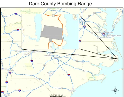
4.1 Study Area
The study area was located in the Dare County bombing range along the eastern
coast of North Carolina (Figure 1). The bombing range has been used by the United
States Air Force and Navy for air-to-surface target training and consists of 46,000 acres
of marshland, mixed forest land, low lying conifers, and open land. Atlantic white cedar
forest, pond pine woodland, cypress domes, streamhead pocosins, bay forest, basin
shrub-dominated types, and depression pocosins are the primary vegetation (Robinson et al.
1998). Only a few old-growth stands remain due to the heavy timber harvest of Atlantic
White Cedar during World War I. The bombing range was constructed in 1965 on land
leased from West Virginia Pulp and Paper. The Air Force obtained the range in 1978 and
has shared it with the Navy for use in training bomber pilots since then (Global Security
Figure 1: Study Area Location
4.2 Imagery
Images used for classification were 1: 6,000 color-infrared (CIR) aerial
photography of the Dare County bombing range flown during the spring of 2004. The
images were taken by Kucera International with a Kodak CIR 1443 camera with a focal
length of 152.850 mm at an altitude of 917 meters (3010 ft). Film positives were scanned
on a high quality consumer-grade Epson desktop scanning bed with a transparency unit
using 24-bit color at a resolution of 800 dots per inch (dpi) resulting in a nominal spatial
resolution of 19 cm (7.5 in) per pixel. Leica Photogrammetry Suite softcopy software
georectified Erdas Imagine files (Leica Geosystems 2006). Each file represented 418
acres on the ground and was 172-megabytes in size.
Based on visual inspection, ten images were selected for their similarity in color
variation and sun glint. We used Visual Learning System Inc.’s Feature Analyst (v
4.0.2.21) in ArcGIS 9.1 to classify areas of downed timber. To degrade the pixel
resolution of the original imagery we used the ‘degrade’ tool in Leica Geosystem’s Erdas
Imagine 8.7 that reduces the resolution of images. The actual process used to alter the
pixels is a proprietary technique that is not explicitly explained in the manual. User input
determines how far the pixel boundary is extended. The 0.2-meter resolution imagery
was degraded by a factor of five to create 1-meter resolution imagery. The spatial extent
of the original pixel was expanded horizontally and vertically by the specified integer
factor. Spectral values of the original pixel and surrounding pixels (within and adjacent
to the new spatial extent) were resampled to produce a new pixel with adjusted spectral
values. In the resampling process, spectral values of the original pixel were weighted
more heavily than those of surrounding pixels during the process and the relative
weighting increased as output pixel size increased (Leica Geosystems 2006).
4.3 Training Procedure
Our classification scheme was adapted from techniques developed by Miller
(2005) and Shedd et al. (2005). After examining the image, we determined that there
were three primary classes: downed timber, trees, and soil. We developed training sites
for each of the classes by hand-digitizing polygons that represented multiple examples of
considerable class confusion, especially within the tree and downed timber classes.
Although Feature Analyst provides clutter removal tools to modify existing
classifications and re-classify, modification attempts in this study compromised the
training set and decreased the ability to correctly classify the areas with downed timber.
Miller (2005) had the same problem with the clutter removal tools, finding the tools
could effectively improve the classification within an image but decreased the accuracy
of subsequent classifications of other images. Full descriptions of the imagery problems
encountered and software observations discovered during the training procedure can be
found in the appendix (Appendix 8.1).
To improve the classification over all images; more training polygons were added
for the confused classes. The downed timber and tree classes were also divided into
sub-classes because of the spectral variability within each primary class. The “downed
timber” class was divided into two subclasses: high amount of debris and low amount of
debris. Training classes that combined coniferous and deciduous trees increased the
classification run time and misclassified many areas, so the tree class was also subdivided
into deciduous and coniferous trees. An additional class was created for black film edges
and fiducial marks that were visible on individual images. There were a total of six
classes used in the object-oriented classification: high amount of debris downed timber,
low amount of debris downed timber, coniferous trees, deciduous trees, soil and photo
remnants.
The Feature Analyst software includes a series of preset wizard-driven options
that modify the classification algorithm to suit particular image types. These options
The options were (1) image band selection, (2) input representation, (3) inclusion of
rotated objects, (4) classification approach, and (5) aggregate areas.
1) Image band selection allows the user to specify which spectral bands are used and
whether the reflectance or texture should be used. The reflectance and texture of
all three input bands available were used in this study. Shedd et al. (2005) also
used reflectance and texture to classify downed timber. Reflectance refers to the
spectral qualities of the image and texture refers to the spectral uniformity of an
object. The inclusion of texture was instrumental in differentiating between soil
and individual tree stems. The spectral bands correspond to green, red and near
infrared reflectance.
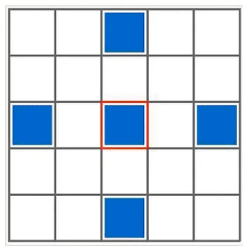
2) Input representation refers to the focal area used by the algorithm during
classification. The focal area helps define pattern and width of the area analyzed.
There are input representations that simulate the way that the human eye
recognizes different object patterns. Although there were many input
representations, we chose the one recommended by the ‘Feature Selector’ under
the ‘Learning Settings’ tab to identify natural features, ‘Bullseye 3’. Studies by
Shedd et al. (2005) and Miller et al. (2005) also used a ‘Bullseye’ input
representation to classify objects. A pattern width of thirty-three was used for the
.2 meter class covering an areas of 43.56 square meters (thirty-three 0.2-meter
pixels x thirty-three 0.2-meter pixels). A pattern width of 5 was used for the other
resolutions. At the 1-meter spatial resolution an area of 25 square meters would
not be reduced below five pixels and still maintain the input representation
pattern, so pattern width of 5 was used in all remaining classifications (Figure 2).
.2 meter meter spatial resolution 1, 5 and 10 meter spatial resolutions
Figure 2: Bullseye input representation
3) The option of including rotated objects allowed classification of downed trees no
matter which way they fell. If this option is not selected, the algorithm will only
classify downed timber that is in one orientation. For example, if the timber
specified in a training class lies at a forty-five degree angle, only downed timber
that falls at a forty-five degree angle will be classified.
4) There were three classification approaches available to determine how the
‘Learning Algorithm’ would classify the image. The default-learning algorithm,
Approach 1, was described as ‘general purpose;’ Approach 2 was described as
‘good for removing clutter;’ and Approach 3 was ‘quick but not as accurate.’
different approach for classifications, so the default, Approach 1 was selected as
the ‘Learning Algorithm.’
5) The ‘aggregate areas’ option controlled the size of the objects classified. By
selecting this option, we were able to eliminate areas that were too small to be
downed timber. The number of pixels to be aggregated changed inversely with
the pattern width (in pixels). At the 0.2-meter spatial resolution, there were
thirty-six pixels aggregated into objects. The number of pixels aggregated decreased to
five for all other spatial resolutions.
4.4 Classification
4.4.1 Object-Oriented
The first image was classified based on hand digitized training sites and algorithm
settings described previously. Each classification produced an ArcGIS shapefile and a
signature file that could be used to classify other images. Initially, each class had five
training sites with spectrally pure examples. After each classification, the classified
polygon was overlaid on the original imagery to determine how well the downed timber
areas were classified. Any areas that were missed or that were misidentified were noted
and adjustments to the training classes were made before the next classification attempt.
There are a few tools available with Feature Analyst that did not improve my
classification results. The ‘clutter removal’ tool was used to select portions of classified
polygons to be removed from the classification results and to specify which classified
could be added with the ‘add missed feature’ tool. However, these tools did not improve
the classification, but tended to confuse the algorithm. After using the clutter removal
tool, many areas that were not downed timber were erroneously added to the downed
timber class and areas that had been correctly classified as downed timber were removed.
Instead, training polygons were improved through the manual addition, deletion, and
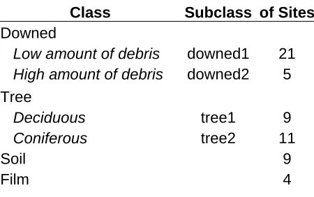
modification of training sites for each class. A total of fifty-nine training polygons were
used in the final classification (Table 1).
Table 1: Number of Training polygons by class used for initial learning algorithm
Class Subclass
Number of Sites
Downed
Low amount of debris downed1 21
High amount of debris downed2 5
Tree
Deciduous tree1 9
Coniferous tree2 11
Soil 9
Film 4
In order to classify all of the downed areas, each image was classified twice.
The batch process used the signature files for ‘downed1’ and ‘downed2’ to classify each
image independently. Two polygon shapefiles were produced for each image for a total
of twenty shapefiles at each spatial resolution. The twenty shapefiles were then merged
to create one shapefile at each of the four spatial resolutions. The remaining signature
files were not used to classify the images because we were only interested in classifying
4.4.2 Supervised Classification
I performed a supervised classification of the 1-meter spatial resolution dataset to
directly compare how a conventional classification approach and an object-oriented
classification. The software used for the supervised classification was Leica Geosystems
Erdas Imagine. I chose the 1-meter spatial resolution imagery because it had the highest
accuracy in the object-oriented classification. For direct comparison, the same training
polygons used for the object-oriented classification were used in the supervised
classification. Signature files for two ‘downed’ classes were used to classify all images
independently. Once all the images were classified, the shapefiles were merged together
to create one classified file for each spatial resolution.
4.4.3 Manual Classification
Areas of downed timber on the Dare County bombing range were also delineated
and classified manually using the aerial photography. An orthorectified mosaic was
created from all of the 0.2-meter imagery and used for the manual classification. The
minimum mapping unit was 1,000 square meters (0.1 hectare). The damaged areas were
categorized into three different classes based on damage: less than 30% damage, 30% to
60% damage, and greater than60% damage. Polygons were hand-digitized by two skilled
map technicians using heads-up digitizing. Areas were checked for accuracy using stereo
4.5 Accuracy Assessment
I conducted an accuracy assessment on the final classification of six data sets:
0.2-meter imagery, 1-0.2-meter imagery, 5-0.2-meter imagery, 10-0.2-meter imagery, manual
delineation, and supervised classified data. Based on Congalton’s (1999)
recommendation of 250 points with a minimum of 50 points per class, I created a new
point shapefile with 300 randomly generated points and ensured that there were at least
125 points per class (Congalton and Green 1999). Because the final classified maps
consisted of two categories, downed timber and other, each point was labeled as ‘downed
timber’ or ‘other’ by visual comparison to the original 0.2-meter scanned imagery. Once
all of the points were classified, we counted the number of ‘downed timber’ reference
points that fell within areas classified as ‘downed timber’ and the number of ‘other’
reference points that fell within areas not classified as ‘downed timber.’
Overall accuracy, user’s accuracy, producer’s accuracy, a kappa statistic, kappa
variance and kappa z statistic were calculated (Congalton and Green 1999). The overall
accuracy of each classification was determined by dividing the total number of points
correctly classified by the total number of reference points. The user’s accuracy,
calculated by dividing the total number of correct points in a class by the total number of
points classified in that class, estimates the probability that the classified point on the
map actually represents that category on the ground. The producer’s accuracy, calculated
by dividing the total number of correct points in a class by the total number of reference
points in that class, estimates the probability that a point in a particular category is
correctly classified. The kappa statistic was generated to describe the agreement between
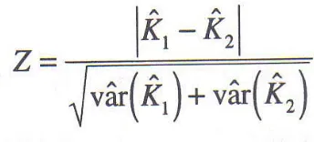
(Figure 3) and kappa variance were based on the kappa statistic and were used in a test to
determine if two error matrices were significantly different (Congalton and Green 1999).
This pair-wise test compared error matrices two at a time to determine if they were
significantly different from one another (Figure 4).
K1 = kappa statistic for an individual error matrix
Figure 3: Kappa z statistic computation
K1 = kappa statistic for an individual error matrix
K2 = kappa statistic for an individual error matrix
Figure 4: Z statistic test computation
5. Results
5.1 Accuracy
The final thematic maps had two classes: areas with downed timber and other
areas. The accuracy at each spatial resolution varied from 58% for the manual
delineation to 86% for the 1-meter classification (Table 2). The 1-meter resolution
with respect to the ‘downed timber’ class, and the highest user’s accuracy with respect to
the ‘other’ classification; the kappa statistic was also the highest for this resolution (Table
3). The 5-meter classification had the highest user’s accuracy with respect to ‘downed
timber’ and the highest producer’s accuracy with respect to ‘other area’.
A kappa statistic value greater than 0.8 indicates a strong level of agreement
between the classified and reference data (Jensen 2005). The kappa statistic for each of
the thematic maps demonstrated a moderate level of agreement between classification
results using Feature Analyst because all fell between 0.4 and 0.8 (Jensen 2005). The
kappa z-test was used to indicate superiority of one set of classification results over
another. All of the object-oriented classifications had a higher kappa z – statistic than the
supervised classification and the 1-meter classification was the highest (Table 2).
However, the difference test did not show a significant difference (z > 1.96) among
object-oriented classifications at different spatial resolution, but there were significant
differences between the supervised classification, the manual delineation and the
object-oriented classifications (Table 3). Overall, the 1-meter classification outperformed the
other classifications, but none of the differences were statistically significant within
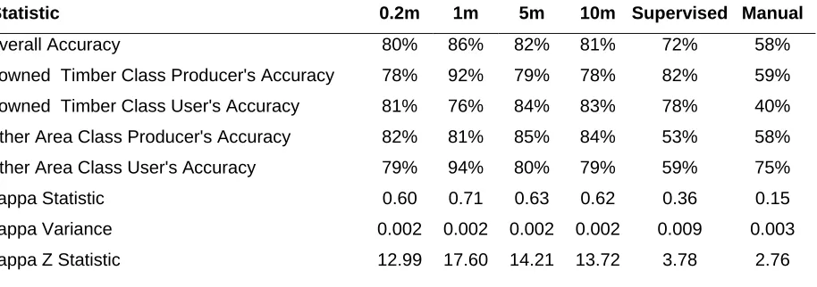
Table 2: Summary of the classification accuracy results.
Statistic 0.2m 1m 5m 10m Supervised Manual
Overall Accuracy 80% 86% 82% 81% 72% 58%
Downed Timber Class Producer's Accuracy 78% 92% 79% 78% 82% 59%
Downed Timber Class User's Accuracy 81% 76% 84% 83% 78% 40%
Other Area Class Producer's Accuracy 82% 81% 85% 84% 53% 58%
Other Area Class User's Accuracy 79% 94% 80% 79% 59% 75%
Kappa Statistic 0.60 0.71 0.63 0.62 0.36 0.15
Kappa Variance 0.002 0.002 0.002 0.002 0.009 0.003
Kappa Z Statistic 12.99 17.60 14.21 13.72 3.78 2.76
Table 3: Z statistic test between matrices.
A value greater than 1.96 indicates a statistically significant difference between classifications
0.2 m 1 m 5 m 10 m Supervised Manual
0.2 m NA 1.80 0.53 0.32 2.27 6.28
1 m 1.80 NA 1.27 1.48 3.39 8.24
5 m 0.53 1.272 NA 0.21 2.60 6.85
10 m 0.32 1.48 0.21 NA 2.47 6.62
Supervised 2.27 3.39 2.60 2.47 NA 1.91
Manual 6.28 8.24 6.85 6.62 1.91 NA
0% 25% 50% 75% 100% Overall Accuracy Downed Timber Class Producer's Accuracy Downed Timber Class User's Accuracy Other Area Class Producer's Accuracy Other Area Class User's Accuracy .2m 1m 5m 10m Supervised Manual
5.2 Maps
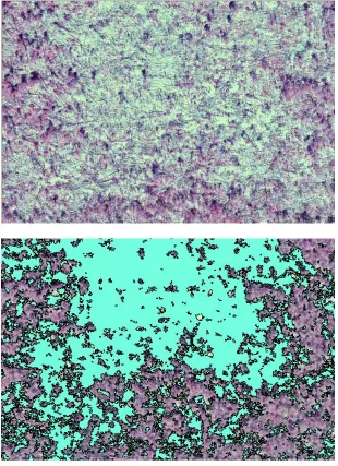
Using Feature Analyst, we were able to generate five thematic maps representing
four spatial resolutions and the supervised classification. Each thematic map consists of
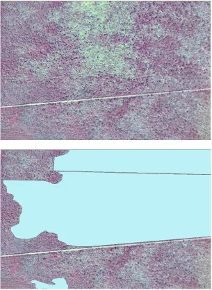
‘downed timber’ polygons and ‘other area’ polygons (Figure 6 and 7). Top images are a
portion of the area classified and bottom images include light blue polygons representing
downed timber areas overlaid on the image above.
Figure 6: Original 0.2-meter image and classification
Figure 7. 1-meter image and classification
5.3 Area Comparison
As a further comparison of the manual classification to digital classifications at
different spatial resolutions, we decided to compare estimated total area of downed
timber in each. The computer-based classifiers evaluated the imagery at a pixel level that
manual delineation could not reach, so we also compared the relative size of the polygons
in each classification. Polygons in the manual classification (Figure 8) were much larger
than the computer classifications (Figure 6 and 7) and had fewer vertices, which made the
polygon much more generalized. Polygons delineated manually contained damaged
areas and undamaged areas, whereas the polygons derived digitally only contained
damaged areas. Therefore the damaged area estimated by the manual classification was
much larger than the acreage estimated from the computer-based classifications (Table 4
and Figure 9).
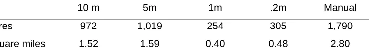
Table 4: Area of the downed timber estimated using different resolution imagery and
manual classification
10 m 5m 1m .2m Manual
Acres 972 1,019 254 305 1,790
Figure 8. Original image and manual classification
0 500 1,000 1,500 2,000
10 m 5m 1m .2m Manual
Figure 9: Total downed timber area comparison for different resolutions of classified
images and manual delineation.
6. Discussion of Results
Hypothesis 1. An object-oriented classification can be used to accurately identify and
classify downed timber on high-resolution imagery.
We found that an object-oriented classification can be used to identify downed timber on
high-resolution aerial photography and that the classifications can be replicated on other
images.
Hypothesis 2. The classification can be replicated for images with similar
characteristics.
The training data I created on one image and used to classify the remaining images
Hypothesis 3. Feature Analyst can be used at variable resolutions to identify downed
timber.
Classification accuracy and kappa statistics demonstrated that downed timber areas can
be identified at different spatial resolutions with an object-oriented classification
technique (Table 3).
Hypothesis 4. Feature Analyst’s results are similar to results achieved through a
pixel-based supervised classification and a manual delineation.
Using an object-oriented approach, classification accuracies at different spatial
resolutions were not statistically different from each other, but were significantly
different than results from manual delineation and conventional supervised classification
approaches.
Before the accuracy assessment began, we anticipated that the classification
produced by the 0.2-meter imagery would be the most accurate due to the high level of
detail in the imagery. Although the classification results produced from the 5-meter and
10-meter imagery appeared to be coarse, statistically there was no difference between the
object-oriented classifications at different spatial resolutions (Table 3).
The accuracy assessments provided a quantitative estimate of the success of each
classification, but did not account for the visual quality of the classification. Visual
comparison of each classification shows a reduction in number of polygons and increase
in size of polygons as spatial resolution is decreased. Changes in the polygons are
noteworthy. In the 0.2-meter imagery, the polygons are smaller, more numerous and
have complex edges. Each polygon has a large number of vertices. The polygons
classification, which softened some of the rough edges and reduced the number of
smaller polygons, thereby reducing the “salt and pepper” appearance of the classification.
The 5-meter classification looked “blocky” with larger pixels visible and polygon edges
with ninety-degree angles. The 10-meter classification loses many of the smaller downed
areas and exhibits more “blocky” appearance than the 5-meter classification.
Overall, the object-oriented classification approach was able to meet the challenge
of identifying downed timber in an accurate and reasonably efficient manner. The level
of detail and file size of the 0.2-meter pixel imagery increased classification runtime and
required more attention to detail with respect to developing training sites. Classifying the
0.2-meter classification took an average of thirty-five minutes per image, yet the entire
set of 10-meter imagery took twenty minutes. As the spatial resolution was degraded, the
file size of the images decreased from 171 MB at 0.2-meter to 7 MB at 1-meter to 317 kb
at 5-meter to 124 kb at 10-meter. There were fewer polygons with less detail classified
as the spatial resolution increased from the original 0.2-meter resolution, yet the accuracy
was not affected by this reduction. The file size on the 1-meter classification also
decrease from the 0.2-meter classification (8,174kb vs 472,607 kb).
The object-oriented classifications were significantly different from the manual
delineation and the supervised classification, but the supervised classification was not
significantly different from the manual delineation. The lower accuracy of the supervised
classification was most likely the result of spectral confusion between ‘soil’ and ‘downed
timber’; these classes were confused more often in the supervised classification than in
the object-oriented classification. The object-oriented classification incorporated
Although the selection of 1-meter, 5-meter and 10-meter imagery was made to
simulate available satellite sensors, the 0.2-meter imagery was actually acquired from an
airborne camera rather than a satellite sensor. The initial 0.2-meter classification took a
long time to produce because of the significant amount of time spent learning to operate
Feature Analyst. Once the proper technique was developed, the classification was much
quicker than manual, hand-delineated classification of the data. Manual classification of
the area took nearly five hours while the 1-meter object-oriented classification took an
hour and a half. The level of detail provided by the object-oriented classification was
much greater than the manual classification and explains much of the disparity in total
area calculation between object-oriented and other classifications. The difference in area
among the object-oriented classifications at different spatial resolutions was most likely
relative to the pixel size difference. Although downed timber areas consisted of several
pixels for each spatial resolution, difference in pixel size increased the downed timber
area estimates because the degraded pixels covered more area and consisted of more than
just downed timber. Although the number of pixels that comprise an object is five pixels,
the area of those objects increase from 25 square meters to 100 square meters as spatial
resolution increased from 5-meter to 10-meter. There were multiple polygons generated
by the object-oriented classification in each polygon manually classified. The manual
classification polygons were much larger than those generated by the object-oriented
classification since manual delineation tends to captures undamaged area along with
downed timber. The ‘downed timber’ polygons from the object-oriented classification
The same training polygons that were created on, and used to classify the
0.2-meter classification, were used to generate training data at all other spatial resolutions.
Originally, the decision to use the same training polygons on every spatial resolution was
made to avoid a bias in training data selection. However, the lack of significant
difference among object-oriented classifications demonstrates that it is possible to use
training polygons created on high-resolution imagery to generate training data on coarser
resolution imagery. This technique can decrease the cost of natural disaster damage
assessment by reducing the need for high-resolution imagery for the entire affected area.
Instead, high-resolution imagery can be acquired for a portion of the affected area and
used to generate training data to classify coarser resolution imagery over the larger area.
Computer required to store and manipulate coarse resolution imagery would be less
expensive to acquire and easier to manipulate because of smaller file sizes. Further study
is needed to determine if this technique is applicable to other types of imagery at other
spatial resolutions.
In conclusion, the classification accuracies demonstrated that object-oriented
classification techniques can successfully identify downed timber areas. However, after
comparing the results of the classifications, there was no statistically significant
difference among the object-oriented classifications, but there was a significant
difference between the object-oriented results and the other classifications. Using the
training data created on the high-resolution imagery to classify the coarser spatial
resolution imagery did not cause classification accuracy to diminish. The potential
damage assessment impact of this technique is that low-resolution imagery can be
create training data. High-resolution imagery is more expensive and requires more disk
space to store. Low-resolution imagery is less expensive and has a smaller file size,
making it easier to manipulate. Remote sensing damage assessment is more appealing to
government agencies as a less expensive, quick method to acquire the data necessary to
quantify damaged areas and focus recovery efforts. This classification technique
demonstrates that damage assessment can be accomplished less expensively, without
sacrificing accuracy and speed.
7. List of References
Adams B. 2005 March. “Remote Sensing Technology- A Coming of Age.” Natural Hazards Observer 29:4.
Adams B. 2005. “Remote Sensing Technology for Response and Recovery”, Multidisciplinary Center for Earthquake Engineering Research.
Akgün A, Eronat AH, Turk, N. 2004. Comparing Different Satellite Image
Classification Methods: An Application In Ayvalýk District,Western Turkey. XXth International Congress for Photogrammetry and Remote Sensing, Proceedings, Ýstanbul,Turkey.
Anonymous. 2007. Tropical cyclone. URL= http://en.wikipedia.org/wiki/Hurricane, visited 2007 May 16.
Berg, E C. 2004. Survivorship and Growth of Oak Regeneration in Wind-Created Gaps Gen. Tech. Rep. SRS-73. Asheville, NC: U.S. Department of Agriculture, Forest Service, Southern Research Station. pp. 143-149.
Berg, EC, Van Lear, DH. 2004. Yellow-Poplar and Oak Seedling Density
Responses to Wind-Generated Gaps Gen. Tech. Rep. SRS–71. Asheville, NC: U.S. Department of Agriculture, Forest Service, Southern Research Station. pp. 254-259.
Benson BJ, MacKenzie, MD. 1995. Effects of sensor spatial resolution on landscape structure parameters - Landscape Ecology, 1995 – Springer
Landscape Ecology vol. 10 no. 2 pp 113-120.
Benz U, Hofmann P, Willhauck G, Lingenfelder I, Heynen M.
M. 2004. Multi-resolution, object-oriented fuzzy analysis of remote sensing data for GIS-ready information. ISPRS Journal of Photogrammetry and Remote Sensing 58:239-258.
Blaschke T, Lang S, Lorup E, Strobl J, Zeil P. 2000. Object-oriented image
processing in an integrated GIS/remote sensing environment and perspectives for environmental applications. In: Cremers, A. und Greve, K. (Hrsg.):
Umweltinformation für Planung, Politik und Öffentlichkeit / Environmental Information for Planning, Politics and the Public. Metropolis Verlag, Marburg, vol 2; 555–570.
Blaschke T, Strobl J. 2001. What’s wrong with pixels? Some recent developments interfacing remote sensing and GIS. GeoBIT/GIS, 6, 12– 17.
Congalton, R. and K. Green. 1999. Assessing the Accuracy of Remotely Sensed Data: Principles and Practices. CRC/Lewis Press, Boca Raton, FL. 47-53 p.
Global Security. 2007. Dare County Range (R-5314). URL =
http://www.globalsecurity.org/military/facility/dare-county.htm, visited 2007 May 16
Greenberg CH, McNab WH. 1997. Forest Disturbance in hurricane
related downbursts in the Appalachian mountains of North Carolina. Forest Ecology and Management 199X: 179-191.
Jackson RG, Foody GM, Quine CP. 2000. Characterising windthrown gaps from fine spatial resolution remotely sensed data. Forest Ecology Management. 135: 253-260.
Jensen J R. 2005. Introductory Digital Image Processing; A Remote Sensing Perspective. Upper Saddle River, NJ: Prentice Hall. p 337-339.
Kaya S, Musaoglu N, Ormeci G, Muftugulu. 1998. Forest damage assessment by using remote sensing data. IAPRS 32(4): 284-287.
Laliberte A, Rango A, Fredrickson, EL. 2005. Classification of arid rangelands using an object-oriented and multi-scale approach with Quickbird imagery. Proceedings of the American Society for Photogrammetry and Remote Sensing Annual
Conference, March 7-11, 2005, Baltimore, Maryland. 2005 CDROM.
Leica Geosystems. Erdas Imagine 8.7. 2006. URL =
home.gdal.org/projects.imagine.iau_docu1.pdf visited 2006 November 11.
Lillesand TM, Kiefer RW, Chipman JW. 1994. Remote Sensing and Image Interpretation third ed. New York: John Wiley and Sons INC. p 629-634.
Merrens EJ, Peart DR. 1992. Effects of hurricane damage on
individual growth and stand structure in a hardwood forest in New Hampshire, USA. Journal of Ecology 80: 787-795.
Miller J, Nelson S, Hess G, 2005. A new object-oriented method of
impervious surface classification using Feature Analyst [thesis]. Raleigh (NC): North Carolina State University.
Nelson, DM. 2004. Remote Sensing Classification of Brownsfields in the Phoenix Metropolitan Area. International Society of Photogrammetry and Remote
Parson A, Orlemann A. 2002. Mapping Post-Wildfire Burn Severity Using
Remote Sensing and GIS, ESRI Conference 2002, USDA Forest Service, Remote Sensing Applications Center, Salt Lake City, UT.
Polngam S. 2005. Remote Sensing Technology for Tsunami Disasters along the Andaman Sea, Thailand. Geo-Informatics and Space Technology Development Agency, International Workshop on the Application of Remote Sensing
Technologies in Earthquake Damage Assessment. September 12-13 2005, Japan.
Redmond R, Winne JC, Opitz D, Mangrich MV. 2001. Classification and Mapping Wildfire Severity. Imaging Notes 16:24-25.
Rejaie A, Shinozoka M. 2003. Urban Damage Assessment from Remotely Sensed Images. URL =
http://www.mceer.buffalo.edu/publications/sp_pubs/01-SP02/sra_ind/08.pdf. visited 2003 March 10.
Schwarz M, Steinmeier C, Holecz F, Stebler O, Wagner H. 2003. Detection of
Windthrow in Mountainous Regions with Different Remote Sensing Data and Classification Methods. Scandanavian Journal of Forest Research 18: 525-536.
Shedd J, Millinor B, Devine H. 2005. Updating Fuel Fire Loads and Vegetation Datasets after a Natural Disaster [thesis]. Raleigh (NC):North Carolina State University.
Vanderzanden D, Morrison M. 2002. High Resolution Image Classification: A
Forest Service Test of Visual Learning System’s Feature Analyst. USDA-Forest Service Remote Sensing Applications Center, Salt Lake City UT 84119.
Visual Learning System. Visual Learning Systems Feature Analyst
4.0 Reference Manual. 2004. URL = http://www.featureanalyst.com. visited 5 February 2006.
8. Appendix
8.1 Discussion on the Imagery
Variable imagery quality issues caused many problems for Feature Analyst. In
this study, the image quality varied between flight lines, images in each flight line, and
within each image. Mosaics were generated to attempt to solve some of the quality issues
and produce a uniform and consistent image to be classified. However, the mosaics often
produced lower quality imagery due to the considerable variability described above. The
mosaics lost spectral clarity and became grainy as Leica Geosystem Inc.’s Erdas Imagine
attempted to generate a uniform consistency throughout. This lack of quality combined
with the size of the images severely compromised the quality of the classification results
produced by Feature Analyst. Often the classification runs would take several hours to
compile and when finished would produce memory errors that would cause ArcMap to
terminate and lose the entire set of data. The lean of the trees and sunspots on the images
would generate false positive results during classifications. The exposed tree trunk of a
tree exhibiting severe lean would be classed as downed timber and sun spots or glint
would appear to be clearings of downed timber.
8.2 Discussion of Software
Feature Analyst proved to be effective object-oriented classification software, but
it was not without its difficulties. There was a considerable learning curve with the
package comes with a variety of wizard developed tools and menus, there are many
topics that need to be discussed and solved before any classification job is attempted.
The Feature Analyst object-oriented classification approach was most effective
when there were enough training classes to represent all of the objects that could be
found on the image. In this study, using one training class (downed timber) to classify
the entire image did not work effectively. Exporting one class from a complete
classification works well, but simply classifying one class in the beginning does not.
Based on this reasoning, it is important to add as many training sets and classes to
classify a majority of the image before attempting to classify an image. When the “wall
to wall” option was selected, objects that did not fall within specified training classes
were forced into the class that it was most similar to. While this may produce a
classification for the whole image, in this study we found that it actually confused the
classifying algorithm in Feature Analyst because it forced unknown areas into one or
more classes and diluting the quality of the classified polygons. Not selecting the “wall
to wall” option produced a thematic map with polygons of pure downed timber rather
than mixed polygons. Training polygons could then be refined or augmented to produce
the desired results.
Originally, the concept was to use an object-oriented classification to identify and
classify the actual timber stems and root bundles. After several attempts, we realized that
the varied color, texture, shape, and size of the downed timber proved too complex for
accurate classification at the original spatial resolution. The individual timbers were
confused with any tree that was upright and exposed as well as patches of soil and in
were made to change and add polygons to the training sites in hopes of eliminating this
class confusion. Different input representations and pattern widths were also used to try
and find any that would be able to identify the downed timber stems. Running multiple
classifications on the particular image to “mask” out areas that definitely were not
downed timber and to concentrate the search in areas that definitely had downed timber
did not improve the results.
I also tried increasing and decreasing the size of the image being classified to
reduce the variability among images and across the imagery, yet the results did not
improve. Classifying more than one image at a time increased classification run times and
introduced new classification errors and omissions. Many computer related problems
occurred including, unexpected crashing, loss of data and freezing by increasing the
image size. Reducing the image size decreased the run time but had little to no effect on
the quality of the classification. The smaller images did not produce training examples
that could be used to classify other images or even the rest of the image that the training
polygons were taken from.
8.3 Solutions
To solve these imagery and software problems, I classified areas with downed
timber and used a select group of original images. By classifying areas with downed
timber instead of individual timbers, I was able to take advantage of contextual
object-oriented classification system in Feature Analyst. Including texture of the objects in the
classification allowed Feature Analyst to differentiate between groups of downed trees
that made up downed timber in a pixel-based classification, but combining the edges and
shadows that surrounded areas with downed timber proved to make the difference.
Classifying areas instead of individual trees also helped eliminate the classification of
tree trunks that were exposed.
Selecting images that had similar sun glint and tree lean had a dramatic effect on
the quality of the classification possible and especially the ability to batch classify
multiple images. There were a total of thirty-nine images that contained downed timber
in the study area. Of those thirty-nine, ten images were selected that had similar image
quality with respect to lean, glint and pixilation or sharpening. Taking advantage of the
richness of the raw imagery rather than allowing a mosaic to wash out the images,
provided an adequate amount of data to produce complete classifications. Using one
image, also significantly reduced the run time on each classification. Once the signature
files were generated for each spatial resolution, batch classification took less time and
caused no computer related problems.
There were considerable problems and issues that occurred during this study.
Feature Analyst, as an ArcGIS extension, is fairly hardy, but there are many quirky parts
of the program that can give beginners problems. Using training files, for example can
problematic if you begin working on different drives. Much of the study data were
housed on a personal hard drive and much of the processing was accomplished on North
Carolina State University lab computers. In order to use signature files that were
generated on previous classification runs, the classified polygon shapefiles for which they
were generated must be on the drive that housed the signature file. If the signature file
the batch classification would fail and produce an error stating that there was “no training
data” to run the classification on. To avoid this error, I create a new input combination
file, run the classification and split the files out just prior to the classification run instead
of using data generated earlier. It was also important to pay attention to the origin of the
signature file. Batch classification generates signature files for the new classifications,
but they cannot be used for batch classification later. Those signature files generate the
same “no training data” available error mention earlier.
Another important consideration when using archival data is that any file
generated by a tool in the Feature Analyst toolbar, including multiclass input layers,
clutter removal files, combined feature and classification results, loses its symbology if it
is not saved and kept in the .mxd file that created it. Feature Analyst must maintain the
symbology in the .mxd file and not in the actual file. This is another reason to only work
within in one .mxd file for each complete classification run.
8.4 Recommendations
8.4.1 Image Specific
In order to truly harness the full potential of an object-oriented classification
software like Feature Analyst, image quality is critical. If there is one universal truth
exposed by this study it is that imagery quality controls the quality of the classification,
the level of difficulty in developing training data, and the time necessary to complete
classification. Many of the pitfalls and problems developed ultimately from poor
and color variations within images. When classifying objects rather than individual
pixels, the size is not nearly as important as the recognition of that object.
8.4.2 Feature Analyst Specific
In this study, downed timber areas could be classified on the five spatial
resolutions by using Feature Analyst. However, using Feature Analyst may not solve all
classification needs. The best use for Feature Analyst is to identify objects that are
relatively similar in all images and relatively homogenous. Using Feature Analyst to
classify heterogeneous objects may be only partially successful unless the objects are in
different training classes. The software has a wealth of options and settings that need to
be explored before selecting one particular technique. Band selection, approach selection
and input representation have a plethora of possibilities that can be used. Being mindful
of the spatial resolution is also important when selecting the best input representation.
This selection should be modified based on the size of the object that is to be classified.
In this study, we were looking for downed timber and once the pixel size and
subsequently the input representation started to be larger than the object being classified;
the quality of the classification decreased. Overall, the Feature Analyst software package
is a relatively robust classifier with its own limitations and advantages. Although it has
seemed that the remotely sensed imagery technology has outpaced the classification
software, classification technology will close the gap through the advancement of
Figure 10. Set up learning options for Feature Analyst
Figure 12. Input representation for 0.2-meter classification