University of Windsor University of Windsor
Scholarship at UWindsor
Scholarship at UWindsor
Electronic Theses and Dissertations Theses, Dissertations, and Major Papers
2013
Bayesian Spatial Additive Hazard Model
Bayesian Spatial Additive Hazard Model
Alexander Chernoukhov
University of Windsor
Follow this and additional works at: https://scholar.uwindsor.ca/etd
Recommended Citation Recommended Citation
Chernoukhov, Alexander, "Bayesian Spatial Additive Hazard Model" (2013). Electronic Theses and Dissertations. 4965.
https://scholar.uwindsor.ca/etd/4965
This online database contains the full-text of PhD dissertations and Masters’ theses of University of Windsor students from 1954 forward. These documents are made available for personal study and research purposes only, in accordance with the Canadian Copyright Act and the Creative Commons license—CC BY-NC-ND (Attribution, Non-Commercial, No Derivative Works). Under this license, works must always be attributed to the copyright holder (original author), cannot be used for any commercial purposes, and may not be altered. Any other use would require the permission of the copyright holder. Students may inquire about withdrawing their dissertation and/or thesis from this database. For additional inquiries, please contact the repository administrator via email
Bayesian Spatial Additive Hazard Model
by
Alexander Chernoukhov
A Thesis
Submitted to the Faculty of Graduate Studies
through the Department of Mathematics and Statistics
in Partial Fulfillment of the Requirements for
the Degree of Master of Science at the
University of Windsor
Windsor, Ontario, Canada
2013
c
Bayesian Spatial Additive Hazard Model
by
Alexander Chernoukhov
APPROVED BY:
—————————————————————–
A. Ngom
School of Computer Science
—————————————————————–
M. Hlynka
Department of Mathematics and Statistics
—————————————————————–
A. Hussein, Advisor
Department of Mathematics and Statistics
—————————————————————–
S. Nkurunziza, Advisor
Department of Mathematics and Statistics
iii
Author’s Declaration of Originality
I hereby certify that I am the sole author of this thesis and that no part of this
thesis has been published or submitted for publication.
I certify that, to the best of my knowledge, my thesis does not infringe upon
anyone’s copyright nor violate any proprietary rights and that any ideas, techniques,
quotations, or any other material from the work of other people included in my
thesis, published or otherwise, are fully acknowledged in accordance with the standard
referencing practices. Furthermore, to the extent that I have included copyrighted
material that surpasses the bounds of fair dealing within the meaning of the Canada
Copyright Act, I certify that I have obtained a written permission from the copyright
owner(s) to include such material(s) in my thesis and have included copies of such
copyright clearances to my appendix.
I declare that this is a true copy of my thesis, including any final revisions, as
approved by my thesis committee and the Graduate Studies office, and that this thesis
iv
Abstract
This thesis will be dealing with the problem of Bayesian estimation in additive
survival data models accounting for spatial dependencies.
We consider the Aalen’s additive hazards model in which baseline hazard function,
the regression coefficients as well as the covariates are all allowed to be time varying
processes. We incorporate in this model an extra random vector of frailties accounting
for spatial variations among the observations.
Consequently, we propose a Bayesian approach to solving the inference problem
for such spatial frailty model by assuming piece-wise constant structure on all
time-varying functions in the model and hence, imposing appropriately chosen priors on
all model parameters.
We then employ some versions of MCMC and Gibbs sampling approaches to carry
out the inference about the model parameters and apply the resulting algorithm to
Prostate cancer diagnosis data for the state of Louisiana, taken from the Surveillance,
v
Acknowledgements
I would like to express my gratitude to my supervisors Dr. A. Hussein and Dr.
S. Nkurunziza. I want to thank them for valuable comments and suggestions. They
supported me both with choosing the research direction and overcoming the technical
issues. Also they gave me the opportunities to work independently which allowed me
to learn a lot of material from different fields of Mathematics and Statistics and
improve the problem solving skills.
Also I want to thank University of Windsor, Department of Mathematics and
Statistics and my supervisors for providing me with Research and Graduate
Assis-tantships. This financial support allowed me to concentrate on studying and finish
my program at this wonderful university.
I also want to thank my friends in Canada who supported me during the whole
year and showed me the Canadian traditions and sights.
And I want to thank my wife very much for her invaluable contribution into my
life. She constantly supported and helped me with any difficulties and problems
which I encountered since we met. She was always there for me when I needed it
and I learned a lot of important things from her. Her support allowed me to come to
Canada and successfully finish my study and I believe it will help me to succeed in
Contents
Author’s Declaration of Originality iii
Abstract iv
Acknowledgements v
List of Tables viii
List of Figures ix
Chapter 1. Introduction 1
1. Literature review 1
2. Thesis objectives and organization 3
Chapter 2. Additive Hazard Model with Conditional Autoregressive Spatial
Structure 6
1. Additive hazard frailty model 6
2. Model specification 9
3. Posterior distribution 20
4. Obtaining random sample from the posterior distribution 21
Chapter 3. Geostatistical spatial model 41
1. Prior distribution for the geostatistical model 41
CONTENTS vii 2. Obtaining a random sample from the posterior distribution 44
Chapter 4. Application of the Method 48
1. Model Implementation 48
2. Simulation Study 50
3. Application to the Prostate Cancer Data 55
Chapter 5. Conclusions 68
Appendix A. Introduction to Markov Chain Monte Carlo 70
1. Gibbs sampler 70
2. Metropolis-Hastings step 72
Appendix B. Proofs of Propositions Concerning Full Conditional Distributions 76
1. Baseline full conditional distribution 76
2. Regression function full conditional distribution 81
3. Frailty full conditional distribution 86
Appendix C. Modified Newton-Raphson Algorithm for Finding the Extremum
in an Open Interval 91
Appendix D. Results of Simulations 93
Bibliography 118
List of Tables
1 Variables Used in Data Analysis 55
2 Values of DIC, pD and LCP O for different numbers of intervals 60
List of Figures
1 Comparing real and proposal distribution for sampling from the full
conditional of the baseline 25
1 Continuation: Comparing real and proposal distribution for sampling from
the full conditional of the baseline 26
2 Comparing real and proposal distribution for sampling from frailty’s full
conditional 38
3 Estimated Parameters of The Model 62
4 Estimated Parameters of The Model (Continuation) 63
5 Estimated Parameters of The Model (Continuation) 64
6 Estimated Parameters of The Model (Continuation) 65
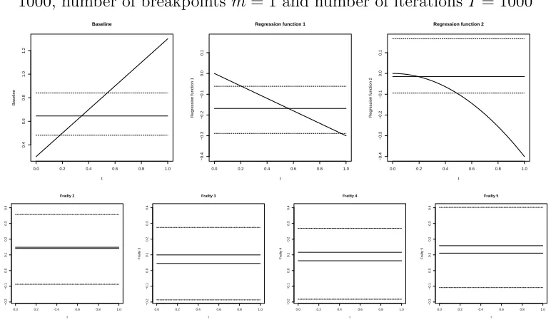
7 Estimated parameters for number of observations N = 100, number of
breakpoints m= 1 and number of iterationsI = 100 93
8 Estimated parameters for number of observations N = 100, number of
breakpoints m= 1 and number of iterationsI = 500 94
9 Estimated parameters for number of observations N = 100, number of
breakpoints m= 1 and number of iterationsI = 1000 94
LIST OF FIGURES x 10 Estimated parameters for number of observations N = 100, number of
breakpoints m= 1 and number of iterationsI = 5000 95
11 Estimated parameters for number of observations N = 100, number of
breakpoints m= 5 and number of iterationsI = 100 96
12 Estimated parameters for number of observations N = 100, number of
breakpoints m= 5 and number of iterationsI = 500 96
13 Estimated parameters for number of observations N = 100, number of
breakpoints m= 5 and number of iterationsI = 1000 97
14 Estimated parameters for number of observations N = 100, number of
breakpoints m= 5 and number of iterationsI = 5000 97
15 Estimated parameters for number of observations N = 100, number of
breakpoints m= 10 and number of iterations I = 100 98
16 Estimated parameters for number of observations N = 100, number of
breakpoints m= 10 and number of iterations I = 500 98
17 Estimated parameters for number of observations N = 100, number of
breakpoints m= 10 and number of iterations I = 1000 99
18 Estimated parameters for number of observations N = 100, number of
breakpoints m= 10 and number of iterations I = 5000 99
19 Estimated parameters for number of observations N = 100, number of
LIST OF FIGURES xi 20 Estimated parameters for number of observations N = 100, number of
breakpoints m= 50 and number of iterations I = 500 100
21 Estimated parameters for number of observations N = 100, number of
breakpoints m= 50 and number of iterations I = 1000 101
22 Estimated parameters for number of observations N = 100, number of
breakpoints m= 50 and number of iterations I = 5000 101
23 Estimated parameters for number of observations N = 1000, number of
breakpoints m= 1 and number of iterationsI = 100 102
24 Estimated parameters for number of observations N = 1000, number of
breakpoints m= 1 and number of iterationsI = 500 102
25 Estimated parameters for number of observations N = 1000, number of
breakpoints m= 1 and number of iterationsI = 1000 103
26 Estimated parameters for number of observations N = 1000, number of
breakpoints m= 1 and number of iterationsI = 5000 103
27 Estimated parameters for number of observations N = 1000, number of
breakpoints m= 5 and number of iterationsI = 100 104
28 Estimated parameters for number of observations N = 1000, number of
breakpoints m= 5 and number of iterationsI = 500 104
29 Estimated parameters for number of observations N = 1000, number of
LIST OF FIGURES xii 30 Estimated parameters for number of observations N = 1000, number of
breakpoints m= 5 and number of iterationsI = 5000 105
31 Estimated parameters for number of observations N = 1000, number of
breakpoints m= 10 and number of iterations I = 100 106
32 Estimated parameters for number of observations N = 1000, number of
breakpoints m= 10 and number of iterations I = 500 106
33 Estimated parameters for number of observations N = 1000, number of
breakpoints m= 10 and number of iterations I = 1000 107
34 Estimated parameters for number of observations N = 1000, number of
breakpoints m= 10 and number of iterations I = 5000 107
35 Estimated parameters for number of observations N = 1000, number of
breakpoints m= 50 and number of iterations I = 100 108
36 Estimated parameters for number of observations N = 1000, number of
breakpoints m= 50 and number of iterations I = 500 108
37 Estimated parameters for number of observations N = 1000, number of
breakpoints m= 50 and number of iterations I = 1000 109
38 Estimated parameters for number of observations N = 1000, number of
breakpoints m= 50 and number of iterations I = 5000 109
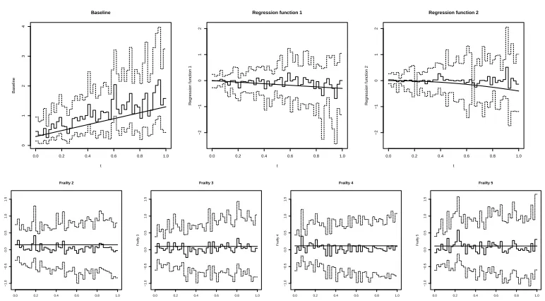
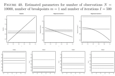
39 Estimated parameters for number of observations N = 10000, number of
LIST OF FIGURES xiii 40 Estimated parameters for number of observations N = 10000, number of
breakpoints m= 1 and number of iterationsI = 500 110
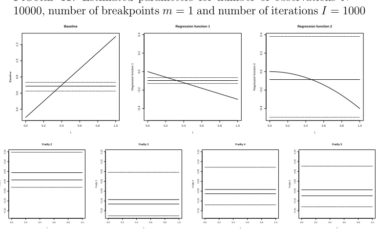
41 Estimated parameters for number of observations N = 10000, number of
breakpoints m= 1 and number of iterationsI = 1000 111
42 Estimated parameters for number of observations N = 10000, number of
breakpoints m= 1 and number of iterationsI = 5000 111
43 Estimated parameters for number of observations N = 10000, number of
breakpoints m= 5 and number of iterationsI = 100 112
44 Estimated parameters for number of observations N = 10000, number of
breakpoints m= 5 and number of iterationsI = 500 112
45 Estimated parameters for number of observations N = 10000, number of
breakpoints m= 5 and number of iterationsI = 1000 113
46 Estimated parameters for number of observations N = 10000, number of
breakpoints m= 5 and number of iterationsI = 5000 113
47 Estimated parameters for number of observations N = 10000, number of
breakpoints m= 10 and number of iterations I = 100 114
48 Estimated parameters for number of observations N = 10000, number of
breakpoints m= 10 and number of iterations I = 500 114
49 Estimated parameters for number of observations N = 10000, number of
LIST OF FIGURES xiv 50 Estimated parameters for number of observations N = 10000, number of
breakpoints m= 10 and number of iterations I = 5000 115
51 Estimated parameters for number of observations N = 10000, number of
breakpoints m= 50 and number of iterations I = 100 116
52 Estimated parameters for number of observations N = 10000, number of
breakpoints m= 50 and number of iterations I = 500 116
53 Estimated parameters for number of observations N = 10000, number of
breakpoints m= 50 and number of iterations I = 1000 117
54 Estimated parameters for number of observations N = 10000, number of
CHAPTER 1
Introduction
The era of statistical modeling based on marginal analysis is almost coming to
an end in the face of increasing demand to analyze complex, multidimensional and
correlated streams of data that are available to investigators in real-time. Among
others, methods for spatio-temporal data analysis, which requires conditional
spec-ifications taking into account the various spatial and temporal dependencies among
observations, are the frontiers of the new era. In this thesis, our main objective is to
develop a Bayesian method for the analysis of spatially dependent survival outcomes.
Specifically, we consider Aalen’s additive hazards model (Aalen, 1980) with a vector
of spatial random effects through which the spatial dependencies are to be handled.
Therefore, in this chapter, we will briefly introduce the Aalen’s additive model
and we will review the existing literature on spatial survival models. We also set out
in a more specific fashion, the objectives and organization of the thesis.
1. Literature review
Survival outcomes are particular cases in a more general context of event history
outcomes. Data on event histories are usually represented as
{Di(t) =Ni(t), Yi(t),zi(t); 0 ≤t≤τ, i= 1, ..., N}, (1.1.1)
1. LITERATURE REVIEW 2 where{Ni(t), t∈[0, τ]}, is a counting process for the number of events occurring to
the i-th individual in a sample of N individuals, up to timet (inclusive),Yi(t) = 1 if
the i-th individual is at risk of having the events of interest and zero otherwise (risk
indicator function), while zi(t) is time varying, p-dimensional covariate process and
[0, τ] is the time frame during which subjects are observed.
In event history analysis (Andersen et al., 1993), the intensity of the counting
process, {Ni(t), t∈[0, τ]}, is a process defined as
Ii(t) =hi(t)Yi(t) = E[dNi(t)|F(t−)], (1.1.2)
where hi(t) is the hazard rate, dNi(t) = Ni(t)−Ni(t−) and F(t−) is the history of
the process {D(t), t ∈ [0, τ]}. In other words, F(t−) is a filtration of σ−algebras generated by the data {D(t), t∈ [0, τ]}, where both zi(t) and Yi(t) are assumed to
beF(t)-measurable ∀t∈[0, τ].
Most of the currently available event history models are essentially models for the
intensity Ii(t). For instance, the celebrated Cox’s proportional hazards (PH) model
can be expressed as:
Ii(t) = λ(t)Yi(t)eβ 0z
, (1.1.3)
where in this case, the covariate vectorzi is independent of time andλ(t) is a baseline
hazard function. The Cox’s PH model has been intensively studied in the literature.
We refer the reader to the monograph by Andersen et al. (1993) for detailed treatment
2. THESIS OBJECTIVES AND ORGANIZATION 3 Similarly, the Aalen’s additive hazards (AH) model can be specified as:
Ii(t) =Yi(t)(λ(t) +α0(t)zi(t)), (1.1.4)
whereα(t) is ap-dimensional vector of time-dependent covariate functions. This was
originally proposed in Aalen (1980) as an alternative to the PH model whenever the
proportionality assumption is violated. There has been also an extensive literature
on the AH model. A detailed account of this model can be found in Martinussen and
Scheike (2006), while Hussein et al. (2013) discussed some efficient estimators for the
regression coefficients in the AH model.
The spatial modeling of event history data, on the other hand, has just begun to
attract attention of the statisticians. For instance, Banerjee et al. (2003) developed
a Bayesian method for analysing infant mortality data via Cox’s PH model with
spatial frailties, while Banerjee and Dey (2005) proposed the same approach for a
proportional odds model. Zhang and Lawson (2011) considered an accelerated failure
time (AFT) model and proposed a Bayesian version with Gaussian frailties to handle
spatial dependencies. Darmofal (2009) applied a Bayesian spatial Cox’s PH model to
timing of U.S. House members position announcements on the North American Free
Trade Agreement (NAFTA). Among the non Bayesian models for handling spatial
frailties, we mention the recent work of Lin (2012).
2. Thesis objectives and organization
As mentioned earlier, this thesis will be dealing with the problem of Bayesian
2. THESIS OBJECTIVES AND ORGANIZATION 4 general, additive survival models are flexible alternatives to the, better interpretable
but more restrictive, proportional hazards models.
In this thesis we consider a very general and flexible model known as the Aalen’s
additive hazards model in which baseline hazard function, the regression coefficients
as well as the covariates are all allowed to be time varying processes. We incorporate
in this model an extra random vectorω(t) (frailties) accounting for spatial variations
among the observations. We assume that such frailties are Gausian with covariance
structures of either geostatistical or conditional autoregressive (CAR) type, two
well-known spatial dependence structures (see for instance Cressie and Wikle, 2011).
We propose a Bayesian approach to solving the inference problem for such additive
spatial frailty models by assuming piece-wise constant structure on all time-varying
functions in the models and then, imposing appropriately chosen priors on all model
parameters.
We employ some variants of MCMC and Gibbs sampling approaches to carry out
the inference about the model parameters. We apply the resulting method to Prostate
cancer diagnosis data for the state of Louisiana, extracted from the Surveillance,
Epidemiology, and End Results (SEER) databases (SEER, 2008).
As far as the author knows, this model and the Bayesian approach taken in this
thesis have not been studied in the existing literature on event history analysis.
The thesis will be organized as follows.
In Chapter 2, we will set up the Additive Hazards spatial model (AHS) and obtain
2. THESIS OBJECTIVES AND ORGANIZATION 5 frailties have the (CAR) structure. We propose prior distributions for the model
parameters, obtain the posteriors, and prescribe an MCMC sampling algorithms to
tackle the Bayesian inferences for the model.
In Chapter 3, we will examine the case of geostatistical dependence structure for
the spatial components. This case posed a huge computational roadblock, which we
could not overcome. Therefore, for this case, will only explain possible priors on the
parameters and prescribe a future research avenues that are possible in computing
the model parameters.
In Chapter 4 we carry out a small simulation study to verify the performance of
the approach and apply it to the SEER data on prostate cancer.
Chapter 5 contains the conclusions of our work.
Finally, the appendix will contain a brief review of the MCMC Gibbs sampling
and Metropolis-Hastings methodologies as well as some of the technical proofs of
CHAPTER 2
Additive Hazard Model with Conditional Autoregressive
Spatial Structure
1. Additive hazard frailty model
In the current work, we consider an additive hazard model for spatially
corre-lated survival data. We suppose that we have right censored left truncated
sur-vival dataD={(Ni(t), Yi(t),zi(t)), i= 1. . . N,0≤t≤τ}fromN individuals where
{Ni(t), t∈[0, τ]}is the counting process of the events happened to the i-th
individ-ual, and {Yi(t), t∈[0, τ]} is at-risk process for the i-th individual:
Yi(t) = (
1, if the i-th individual is at risk at time t,
0, otherwise (dead, censored, truncated, etc). (2.1.1)
The process {zi(t) = (zi1(t), . . . , zip(t)) T
, zi(t) ∈ Ω, i = 1, . . . , N, t ∈ [0, τ]}
rep-resenting p time dependent covariates, where XT denotes the transpose of X, and
Ω ⊂ Rp is the set of all admissible covariate vectors. Each individual belongs to a
certain region li ∈ {1, . . . , n} with the total number of regions n ≤ N. The model
considered is the extension of the usual Aalen’s additive hazard model by including
additive, region specific and time dependent, frailty termsωl(t), l= 1. . . n.
More specifically, in our model, the hazard hi(t) of the i-th individual can be
expressed as:
hi(t) =λ(t) + p X
k=1
αk(t)zik(t) +ωli(t), 0≤t≤τ, (2.1.2)
1. ADDITIVE HAZARD FRAILTY MODEL 7 whereτ is the end of study, λ(t) is the “baseline hazard”,αk(t), k = 1, . . . , pare time
dependent regression coefficients (regression functions), andωli(t) is a random group
specific frailty term for the group li to which the i-th individual belongs.
Note that for this model to be correctly specified we should ensure that hi(t), i=
1, . . . , N are non-negative functions for all t ∈ [0, τ]. Also it is worth mentioning
that the “baseline hazard”λ(t) need not be non-negative since it doesn’t necessarily
represent the hazard of any individual in the population (see Klein and Moeschberger,
2003). Formally, it represents the hazard of a hypothetical “individual” with all
covariates z0k(t) set to 0 and null frailty. But for some ways of coding the covariates
and frailty, zero values can not make any sense, and therefore the “baseline hazard”
can not be interpreted as the hazard of any individual. For example, if the covariate
represents the age of the individual plus some value (say, 10 years), then setting this
covariate to 0 means that the age of such individual is negative (-10 years). So in
this case the “baseline hazard” is not actually the hazard, but only some reference
function.
In order for λ(t) to be interpretable, one can shift all the covariate values by some
number (e.g. by the mean value of the covariate) so that the individual with zero
covariates could be really an individual from the population. In this case,λ(t) should
be always non-negative.
Hereinafter, we suppose that the covariates are coded in such a way that λ(t) can
1. ADDITIVE HAZARD FRAILTY MODEL 8 The intensities {Ii(t), t ∈ [0, τ]} of the counting processes {Ni(t), t ∈ [0, τ]} of
the individuals can be written as follows (see Silva and Amaral-Turkman, 2004):
Ii(t) =Yi(t)hi(t) =Yi(t) λ(t) + p X
k=1
αk(t)Tzik(t) +ωli(t) !
. (2.1.3)
Assuming that all observations are independent, the likelihood of the data D
given baseline hazardλ(t), regression function vector α(t) = (α1(t), . . . , αp(t))T and
frailties vectorω(t) = (ω1(t), . . . , ωn(t))T, is proportional to:
L
D |λ(t),α(t),ω(t)
∝
N Y
i=1
"
Y
0<t≤τ
Ii(t)dNi(t) !
exp
−
Z τ
0
Ii(u)du
#
, (2.1.4)
where
dNi(t) = lim
dt→0+(Ni(t)−Ni(t−dt)), (2.1.5)
is the number of events of the i-th individual at time t, and the productQ
0<t≤τ(. . .)
is the product-integral, assuming 00 ≡1.
We consider the model where each individual can have only 0 or 1 events. So
dNi(t) = 0 or dNi(t) = 1 for all individuals and all t. Since Ii(t) is non-zero only
when the i-th individual is at risk, (2.1.4) can be rewritten as:
L
D |λ(t),α(t),ω(t)
∝Y
i∈E hi(Ti)
N Y
i=1 exp
−
Z
{t:Yi(t)=1}
hi(t)dt
, (2.1.6)
whereE is the set of all individuals having events during the study period, and Ti is
the event time of thei-th individual in E. That is,
E = {i:Ni(τ) = 1}, (2.1.7)
2. MODEL SPECIFICATION 9
2. Model specification
2.1. Ensuring non-negativity of the hazard. In Bayesian implementation we put prior distributions on the parameters of the model, i.e. on λ(t), αk(t), k =
1, . . . , p andωl(t), l = 1, . . . , n. Assuming that there is no prior knowledge about the
parameters, we make all the prior distributions vague.
Note that the hazard rate h(t) should be always non-negative.
One approach to ensure non-negativity ofh(t) (Silva and Amaral-Turkman, 2004)
is to choose prior distributions such that all the parameters of the model are
non-negative. This means that baseline, all the covariates, regression functions and frailty
terms are not allowed to be negative. This approach assumes that all covariates have
positive effect on the hazard, or that the covariates are transformed in a special way.
Such assumption is inappropriate if a certain covariate has a negative effect on the
survival function.
Another approach given in Cai and Zeng (2011), estimates all the parameters
without accounting for the negativity issue, and then modifies the estimator of the
survival function in such way that it becomes always non-increasing. Cai and Zeng
(2011) mentioned that if non-modified estimator of the survival function is consistent,
the modified estimator will also be consistent. While this approach ensures that the
survival function estimator is non-increasing function, the actual estimators of the
coefficients are not interpretable because the hazard becomes negative.
In this work, we use a more flexible approach. Firstly, we will introduce the prior
2. MODEL SPECIFICATION 10 we will constrain the joint distribution ofλ(t),α(t) and ω(t) to the region where the
cumulative hazard is non-negative for all admissible covariate vectors from Ω, i.e. h(t) = λ(t) +α(t)Tz(t) +ωl(t)≥0,
∀z(t)∈Ω, ∀t: 0< t≤τ, ∀l = 1, . . . , n.
(2.2.1)
This means that the marginal distributions of the parameters are not exactly the
distributions we are introducing but the components of the joint distribution. Since
we need only joint distribution and all full conditional distributions of the parameters,
we will not consider the marginal distributions at all.
Now, provided that in (2.2.1) the set of admissible covariate vectors Ω can be expressed as a Cartesian product of psets Ω= Ω1 × · · · ×Ωp with all Ωi ⊂ R being
the bounded subsets of the real numbers, the conditions above can be rewritten as:
λ(t) +
p X
k=1 inf
z∈Ωk
{αk(t)z}+ min
1≤l≤n{ωl(t)} ≥0, ∀t ∈(0, τ]. (2.2.2)
Note that depending on the sign of αk(t) the infimum inside the summation in
the expression above is either αk(t) inf Ωk or αk(t) sup Ωk. Then we can rewrite the
constraint in the following form:
λ(t) +
p X
k=1 min
αk(t) inf Ωk, αk(t) sup Ωk
+ min
1≤l≤n{ωl(t)} ≥0, ∀t∈(0, τ]. (2.2.3)
This constraint will be included in the joint distribution of the parameters which
will be introduced later.
2.2. Partitioning of time. In our model, we estimate all the parameters as piecewise constant functions, i.e. functions constant in the intervals (t0, t1], (t1, t2],
. . . , (tm−1, tm] where t0, . . . , tm is a finite set of time points such that 0 = t0 < t1 <
2. MODEL SPECIFICATION 11 In this case, each parameter function can be considered as a finite number of
scalar parameters. The choice of the pointsti as well as number of these points m is
arbitrary. However, one should take into account that the wider the intervals are, the
worse is the approximation of the parameter functions, but at the same time if the
intervals are very narrow, the data does not provide enough information to accurately
estimate the parameters in these intervals. So the width of the intervals and their
number should be chosen as a trade-off between the above mentioned problems.
For the case of equidistant time points tj, the choice of these points reduces to the
choice of their numberm. This can be done by using the Bayesian model comparison
criteria such asDIC or LCP O which will be discussed later.
After time partitioning, we define:
λj ≡λ(tj), αkj ≡αk(tj), zikj ≡zik(tj), ωlj ≡ωl(tj), (2.2.4)
which can be compacted as follows:
λ ≡ (λj)j=1,...,m, (2.2.5)
α ≡ (αkj)k=1,...,p, j=1,...,m, (2.2.6)
z ≡ (zikj)i=1,...,N, k=1,...,p, j=1,...,m, (2.2.7)
ω ≡ (ωlj)l=1,...,n, j=1,...,m. (2.2.8)
These parameters fully represent the original time-dependent parameter functions
under the assumption of piecewise constancy.
2. MODEL SPECIFICATION 12 The one way of doing this is by using the distances between the regions to determine
the correlation between frailties of the regions, resulting in the so called
geostatis-tical model. Another approach, conditional autoregression (CAR), uses adjacency
structure of the regions instead of the distances.
As was already mentioned, in this chapter we discuss only the CAR model. As
regards the geostatistical model, we present the prior, posterior and proposal
distri-butions for it in Chapter 3 without further numerical analysis.
The conditional autoregressive (CAR) structure for frailties allows to take into
account the spatial correlation of data based on the adjacency structure of the regions.
To introduce the CAR structure, we assume that ωj is independent of all ωj06=j.
This allows us to introduce the spatial correlation in each time interval independently.
Following Banerjee et al. (2003) and Zhang and Lawson (2011), we consider a
con-ditional autoregressive model (CAR), and particularly the model with the following
prior joint distribution of frailties:
π(ωj|θ2j)∝
1
θ2
j
n/2 exp
−
1 2θ2
j X
l∼l0 l<l0
(ωlj −ωl0j)2
, (2.2.9)
where l ∼ l0 denotes the adjacency relation between l and l0, and condition l < l0 ensures that each pair of adjacent regions is included in the summation only once.
This prior was used in Besag et al. (1991) under the name of Gaussian intrinsic
autoregression mainly in application to image restoration. It is a particular case of
pairwise-difference priors (see Besag et al., 1995). They note that such priors are
2. MODEL SPECIFICATION 13 differences are taken into account. But this impropriety is removed from the posterior
distribution by the presence of any informative data.
Although the prior itself is improper, the conditional distribution of any frailty
given all others is well defined, and is then proportional to:
π ωlj |ωl0j6=lj, θ2 j
∝ 1
θj
exp
− 1
2θ2
j
ml(ωlj−ωlj)2
, (2.2.10)
where ml = card{l0 | l0 ∼l} is the number of regions adjacent to the l-th and ωlj =
1
ml P
l0∼lωl0j is the average of the frailties adjacent to the l-th, which means that
conditionally, the frailties are normally distributed with meanωlj and varianceθ2j/ml:
ωlj |ωl0j6=lj, θ2j∼ N
ωlj,
θ2
j
ml
. (2.2.11)
Further details on the conditional and intrinsic autoregression can be found in
Besag and Kooperberg (1995).
Although, in combination with the data likelihood and baseline hazard prior, the
joint posterior becomes proper, since the frailties are defined only up to an additive
hazard, the data cannot distinguish which part of the hazard ascribe to the baseline
and which to the frailties. So this distinguishing relies only on the prior distributions
of the baseline and frailties.
However, if the priors are vague as in our case, the estimation of the frailties and
baseline can have a very large variance since nothing really prevents the frailties from
being greater than the actual ones by some value while keeping baseline less by the
2. MODEL SPECIFICATION 14 In order to decrease possible variance in estimation, one can make the prior
distri-bution of the frailties proper by including the terms containing the values of frailties
themselves in addition to their differences. For instance, one can include the squares
of the frailties multiplied by some coefficients, in which case the joint prior distribution
of the frailties takes the following form:
π(ωj|θ2j, ε)∝
1
θ2
j
n/2 exp
−
1 2θ2
j X
l∼l0 l<l0
(ωlj −ωl0j)2−
ε 2θ2
j n X
l=1 ωlj2
. (2.2.12)
Such prior will shrink the frailties towards 0 because of the presence of the pure
square terms. If we suspect that values of the frailties are concentrated not around 0
but around some value µ, then we should include (ωlj −µ)2 instead of ωlj2. This will
shrink the frailties towards µ. The parameter ε represents the amount of shrinkage:
the greater it is, the more the frailties are shrunk towards µ.
Now, the conditional distributions of the frailties in the case of µ = 0 will take
the following form:
π ωlj |ωl0j6=lj, θ2 j, ε
∝ 1
θj
exp −ml+ε
2θ2
j
ωlj −
ml
ml+ε
ωlj 2!
, (2.2.13)
which means that frailties are conditionally normally distributed:
ωlj |ωl0j6=lj, θ2j, ε∼ N
ml
ml+ε
ωlj,
θ2j ml+ε
. (2.2.14)
We can see that the less the parameter ε is, the closer this distribution is to the
conditional autoregressive model and they become the same if ε= 0.
Another way to deal with impropriety of frailties’ prior is to exclude baseline
hazard from the model and include its effect in the frailty terms. In this case, we can
2. MODEL SPECIFICATION 15 from the data. This approach is more suitable when one does not know the level
of frailties and wants to rely in estimation on the data rather than on the prior
distributions.
Although, in this case the baseline and frailties are combined into frailty terms
only, hence not distinguishable, this does not affect the estimation of regression
func-tions. Moreover, if the frailties are considered not as random effects but as fixed
effects depending on the regions to which the observations belong, exclusion of the
baseline does not affect the prediction problem: the hazard of any individual with
known covariates and region can be estimated based on the resulting values of the
regression functions and frailties.
On hte other hand, if the frailties are considered random effects, this approach
does not work since the estimators of the hazard in this case should not depend on
the frailties values. So one should use the modified prior distribution like in (2.2.12),
or make some additional assumptions about the frailty terms.
In this work, we choose another approach. We assume that the first frailty term
is equal to 0, and therefore the first region is the reference level. This means that
the baseline is interpreted as the hazard of an individual from the first region with
all covariates equal to 0. This assumption eliminates the problem of identifiability of
baseline and frailties since observations from the first region have the known value of
2. MODEL SPECIFICATION 16 The joint prior distribution in this case can be expressed as follows:
π(ωj|θj2)∝
1
θ2
j
(n−1)/2 exp
−
1 2θ2
j X
l∼l0 l<l0
(ωlj −ωl0j)2
δ(ω1j), (2.2.15)
whereδ(x) is the delta-function representing the point-mass at 0 for the first frailty,
and the power of the parameter θj2 is changed to (n−1)/2 since one frailty is fixed
and onlyn−1 of them are included in the CAR distribution.
In order to simplify the notation, we denote the set of all θj, j = 1, . . . , m byθ.
2.3.1. Prior distribution of the CAR model’s hyper-parameters. If the CAR spatial
model is used, then we set the prior for the set of hyper-parameters θ2
j. In order to
make the prior conjugate, we take the inverse-gamma priorIG(β, γ) for each θj with
common β and γ. The mean in this case is γ−β1 and variance is (γ−1)β22(γ−2). Making
γ = 2 we can make this prior vague which is provided by the infinite variance.
Also, we assume that all θ2
j are independent, and so their joint distribution is the
product of marginal distributions.
2.4. Prior distribution for the baseline hazard. We assume that the prior distributions of the values of baseline hazard in different intervals λ1, . . . , λj are
independent Gamma distributions with shape and scale parameters r0c0∆tj and
1/(c0∆tj), respectively:
λj ∼ G
r0c0∆tj,
1 c0∆tj
, 1≤j ≤m, r0 >0, c0 >0, (2.2.16)
where G(a, b) denotes the Gamma distribution with shape parameter a and scale
2. MODEL SPECIFICATION 17 The value r0 represents the “best gues” for the baseline hazard at each interval,
and the value c0 represents the “confidence” in this “guess”. Such interpretation
of r0 and c0 follows from the fact that mean of the above Gamma distribution is
r0 (“best guess”) and the variance is r0/(c0∆tj) which decreases when c0 increases
(“confidence” in the “best guess”). If the baseline hazard is not known, one should
setc0 very small to make the prior vague.
Such choice of the prior distribution for the baseline hazard is the discretized
ver-sion of the Gamma-process prior for the cumulative baseline hazardΛ(t) =Rt
0λ(u)du
as in Silva and Amaral-Turkman (2004).
The Gamma process with parameter function Λ∗(t) representing the “best guess” for Λ(t) and scalar parameter c0 representing the “confidence” in this “guess” is
defined as follows. For any partitioning of the time axis 0 = t0 < t1 < · · · <
tm < ∞ the increments ∆Λ(tj) = Λ(tj)−Λ(tj−1), j = 1, . . . , m of the cumulative baseline hazard are mutually independent random variables each following Gamma
distribution with shape parameterc0∆Λ∗(tj) and scale parameter 1/c0. So, the mean of ∆Λ(tj) is ∆Λ∗(tj) and the variance is
∆Λ∗(tj)
c0 .
Now if the parameter function for the Gamma process takes the form Λ∗(t) = r0t, where r0 represents the ”best guess” for the λ(t) (constant over time), and if we fix
the partitioning of time and assume that the baseline hazard is piecewise constant,
we obtain the prior distribution given in (2.2.16). Also since the increments are
independent, the corresponding values ofλ(tj) = ∆Λ/∆tj are also independent. So we
2. MODEL SPECIFICATION 18 Since the baseline hazard distributions at different intervals are independent, the
joint distribution of them can be found as product of the marginal distributions, and
so it is proportional to:
π(λ)∝
m Y
j=1
λr0c0∆tj−1
j exp (−λjc0∆tj), λj >0, ∀j = 1, . . . , m. (2.2.17)
As was already mentioned before, this is not exactly the joint prior distribution of
the parameters λ1, . . . , λm, but rather one component of the constrained joint prior
distribution of all the parameters in the model which will be introduced later.
2.5. Prior distribution of regression functions. Following Banerjee et al. (2003) we put flat (improper uniform) priors on the regression functions. This is a
common practice and we adhere to it. So the joint prior distribution of the regression
functions is proportional to 1:
π(α)∝1. (2.2.18)
Alternatively, one can consider Gaussian priors. These can be, for example,
con-structed as a discretized versions of Wiener processes for the cumulative regression
functions Ak(t) = Rt
0 αk(u)du similarly to constructing the prior distribution for the
baseline hazard. Then, the marginal distributions ofαkj in this case are normal with
mean 0 and varianceσ2
k/∆tj.
2.6. Joint prior distribution. The joint constrained prior of the parameters can be obtained by multiplication of all components introduced earlier and an
2. MODEL SPECIFICATION 19 Note that constraining the prior changes the marginal distributions of λj and
ωlj discussed above and introduces the dependency among baseline λj, frailties ωlj
and regression functionsαkj. So, rigorously speaking, we should have introduced the
joint prior of all parameters of the model directly without discussing the marginal
prior distributions of the parameters. However we decided to talk about the marginal
components first in order to explain the choice of the joint prior.
For the CAR model, the joint prior distribution is:
π(λ,α,ω,θ)∝
m Y
j=1
λc0r0∆tj−1
j exp (−c0λj∆tj) !
| {z }
Gamma prior forλj
×
m Y
j=1
1
θ2
j
(n−1)/2 exp
−
1 2θ2
j X
l∼l0 l<l0
(ωlj−ωl0j)2
δ(ω1j)
| {z }
Conditional autoregressive prior forωj= (ω1j, . . . , ωnj)T
×
m Y
j=1
I
(
λj + p X
k=1 min
αkjinf Ωk, αkjsup Ωk
+ min
1≤l≤nωlj ≥0 )!
| {z }
Constraint component
×
m Y
j=1
θj2−γ−1
exp
−β
θ2
j
| {z }
Inverse-gamma prior forθ2 j
, (2.2.19)
where I{E} denotes the indicator function of the event E. Also, here we used the
conditional autoregressive prior for the frailties with additional assumption that the
3. POSTERIOR DISTRIBUTION 20
3. Posterior distribution
In Bayesian analysis, all the information about the parameters of the model is
contained in their posterior distribution. So, in order to make inference within the
Bayesian framework, the main goal is to find this posterior distribution and compute
the necessary quantities using it.
In our proposed model, it is very hard to find the posterior distribution in explicit
form. However, we can approximate this distribution by using Markov Chain Monte
Carlo (MCMC) method.
Firstly, we need to derive the joint distribution of the data and the parameters
which can be easily obtained by simply multiplying the data likelihood and the joint
prior distribution of the parameters.
With the assumption of piecewise constant parameters, the likelihood in the
for-mula (2.1.6) becomes:
L(D |λ,α,ω)∝
m Y
j=1
Y
i∈Ej
hi(tj)
exp −
N X
i=1
Rijhi(tj)∆tj
!
, (2.3.1)
whereEj denotes the set of all individuals having events in the interval (tj−1, tj], and
Rij is the proportions of time thei-th individuals is at risk in the interval (tj−1, tj]:
Ej = {i:Ni(tj)−Ni(tj−1) = 1}, (2.3.2) Rij =
1 ∆tj
Z tj
tj−1
Yi(t)dt. (2.3.3)
Now, for the CAR model, we can get the joint distribution of the data and
4. OBTAINING RANDOM SAMPLE FROM THE POSTERIOR DISTRIBUTION 21 (2.2.19) and (2.3.1):
π(λ,α,ω,θ,D)∝L(D |λ,α,ω)π(λ,α,ω,θ), (2.3.4)
where the collection of all the covariate vectors of individualsz is considered known. Note that given the data, the posterior distribution of the parameters is
propor-tional to the joint distribution of the data and parameters:
π(λ,α,ω,θ |D) = π(λ,α,ω,θ,D)
π(D) ∝π(λ,α,ω,θ,D). (2.3.5) Then, the posterior distribution can be obtained by multiplying the joint prior
distribution and the likelihood given by equations (2.2.19) and (2.3.1), respectively:
π(λ,α,ω,θ |D)∝L(D |λ,α,ω)π(λ,α,ω,θ). (2.3.6)
The distribution given by (2.3.6) is very hard to work with: it is not easy to
find the normalizing constant, mean, quantiles and any other quantities of interest.
However, we can approximate these quantities by their sample values obtaining a
sufficiently large sample from the posterior distribution. So the problem is how to
generate this sample. This issue will be discussed in the following section.
4. Obtaining random sample from the posterior distribution
We will use the Markov Chain Monte Carlo (MCMC) algorithm called
Metropolis-within-Gibbs to sample from the joint posterior distribution given by the
equa-tion (2.3.6). The details regarding this algorithm adopted to our purposes are
4. OBTAINING RANDOM SAMPLE FROM THE POSTERIOR DISTRIBUTION 22 The basic idea of all MCMC algorithms is to construct a Markov chain with the
limiting distribution equal to the desired posterior distribution.
Metropolis-within-Gibbs, particularly, updates the parameters one-by-one using the full conditional
distributions. If the full conditional distributions are not standard, the sampling is
performed from the so-called proposal distributions instead of real conditionals and
the algorithm adjusts for the differences in these distributions by itself in order to
obtain the correct limiting distribution.
The parameters of interest for sampling are the baseline hazard λj, regression
functions αkj and hyper-parameters θj for CAR model. The frailties ωlj can be
considered either as the parameters of interest along with the previous ones or as
nuisance parameters. The nuisance parameters are usually integrated out from the
joint distribution. However, in our case, such integration is very difficult to carry out,
so we sample frailties along with all other parameters.
The full set of parameters to be sampled consists of mparameters for the baseline
hazard {λj}mj=1, m parameters for each of p regression functions
{αkj}pk=1
m j=1, m
parameters for each ofn frailty terms{ωlj} n l=1
m
j=1, andm hyper-parameters{θj}
m j=1
for CAR model, which form m(1 +p+n+ 1) parameters in total.
For MCMC algorithm to work better, on each step we need to find the proposal
density close to the conditional density or at least similar in shape (see details in
Appendix A). At the same time, this proposal should be simple enough to allow
direct sampling from it. In the following subsections we will investigate the conditional
4. OBTAINING RANDOM SAMPLE FROM THE POSTERIOR DISTRIBUTION 23
4.1. Sampling from the baseline hazard’s full conditional distribution.
The baseline hazard is represented bym components λ1, . . . , λm.
Let Ej be the number of events in the interval (tj−1, tj], and Rj = PN
i=1Rij
be the summation of proportions of time all individuals are at risk in this interval.
Furthermore, suppose that individuals having events in this interval have the indices
i=i1, . . . , iEj in the original dataset.
Denote also Γ(ρ) = R∞
0 ξ
ρ−1exp(−ξ)dξ (gamma-function), ρ = c
0r0∆tj, ε =
1
(c0+Rj)∆tj, cs = Pp
k=1αkjziskj+ωlis and the constraint a computed as:
a=−
p X
k=1 min
αkjinf Ωk, αkjsup Ωk
− min
1≤l≤nωlj. (2.4.1)
Then the conditional distribution of λj, fixing all other parameters and data, has
the form given by the following proposition.
Proposition 4.1. The distribution of λj conditional on all other parameters is a
constrained Polynomial-Gamma distribution whose probability density function apart
from normalizing constant has the following form:
fλj(x)∝ Ej Y
s=1
(x+cs)
1 ερΓ(ρ)x
ρ−1exp−x
ε
I{x > a}, x >0. (2.4.2)
Proof. The proof of this proposition is given in Appendix B.
4.1.1. Finding the proposal distribution using the mean of the full conditional.
One way of finding suitable proposal distribution is based on locating the mean of
the full conditional stated in Proposition 4.1. This requires finding the normalizing
constant of this distribution. Fortunately, the normalizing constant and the mean
4. OBTAINING RANDOM SAMPLE FROM THE POSTERIOR DISTRIBUTION 24 Letdf, f = 0, . . . , Ej be the coefficients of the polynomial
PEj
f=0dfxf obtained by
the expansion of the productQEjs=1(x+cs), and let
If =εf
Γ(ρ+f) Γ(ρ)
1−
γmax[εa,0], ρ+f
Γ(ρ+f)
, (2.4.3)
whereγ(x, ρ) = Rx
0 ξ
ρ−1exp(−ξ)dξ is the lower incomplete gamma function.
Proposition 4.2. The normalizing constantCnorm and the meanµ of the
distri-bution stated in Proposition 4.1 can be expressed as follows:
Cnorm = Ej X
f=0
dfIf, (2.4.4)
µ =
PEj
f=0dfIf+1
PEj f=0dfIf
. (2.4.5)
Proof. We leave the proof of this proposition to Appendix B.
From this point we can introduce the proposal which is close to the distribution
discussed above. As a proposal we are going to use the gamma distribution whose
origin is moved to max[a,0]. We leave the scale parameter of this new distribution
equal to ε and we adjust the shape parameter in such a way that the mean of the
proposal distribution is equal to the mean µ of the actual distribution fλj(x)
de-rived above. Given the shape parameter ν, the mean of the proposal distribution is
(max[a,0] +νε). Then ν= µ−max[ε a,0] will provide the desired mean µ.
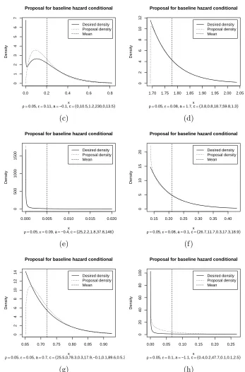
In the case, when the real distribution fλj(x) is exactly Gamma, the proposal
distribution is equal to it, otherwise they are hopefully close enough to each others.
The Figures 1a–1h illustrate how the proposal distribution is close to the
4. OBTAINING RANDOM SAMPLE FROM THE POSTERIOR DISTRIBUTION 25 and r0 = 5. The power Ej of the polynomial is chosen randomly from the Poisson
distribution, the constraint a is drawn from the normal distribution, and the
coeffi-cients cs are generated from gamma and then shifted by −a which ensures that all
cs ≥ −a. The scale parameter ε is calculated as ε = (c0+Rj1)∆tj with Rj generated
from Poisson distribution.
Figure 1. Comparing real and proposal distribution for sampling from
the full conditional of the baseline
0.8 0.9 1.0 1.1 1.2 1.3 1.4
0
1
2
3
4
5
6
Proposal for baseline hazard conditional
ρ =0.05, ε =0.14, a=0.8, c=(7.4,0,2.1) x
Density
Desired density Proposal density Mean
(a)
0.00 0.02 0.04 0.06 0.08
0
100
200
300
400
500
600
Proposal for baseline hazard conditional
ρ =0.05, ε =0.17, a=−1.8, c=(0.4,0.5,1) x
Density
Desired density Proposal density Mean
(b)
We see that proposal distribution follows the form of a desired distribution well.
The main feature to notice is that localization regions of both distributions are the
same, which is needed for good convergence of the MCMC algorithm. This shows us
that the proposals are satisfactory.
However, this method of finding the proposal distribution has one hidden
draw-back. The expansion of the polynomial P(x) = QEjs=1(x+cs) in (B.1.2) to the form
of PEjf=0dfxf requires the evaluation of 2Ej terms, so the computational complexity
4. OBTAINING RANDOM SAMPLE FROM THE POSTERIOR DISTRIBUTION 26
Figure 1. Continuation: Comparing real and proposal distribution
for sampling from the full conditional of the baseline
0.0 0.2 0.4 0.6 0.8
0 1 2 3 4 5 6 7
Proposal for baseline hazard conditional
ρ =0.05, ε =0.11, a=−0.1, xc=(0,10.5,1.2,230,0,13.5)
Density
Desired density Proposal density Mean
(c)
1.70 1.75 1.80 1.85 1.90 1.95 2.00 2.05
0 2 4 6 8 10 12
Proposal for baseline hazard conditional
ρ =0.05, ε =0.08, a=1.7, xc=(3.8,0.8,18.7,59.8,1.3)
Density
Desired density Proposal density Mean
(d)
0.000 0.005 0.010 0.015 0.020
0
500
1000
1500
Proposal for baseline hazard conditional
ρ =0.05, ε =0.09, a=−0.4x, c=(25,2.2,1.8,37.8,146)
Density
Desired density Proposal density Mean
(e)
0.15 0.20 0.25 0.30 0.35 0.40
0
5
10
15
20
Proposal for baseline hazard conditional
ρ =0.05, ε =0.08, a=0.1, cx=(26.7,11.7,0.3,17.3,18.9)
Density
Desired density Proposal density Mean
(f)
0.65 0.70 0.75 0.80 0.85 0.90
0 2 4 6 8 10 12 14
Proposal for baseline hazard conditional
ρ =0.05, ε =0.05, a=0.7, c=(25.5,0,78.3,0.3,17.9,−0.1,0.1,89.6,0.5,34.3x
Density
Desired density Proposal density Mean
(g)
0.00 0.05 0.10 0.15 0.20 0.25
0 20 40 60 80 100
Proposal for baseline hazard conditional
ρ =0.05, ε =0.1, a=−1.1, cx=(0.4,0.2,47.7,0.1,0.1,2.5)
Density
Desired density Proposal density Mean
4. OBTAINING RANDOM SAMPLE FROM THE POSTERIOR DISTRIBUTION 27 So, for the case of large Ej instead of direct expansion we recommend using the
following method. The coefficientd0 can be easily obtained by simple multiplication:
d0 =
Ej Y
s=1
cs, (2.4.6)
and the coefficient dEj is equal to 1. Regarding the rest Ej −1 coefficients, we can
evaluate the polynomial P(x) atEj −1 different points x1, . . . , xEj−1 and find these coefficients by solving the linear system of equations:
Ej−1
X
s=1
dsxs1 = P(x1)−x
Ej
1 −d0,
. . .
Ej−1
X
s=1
dsxsEj−1 = P(xEj−1)−x
Ej
Ej−1−d0.
(2.4.7)
Note that value x = 0 should not be used for any of the points xs to avoid the
presence of noninformative equation 0 = 0.
This method of polynomial expansion is much faster than the direct expansion
but suffers from numerical instability because of the presence of high powers of xs.
So for large Ej the precision provided by the default floating point variable type in
most of the mathematical packages and programming languages is not enough to
obtain satisfactorily precise values of ds. So one should use some non-standard types
providing higher precision. For the programming language C one can use the type
mpf twhich can be found in the GMP library or the type mpfr t which can be found
inMPFR library.
4.1.2. Finding the proposal distribution using the mode of the full conditional. An
4. OBTAINING RANDOM SAMPLE FROM THE POSTERIOR DISTRIBUTION 28 fλj(x) in the region x > max{a,0} and then derive the proposal distribution based
on such local maximum.
The proposition below allows us to find whether such local maximum exists and
when it does to find its region of localization.
Let cmin = min
1≤s≤Ejcs be the minimum of the coefficients cs of fλj(x) defined in
Proposition 4.1, andcmax = max
1≤s≤Ejcs be the maximum of them.
Also define the following two values (if the expressions under the square roots are
non-negative):
xL=
1 2
ε(ρ+Ej−1)−cmax+ q
(ε(ρ+Ej−1)−cmax)2+4ε(ρ−1)cmax
, (2.4.8)
xU=
1 2
ε(ρ+Ej−1)−cmin+ q
(ε(ρ+Ej−1)−cmin)2+4ε(ρ−1)cmin
. (2.4.9)
Proposition 4.3. The following statements for the greatest extremum xˆ of the
pdf fλj(x) in the region x >max{a,0} are true:
(1) If xU is undefined or xU ≤max{a,0} then fλj(x) does not have extrema for
x >max{a,0} and is strictly decreasing in this region.
(2) If there exist extrema of fλj(x) in x > max{a,0} then there are only finite
number of them and the greatest extremum, x, is a local maximum. In addi-ˆ
tion, in this case,xU is guaranteed to be defined and xˆsatisfies the inequality
max{a,0}<xˆ≤xU.
(3) If xL is defined and xL > max{a,0}, then both xˆ and xU are defined and
satisfy the inequality max{a,0}< xL ≤xˆ≤xU.
4. OBTAINING RANDOM SAMPLE FROM THE POSTERIOR DISTRIBUTION 29 Now, for the first case stated in Proposition 4.3, i.e. when xU is undefined or
xU ≤ max{a,0}, we set ˆx = max{a,0} as the maximum. Note that the value of
fλj(x) can be infinite at this point.
IfxU is defined andxU >max{a,0}, we are sure that if ˆxexists it satisfies ˆx≤xU.
So we can constrain the search for ˆxto the region max{a,0}< x≤xU.
Also, if the third condition is satisfied, i.e. xL is defined and xL>max{a,0}, the
region for the search can be constrained to the region xL≤x≤xU.
We use the modified Newton-Raphson optimization algorithm which searches for
extremum in an open interval. The details about this algorithm are presented in
Appendix C.
This algorithm attempts to find the extremum in the specified open interval (L, U)
and guarantees that the returned value belongs to this interval even if the desired
extremum is not found. The ability of the algorithm to return some well-defined value
of xfor any input is essential for our application. If we find any finite point ˆx in the
regionx >max{a,0}and construct the proposal distribution with the support in this
region and mode at ˆx, the MCMC algorithm will work with this proposal. However,
in order for the proposal distribution to be close to the desired full conditional, we
try to use not the arbitrary point but the maximum and only if we fail to do so we
rely on the fact that this point can be chosen arbitrarily.
We can run this algorithm with the limits L and U found as follows:
L =
(
max{xL, a,0}, if xL exists,
max{a,0}, otherwise, (2.4.10)
4. OBTAINING RANDOM SAMPLE FROM THE POSTERIOR DISTRIBUTION 30 Note that, if the maximum is reached at either L or U, the algorithm will not
return exactly this value but a value very close to it.
It is worth mentioning that even if the extremum does not exist, the algorithm
will still give some value between L and U. This means that if we do not succeed in
finding the largest extremum offλj(x) we still obtain some value of ˆx which can be
used for construction of the proposal distribution.
After we find the ˆx, we can use the Gamma proposal shifted by the value max{a,0}
as before, and we set the scale parameter of it equal to the scale parameter of the
original distribution ε = 1/((Rj +c0)∆tj). The shape parameter ν of the proposal
distribution is chosen such that the mode of this distribution is equal to ˆx. That is,
we set:
ν = xˆ−max{a,0}
ε + 1. (2.4.12)
Note that proposal distribution found by any of the two discussed methods is
not an approximation of the desired conditional distribution in any way but it only
follows the shape of this distribution. However, the shape similarity is enough for
our purposes, since wrapping the sampling from it into a Metropolis-Hastings step
adjusts for any differences in these distributions.
4.2. Sampling from the regression functions conditional distribution.
The distribution of the component of one regression function αkj conditional on all
4. OBTAINING RANDOM SAMPLE FROM THE POSTERIOR DISTRIBUTION 31 Let q be the number of individuals who had an event in the interval (tj−1, tj] and
whosek-th covariates were not zero at the moment of event. Also suppose that these
individuals have indicesi=i1, . . . , iq in the original dataset.
In addition, denote the constant
Cconstr = −λj −
X
k06=k
min
αk0jinf Ωk0, αk0jsup Ωk0
− min
1≤l≤nωlj !
, (2.4.13)
coefficients
cs =
1 zikj
λj + X
k06=k
αk0jzik0j +ωl
isj
!
, (2.4.14)
ε =
N X
i=1
Rijzikj !
∆tj, (2.4.15)
and the constraints
a=
(Cconstr
supΩk if supΩk >0,
−∞ otherwise,
b =
(Cconstr
infΩk if infΩk <0,
+∞ otherwise.
(2.4.16)
Proposition 4.4. The probability density function fαkj(x) of αkj conditional on
all other parameters is proportional to:
fαkj(x)∝ q Y
s=1
(x+cs) !
exp (−εx)I{a≤x≤b}, (2.4.17)
Proof. The proof is presented in Appendix B.
Similarly to the baseline hazard, we propose two methods of constructing the
proposal distribution
4.2.1. Construction of proposal distribution using the mean of the full conditional.
4. OBTAINING RANDOM SAMPLE FROM THE POSTERIOR DISTRIBUTION 32 Let df be the coefficients of the polynomial Pqf=0dfxf obtained by expansion of
the product Qqs=1(x+cs) in the pdf fαkj(x) defined in Proposition 4.4.
Now, if ε 6= 0 denote
I0 =
1 ε
exp(−εa)−exp(−εb)
, (2.4.18)
If =
1 ε
afexp(−εa)−bfexp(−εb) +fIf−1
, f = 1, . . . , q, (2.4.19)
where in case of infinitea orb the values of the corresponding functions are evaluated
as limits when argument approaches infinity.
In the case ε= 0 let
If =
bf+1−af+1
f+ 1 , f = 0, . . . , q, (2.4.20)
where we suppose thata and b are both finite.
Proposition 4.5. The normalizing constantCnorm and the meanµ of the
distri-butionfαkj(x) can be found as:
Cnorm = q X
f=0
dfIf, (2.4.21)
µ =
Pq
f=0dfIf+1
Pq
f=0dfIf
. (2.4.22)
Proof. The proof is presented in Appendix B
In the case of ε6= 0, we can use proposal of the form:
S+ sign(ε)G
ν, 1
|ε|
, (2.4.23)
whereS is equal toa orb depending on the sign of ε:
S =
(
a, if ε >0,
4. OBTAINING RANDOM SAMPLE FROM THE POSTERIOR DISTRIBUTION 33 and ν is calculated in a such way that the mean of the proposal distribution is equal
to the meanµ obtained earlier, i.e.:
ν=ε(µ−S). (2.4.25)
So the proposal density g(x) becomes:
g(x) = |ε|
ν
Γ(ν)
sign(ε)x−S
ν−1 exp
− |ε|(sign(ε)x−S)
. (2.4.26)
For ε = 0 we can use the Gaussian proposal with mean equal to µ and standard
deviation τ which provides the same ratio of Gaussian pdf g(x) at mean µ and one
more point y (the choice of which will be discussed later) as that of the original
distributionfαkj(x) at the same points:
g(µ) g(y) =
fαkj(µ)
fαkj(y)
⇔ 1
exp−(y2−κµ2)2
=
fαkj(µ)
fαkj(y)
⇔κ=
v u u t
(y−µ)2
2 lnffαkj(µ)
αkj(y)
. (2.4.27)
The point y is chosen to be 0.1µ+ 0.9a or 0.1µ+ 0.9b whichever produces the
greater value of fαkj(x). We do not use the points a and b since fαkj(x) can be 0 at
both of them.
4.2.2. Construction of proposal distribution using the mode of the full conditional.
Similarly to the proposal distribution of baseline hazard, we can construct the
pro-posals for regression functions without expanding the polynomial. Instead, we are
trying to find the mode of the distributionfαkj(x) and construct the proposal density
g(x) with the same mode.
The following proposition describes the possible behaviour of the function fαkj(x)
4. OBTAINING RANDOM SAMPLE FROM THE POSTERIOR DISTRIBUTION 34
Proposition 4.6. Provided that q and ε are not simultaneously equal to 0, the
density fαkj(x) satisfies one of the following conditions:
(1) fαkj(x) has a unique maximum in the region a < x < b.
(2) fαkj(x) is strictly decreasing in the interval a < x < b, in which case a is
finite.
(3) fαkj(x) is strictly increasing in the interval a < x < b, in which case b is
finite.
Moreover, if q 6= 0, the modified Newton-Raphson algorithm explained in
Appen-dix C applied to the functionfαkj(x)with the limits L=aandU =balways converges
to a finite value.
Proof. The proof is presented in Appendix B.
So in the case of q 6= 0, our modified Newton-Raphson algorithm will converge to
some satisfactory value, and in the case of q = 0, the maximum is ˆx =a if ε >0 or
ˆ
x=b if ε <0 and is always finite.
The obtained point ˆx can be used for construction of a proposal distribution.
We consider the same form of proposal distribution as in the previous section, i.e.
distribution given by formula (2.4.23) in the case of ε6= 0 and Gaussian proposal in
the case ofε= 0.
The shape parameter ν of the Gamma distribution can be found as ε(ˆx−S) + 1,
the scale parameter remains 1
4. OBTAINING RANDOM SAMPLE FROM THE POSTERIOR DISTRIBUTION 35 If ε = 0 we use the Gaussian proposal with mean at ˆx and standard deviation
found through the equality of ratios like before.
4.3. Sampling from the frailty’s full conditional distribution. The condi-tional distribution of the frailtyωlj given all other parameters is given by the following
proposition.
Let q be the number of individuals from the l-th region who had an event in the
interval (tj−1, tj]. Also suppose that these individuals have indices i = i1, . . . , iq in
the original dataset.
Let the limits a1 and b1 be
a1 = −λj − p X
k=1 min
αkjinf Ωk, αkjsup Ωk
, (2.4.28)
b1 = +∞, (2.4.29)
and the parameters µ0 and δ be
µ0 = θ2
j
ml
R(jl)∆tj+ωlj, (2.4.30)
δ2 = θ 2
j
ml
. (2.4.31)
Proposition 4.7. The density fωlj(x) of the parameter ωlj conditional on all
other parameters is proportional to:
fωlj(x)∝ q Y
s=1
(x+cs) !
1
√
2πδ2 exp
−(x−µ0)
2
2δ2
I{a1 < x < b1}. (2.4.32)
Proof. The proof is presented in Appendix B.
4.3.1. Construction of proposal distribution using the mean of full conditional.