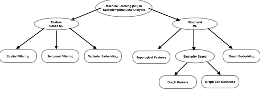
ABSTRACT
SENCAN, HUSEYIN. (Dis)Similarity-based Classification Of Cross Domain Multivariate Spatiotemporal Systems Using Dynamic Network Structures and Graph Edit Distances. (Under the direction of Dr. Chang S. Nam and Dr. Robert St. Amant.)
Many complex systems can be naturally represented as networks. Consider the human
brain, where coherent physiological activity among neural elements in spatially distant
brain locations creates cognitive functions; or climate, in which a grid of oscillators
gov-erns oceanic-atmospheric circulations; or finance, as a collection of stock markets; or
social interactions in general. In the literature, topological structures of such networks have been analyzed extensively.
From a statistical learning viewpoint, dynamic changes in these network structures
can be associated with events that emerge from the underlying structures. For instance,
dynamic changes in brain network structure may correspond to an inherent cognitive
dysfunction or a unique function. Changes in a climate network may correspond to a
natural phenomenon such as an extreme event like a hurricane or a drought. Structural
changes in a social network such as the science collaboration network may point to a
political paradigm shift.
The first part of this dissertation evaluates classification and inference methods for spatiotemporal datasets (subject to scope of this thesis) and identifies suitable approaches
for handling spatiotemporal patterns, as well as challenges and gaps in current learning
algorithms. These act as motivation for the current work. Further, possible future
direc-tions for the analysis of spatiotemporal data are identified.
The second part of this dissertation describes a graph-theoretic approach for the
classification of (extreme) events emerging from spatiotemporal physical systems based on
underlying network structures. A novel, efficient dissimilarity-based pattern classification
algorithm using the distances between network structures created from spatiotemporal
processes as input is proposed to predict the outcome of such events as an alternative to existing feature-based classification methods.
Finally, the dissertation presents motivating examples and application areas for which
the proposed methods are suitable, along with evaluation metrics that demonstrate their
validity and superiority to existing approaches. Four datasets from two distinct
problems and selected as target applications: (1) from the cognitive science domain,
predicting subjects’ mental states in two separate electroencephalogram (EEG)-based
cognitive science experiments, and (2) from the climate domain, forecasting landfall
be-havior of North Atlantic and South West Indian ocean hurricane trajectories. Results
show that network-based classification approaches for the target datasets outperform
© Copyright 2016 by Huseyin Sencan
(Dis)Similarity-based Classification Of Cross Domain Multivariate Spatiotemporal Systems Using Dynamic Network Structures and Graph Edit Distances
by
Huseyin Sencan
A dissertation submitted to the Graduate Faculty of North Carolina State University
in partial fulfillment of the requirements for the Degree of
Doctor of Philosophy
Computer Science
Raleigh, North Carolina
2016
APPROVED BY:
Dr. Matthias Stallmann Dr. Dennis R. Bahler
Dr. Chang S. Nam
Co-chair of Advisory Committee
BIOGRAPHY
Huseyin Sencan was born in Antalya, Turkey. After graduating from (Istanbul) Bogazici
University Computer Education and Technology Department with honors degree in 2004,
he continued his career as a Software Engineer for various industries. In 2006, he was
enrolled (Istanbul) Marmara University Computer Engineering Department from which
he received his M.Sc. degree in 2009. He started his Ph.D. in North Carolina State
Uni-versity Computer Science department in Fall 2009 and successfully defended his Written Preliminary in Fall 2012, then Oral Preliminary in Summer 2015 under the guidance of
Dr. Robert St. Amant and Dr. Chang S. Nam. During his Ph.D., he worked in various
research projects as a research assistant and application designer/developer; such as
be-tween 2012 and 2013 in ISE Brain-Computer Interface Laboratory, bebe-tween 2011 and
2012 in CSC Knowledge Discovery Laboratory, between 2009 to 2010 in CSC AI-Game
ACKNOWLEDGEMENTS
I would like to express my appreciation my co-advisors, Dr. Robert St. Amant and Dr.
Chang S. Nam for their guidance, support and patience throughout my research. I would
not be able to complete this work wither their help. I would also like to thank Dr. Matthias
Stallmann and Dr. Dennis R. Bahler for accepting to be member of my committee and for
their valuable comments and suggestions. I would also like to thank Dr. Michael Young,
and Dr. Nagiza Samatova whom I had a chance to work with in the beginning of my PhD here at NC State. In addition, many thanks to my friends and fellow graduate students
Can Babaoglu and Prairie Goodwin for their help and comments throughout my PhD.
Last but not least, I would also like to thank my family for their continuous support and
TABLE OF CONTENTS
List of Tables . . . vi
List of Figures . . . vii
Chapter 1 Introduction . . . 1
1.1 Problem Statement and Research Questions . . . 4
1.2 Thesis Statement . . . 5
1.3 Dissertation Contributions . . . 5
1.4 Dissertation Outline . . . 6
Chapter 2 Background Work . . . 7
2.1 Spatial Datasets and Classification . . . 8
2.2 Temporal (Time Series) Datasets and Classification . . . 10
2.3 Spatiotemporal Datasets and Classification . . . 11
2.3.1 Classification of Human Cognitive States using EEG . . . 13
2.3.2 Classification and Predictive Modeling in Climate . . . 16
2.4 Network-based Approaches . . . 19
2.4.1 Brain Networks . . . 20
2.4.2 Climate Networks . . . 26
Chapter 3 Proposed Method: Similarity-Based Classification of Spatiotem-poral Datasets using Networks . . . 29
3.1 Similarities Between Spatiotemporal Systems . . . 30
3.2 Similarities Between Networks . . . 31
3.3 Graph Matching . . . 33
3.3.1 Exact Graph Matching . . . 33
3.3.2 Inexact Graph Matching . . . 34
3.4 Network Classification using (Dis)Similarities . . . 37
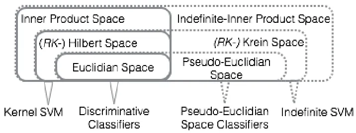
3.4.1 Learning with (indefinite-) Kernels and (pseudo-) Euclidian Space Embeddings of Dissimilarities . . . 39
3.4.2 Dissimilarity Space Embeddings . . . 45
3.4.3 (Nearest) Neighborhood-based Learning . . . 46
Chapter 4 Motivating Examples and Datasets . . . 47
4.1 Hurricane Track Classification . . . 47
4.1.1 Dataset I - Atlantic Ocean Hurricanes . . . 48
4.1.2 Dataset II- Indian Ocean Hurricanes . . . 48
4.1.3 Climate Data and Preprocessing . . . 49
4.2 Classification of Human Cognitive States . . . 50
4.2.2 Dataset IV - Mental Task Classification . . . 50
4.2.3 EEG Data and Preprocessing . . . 51
Chapter 5 Experimental Results and Discussion . . . 53
5.1 Classification Algorithms on Raw (Tabular) Data . . . 54
5.1.1 Support Vector Machines . . . 54
5.1.2 k-Nearest Neighbor Classifiers . . . 56
5.1.3 Decision Trees . . . 56
5.1.4 Naive Bayes . . . 57
5.1.5 Results . . . 58
5.2 Feature Selection Algorithms . . . 58
5.2.1 t-Score . . . 60
5.2.2 F-Score . . . 60
5.2.3 Information Gain . . . 60
5.2.4 Minimum redundancy, maximum relevance . . . 60
5.2.5 Fast Correlation-Based Filter . . . 61
5.2.6 CFS . . . 61
5.2.7 Results . . . 61
5.3 Dimensionality Reduction, Feature Extraction and Domain Specific Features . . . 64
5.3.1 Principal Component Analysis . . . 65
5.3.2 Common Spatial Patterns . . . 65
5.3.3 Climate Indices . . . 65
5.3.4 Correlations / Coherences as Features . . . 66
5.3.5 Results . . . 67
5.4 Similarity-Based Classification . . . 70
5.4.1 Similarities across components of spatiotemporal systems . . . 71
5.4.2 Structural Similarities Between Networks and Classification . . . 71
5.4.3 Spectral Features . . . 74
5.4.4 Multi-dimensional Scaling . . . 76
5.4.5 Converting Distances into Similarities . . . 76
5.5 Comparison of Feature and Similarity-based Approaches . . . 79
Chapter 6 Conclusions . . . 81
6.1 Contributions to Computer Science . . . 82
6.2 Contributions to Cognitive Science . . . 84
6.3 Contributions to Climate Science . . . 85
6.4 Limitations . . . 85
6.5 Future Work . . . 87
LIST OF TABLES
Table 5.1 Overall cross validation accuracies for tabularly embedded data for each classification algorithms. Highest and significantly improved statistics are displayed in bold. . . 58 Table 5.2 Cross validation accuracies for filter and embedded feature selection
algo-rithms across all four benchmark datasets. Highest and significantly im-proved statistics are displayed in bold. . . 62 Table 5.3 Cross validation accuracies for specific feature selection algorithms across
four benchmark datasets. Highest and significantly improved statistics are displayed in bold. Climate indices are domain specific features for climate data. CSP as a supervised feature selection technique developed for brain EEG is also applied in climate data. PCA is a generic dimensionality re-duction technique. Correlations between times series in climate data, and coherences in EEG data are implemented as problem/domain specific features. 66 Table 5.4 Cross validation accuracies for similarity-based learning algorithms using
temporal similarities across spatiotemporal systems. . . 71 Table 5.5 Cross validation accuracies for classifiers using spectral graph features
ex-tracted from each network separately, and multi-dimensional scaling embed-dings of graph edit distances. Highest and significantly improved statistics are displayed in bold. . . 72 Table 5.6 Cross validation accuracies for (dis)similarity-based classification of graph
edit distances after transformed into similarities through four different (S1,
S2, S3,S4) linear and nonlinear transformation functions as listed in
LIST OF FIGURES
Figure 2.1 Overview of classification methods for spatiotemporal data. . . 8 Figure 2.2 Vectorial embedding of three-dimensional spatiotemporal data into
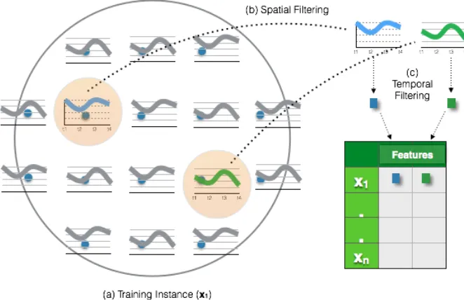
two-dimensional tabular format for the purpose of canonical data classification. 11 Figure 2.3 Machine Learning Framework - Intertwined, three-step process:
preprocess-ing, feature selection, and classification or regression. . . 13 Figure 2.4 Spatial and temporal filtering of spatiotemporal process (a) data is
repre-sented as it is acquired, (b) spatial locations that are making a difference in classification are selected, (c) time series data is filtered and summarized in a single point using temporal filtering techniques.. . . 15
Figure 3.1 Similarities between spatiotemporal processes: (a) first pairwise similarities at each spatial locationsi ∈S are calculated separately between all sample
(training) instances inX, (b) calculated similarities for each spatial location
siare represented as a separate similarity matrixKi, then (c) using a
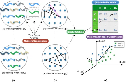
combi-nation function (f) an aggregated similarity matrix is calculated and given, along with the corresponding class labels for each row, to a similarity-based classifier to build a classification model. . . 30 Figure 3.2 Method overview for the proposed network-based classification framework:
(a) each event with an outcome yi is associated with a spatiotemporal
pro-cess (xi), (b) networks are generated based on the statistical correlations/
coherences between time series, (c) the distances between pairwise network instances are computed using graph matching techniques and the resulting distance matrix (D) used as input to dissimilarity-based classifiers. . . 32 Figure 3.3 Example 1 - edge distance calculation, spatial networks with a single edge. 36 Figure 3.4 Example 2 - edge distance calculation, spatial networks with multiple edges. 37 Figure 3.5 Metric and non-metric spaces and corresponding learning algorithms. . . . 39 Figure 3.6 Flowchart of the classification algorithms using dissimilarities (D) -
embed-ded and kernel-based classification methods. . . 41 Figure 3.7 Classiifcation using D as kernel, (a) dissimilarities are converted into
sim-ilarities, then classified using (indefinite-) kernel-based approaches (b) dis-similarities are embedded into (pseudo-) Euclidian spaces then classified using vector-based classifiers. . . 44 Figure 3.8 Dissimiarity space embedding and classification (a) during training, a set
of graphs are selected as part of the prototype set selection step, (b) testing instances are embedded agains this. . . 45
Figure 4.2 Motivating Example II - Mental Transformation Task. First subject’s base-line signal is recorded, then a mental transformation task in 2d appears on the screen for 15secs, in the final screen, the subject is asked to choose matching object in 3d with the projected view. . . 51
Figure 5.1 Decision boundary for linear Support Vector Machines. . . 55 Figure 5.2 Decision boundary for nonlinear (kernel) Support Vector Machines. . . 56 Figure 5.3 Decision boundaries for filter-based feature selection algorithms over
cog-nition dataset; xy coordinates represent features with the highest weights as a result of CFS feature selection. Local classifiers in (a) and (b) overfit the data in order to reduce the training error. Model-based parametric (c), linear (d), (e) and non-linear global classifiers (f)-(h) fit more generalizable decision boundaries but could not separate the data into two classes. . . . 63 Figure 5.4 Decision boundaries for domain-specific (coherence) features on cognition
dataset;xycoordinates represent coherence features with the highest weights as a result of CFS feature selection applied for visualization purposes. As local classifiers kNN (a) divides the space into local neighborhood regions, decision trees (b) divide the space into local rectangles. Parametric Naive Bayes (c) distinguish the data based on class distributions. Linear (d), (e), and nonlinear kernel classifiers (f)-(h) fit a global model on the data. . . . 68 Figure 5.5 Performance comparison of local vs model-based classifiers on cognition
data using coherences as features. On the left, the accuracies are shown when the same subject’s data is not allowed to be in both training and testing sets (heterogeneous data) at the same time, and on the right, random sampling where the test data is randomly selected among all instances and the data from the same user is allowed to be in both training and testing sets. . . 69 Figure 5.6 Decision boundaries for spectral features on the cognition dataset; xy
co-ordinates represent eigenvalues corresponding to largest eigenvectors. The data is scattered in two dimensions. Local classifiers in (a) and (b) overfits the data in local regions, parametric (c) and model-based linear classifiers (d), (e) fit a global model to enable generalization. Nonlinear kernel-based classifiers in (f)-(h) create nonlinear decision boundaries for the data. . . 73 Figure 5.7 Classification decision boundaries for MDS embeddings; the coordinate
Figure 5.8 Similarity matrix representation for each sample dataset, similarities be-tween instances acquired from (a) Cognition dataset, (b) Atlantic Ocean hurricanes, (c) Indian Ocean hurricanes, and (d) Graz-BCI experiment data. 78 Figure 5.9 Comparison of overall classification (SVM) accuracies of feature and
similarity-based classifiers for each dataset. The average accuracies across all datasets are listed in the last column. . . 79 Figure 5.10 Statistical analysis of the results; (a) Kruskal Wallis test results: the mean
Chapter 1
Introduction
Analyzing dynamical systems from a physics point of view requires extensive amounts
of information about system dynamics, such as the interactions between particles at a
micro or reduced macro scale. Ideally, a dynamical system can be described by a set of
differential equations [89]. However, some systems are too complicated to be described
exactly, and some are not subject to such a reduction due to insufficient knowledge. In the literature, these are referred to as complex systems [52]. Typical examples of
complex systems are (1) the human brain, where the cognitive functions such as learning
or memory are outcomes of the dynamic interactions between distant neuron groups, and
(2) climate, in which atmospheric, geographic and biological factors contribute to the
changes in a nearly chaotic system. These two domains are the focus of this dissertation.
Data-driven statistical models that predict events by learning relationships with
ob-served or simulated variables have had a significant impact on our lives, due to their
success in many disciplines of science over the last several decades, in physics but also
in a wide range of other domains [109]. With the increase of available data, accessible
computational power, and the development of robust statistical models, we have seen a rapid transition in the treatment of problems that were formerly viewed as
impracti-cal to solve. As might be expected, data-driven models are also gaining ground in the
analysis of complex systems, as an alternative or a complementary approach to current
physics-based simulations.
Methods used in data-driven statistical analysis traditionally depend on the
assump-tion that adjacent observaassump-tions are independent and identically distributed. However,
true. For instance, climate scientists collect oceanic and atmospheric data over a region
from equidistant locations in predetermined time intervals, either by direct observation
or using sensor satellite images. Economists constantly record daily stock market
quo-tations to be able to follow the trends in financial markets. Brain imaging uses mapped
electrodes attached to the subject’s scalp in order to collect signals with a fixed sample
rate in a variable length experiment sessions. All of these datasets, constructed from
complex systems, intrinsically have high auto-correlation and dependency between
sys-tem variables. The syssys-tematic approach that aims to answer mathematical and statistical
questions posed by these spatial and temporal correlations has its own unique branch in
statistics and commonly referred to as spatiotemporal data analysis [102]. The first part of this dissertation explores a particular branch of spatiotemporal data mining, inference
analysis in spatially and temporally extended dynamical systems.
Inference algorithms, in particular classification methods independent of the
repre-sentation of the data they operate on (i.e., structured or tabular data), try to automate
the classification process using a learned model built upon a sample prototype set;
intu-itively, such algorithms are comparable in some ways to our human ability to recognize
general patterns by looking at examples. In this respect, the majority of general purpose
classification algorithms start with a model generation step using a representative data
called a training set in a particular domain. The goal for the learned model is to be able to generalize well to unseen real world examples contained in a test set. For instance,
if the learning algorithm is designed to distinguish humans from the cars in a traffic
video surveillance application, then we need a sample set of representations of cars and
humans in our training algorithm, taken from existing footage. Then a model can utilize
the derived characteristics or features of both classes to create a set of rules and
equa-tions, or it can look for specific templates to match; which approach is taken depends on
the selected learning methodology and representation. In this respect, depending on the
representation of objects in the example domain, the learning algorithms can be designed
in two distinct ways: statistical and structural.
In the statistical approach, the model can be constructed either from the tabular
raw data or from a set of features generated or selected from the raw data. (Feature
generation and selection methods are also two distinct paradigms under the statistical
machine learning framework and will be discussed in detail in later chapters.) In the car
and so forth of each object can be declared as features and listed in tabular numerical
form. Together, these form a feature (vector) space where each instance of the data can be
represented as a point inn dimensional Euclidian space. The calculated metric distances between these vectors feed a learning algorithm, in which the goal is to optimize the model
by minimizing the targeted error function. Metric operations such as transformations,
inner products, and defined norms that preserve the underlying Euclidian geometry give
us a rich set of mathematical tools, resulting in a well established statistical learning
theory. Nevertheless learning is inherently restricted to the generated/selected
feature-vector space; it is therefore limited in terms of discovering possible structural relations
between training instances.
Structural pattern recognition, on the other hand, mines the data in order to find
primitives, definitive and relational substructures. Structural methods have been found
most effective in domains in which inherent natural structure exists, such as molecular
and protein datasets, hand writing recognition, fingerprint, and network classification
problems [3, 46, 73]. In chemical compound classification, for instance, the existence or
lack of a particular molecule within a structure may tell us whether a given chemical
is part of a toxic family or not. Thus, in structural learning algorithms, features can be
defined as substructures, primitives, motives, or communities, and the presence or absence
of these features in a new sample determines the target class of that instance. However, the drawback of a discriminative motive searching approach is that learning is tied to
binary-valued features. The lack of mathematical framework in decision making limits
the broad use of structural learning algorithms in classification, despite their intuitive
nature.
One of the main theories about human learning suggests that we learn from
exam-ples and that we differentiate things by looking at differences between objects, even if
such differences are not explicitly defined in advance as features. This is in contrast to
conventional statistical machine learning algorithms, which are designed to work with
existing features [29]. For example, given an object, we can classify and label it based on how similar the object is to some reference point. This approach to considering implicit
structural features leads to the formation of a class of hybrid learning methodologies
called similarity- or dissimilarity-based pattern recognition algorithms, which typically
utilize evolutionary learning principles to form a class description by stating thata class
(dis)similarity-based classification algorithm can be constructed without the need for
pre-processing to extract or generate artificial features. In this respect, dissimilarity-based
classification does two things; it combines the representative power of the structural
and solid mathematical framework of statistical learning algorithms using the notions
of proximity and dissimilarity space, and it eliminates the need for cumbersome feature
generation or primitive substructure searching processes to a great extent.
In the second part of this dissertation, we explain the use of (dis)similarity-based
classification algorithms to analyze complex network structures generated from domain
independent spatiotemporal datasets using graph edit distance measures.
1.1
Problem Statement and Research Questions
A spatiotemporal process x with an outcome y occurring over a set of spatial locations and within a certain time period can be represented as
y←x(s,t) :s∈Sandt∈T,
where T is the time interval in which the process occurs and S is the set of locations. If the goal is to predict the outcome of a future process ˆy, then using machine learn-ing algorithms is the natural choice. However, the majority of modern machine learnlearn-ing
algorithms are designed to work on tabular datasets where the inputs are composed of
features x ={x1, x2, ..xN}, with each (xi) representing unique and independent
charac-teristics of the data. The first research question is this: What techniques can be applied
to fit spatiotemporal data into an existing standard machine learning framework, or what
other alternative classification approaches can be utilized to predict the output of a
spa-tiotemporal process (within the scope of this thesis)?
With advances in network theory, many complex systems are now being represented
as networks. For example, the global climate system is represented by a grid of oscillators varying in some complex way [107]; the interactions between brain regions during task
execution are represented as functional brain networks [13]. Recently, these networks
have been analyzed with the goal of performing inference on them. The second research
question is this: Can we use these network structures for the purpose of classification of
events emerging from spatiotemporal processes instead of (or complementary to)
feature-based approaches? Additionally, what are other possible techniques that we can utilize to
1.2
Thesis Statement
To answer the first question, we explore existing features and feature-based classification
approaches in each domain (i.e. climate and cognitive science). Since the domains share
similar spatiotemporal characteristics, we list the approaches that can be transferable
from one domain to another and give an overview of methods to create a framework for
common learning approaches. We show that spatiotemporal processes can be embedded
into the standard machine learning framework by utilizing a set of spatial and temporal filtering techniques.
For the second research question, our hypothesis is that for inference in complex
phys-ical systems, network-based classification, where the interactions between distant spatial
locations are the determining factor for overall system behavior, is a valid alternative
to existing data mining algorithms for predicting emerging event characteristics. We
also add that, for classification of spatial networks, (dis)similarity-based learning, using
the proposed graph edit distance formulation, contributes to a more effective structural
learning strategy compared to existing (spectral) graph embedding techniques.
1.3
Dissertation Contributions
The overall contributions of this research can be summarized as follows:
1. A unified framework has been created for classification in complex systems exhibit-ing spatiotemporal characteristics. Suitable and non-suitable approaches, challenges and
gaps in the existing learning algorithms designed for classification in such systems have
been identifed.
2.Two distinct real-world emergent phenomena have been formulated as spatiotemporal (network) classification problems: (1) from the domain of cognitive science, specifically
brain-computer interfaces (BCI), predicting cognitive state or expertise level of
experi-ment subjects during task execution, and (2) from the climate domain, forecasting landfall
behavior of hurricane trajectories.
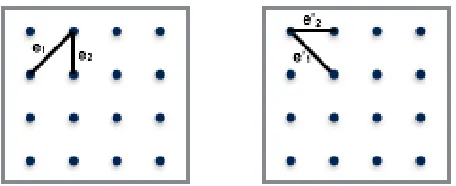
of the edges in a network structure is introduced, and in the second step, using the
ma-trix of matching costs, graph edit distance between network pairs is formulated as an
assignment problem.
4. It has been demonstrated that the graph-edit-based network classification approach outperforms existing machine learning techniques on problems in the two real-world
spa-tiotemporal domains given above.
5. A detailed explanation of (dis)similarity-based learning approaches has been carried out, starting from arbitrary similarity or distance scores between instances in a proto-type set, then following with directions for classification of those objects in a projected
mathematical space. Each method has been analyzed to find suitable learning strategies
for classification of spatial networks.
1.4
Dissertation Outline
The remainder of this document is structured as follows. Chapter 2 reviews existing
re-search on spatiotemporal data classification. The methodology for network-based classi-fication of such data is explained in Chapter 3, where an introduction to
(dis)similarity-based learning approaches and corresponding space topologies is given. In Chapter 4,
motivating examples and experiment datasets from two distinct spatiotemporal systems,
brain-computer interfaces and climate, are introduced. Afterwards, evaluation metrics
Chapter 2
Background Work
The first two sections in this chapter cover classification in spatial datasets and
classi-fication in temporal datasets, respectively. The third section is more extensive: it first
describes feature-based approaches to classification in two domains, brain-related research
and climate research; it then turns to network-based analysis of the same domains.
In Figure 2.1, a general framework for spatiotemporal classification in scientific datasets is given. Though the branches in Figure 2.1 represent existing approaches in the climate
and cognitive science domains, the framework can be extended to any scientific data
clas-sification tasks for data that has both spatial and temporal dimensions. In the following
sections each branch of the framework tree will be discussed through the example studies
from both climate and cognitive science literature.
The majority of modern machine learning algorithms are designed to work on standard
relational datasets where the inputs are composed of attributes, each ideally
represent-ing unique and independent characteristics of the data. As a general convention these
attributes are called featuresand the algorithms utilizing those in learning referred to as
feature-based statistical learning algorithms.
A well known example for feature-based classification on relational data is the IRIS
dataset, where the features are the sepal and petal length and width information for three
flower types [4]. The IRIS dataset is small and simple; for more complex datasets that may
include higher dimensional features, another step, called feature selection or generation,
might be required to filter out less informative attributes. A detailed overview of feature
selection and projection methods for general purpose statistical learning algorithms can
Figure 2.1: Overview of classification methods for spatiotemporal data.
However, not all datasets are required to have independent and identically distributed
discriminating feature sets listed in their respective dimensions. Many real-world datasets, especially scientific datasets, are recorded continuously in at least one of the space and
time dimensions. Therefore adjacent recordings have dependency on each other; this is
referred to as autocorrelation. In the analysis of spatiotemporal data, autocorrelation
needs to be taken into consideration to account for the characteristics of the data and to
produce objective results and meaningful analysis.
2.1
Spatial Datasets and Classification
Spatial data models using suitable geometric representations like points, lines, shapes
and images define the properties of static objects in space. Environmental and ecological
modeling using remote sensing satellite observations, geographic information systems
(GIS), telecommunication and mobility applications utilizing GPS locations are
well-known sources of vast amounts of spatial data. The increase in information resources and
application areas has triggered the demand for effective machine learning algorithms for
such data [99, 14].
For this reason, existing learning algorithms have been adapted for the analysis of
spatial data. Khan et al. [61] use a modified version of the kNN (k-nearest neighbors) classification algorithm with a set of metric distances calculated between spatial images,
spa-tially distributed features sequenspa-tially in tabular form is another way to employ existing
learning algorithms with such data. When it comes to the analysis of spatial features,
however, overlooking autocorrelation that exists between training instances may cause
poor inferences about the system being analyzed.
On the other hand, by incorporating spatial information into learning algorithms,
more suitable and effective tools can be created for the analysis of spatial data [99].
Markov random fields (MRF) applied in image segmentation problems and spatial
au-toregression (SAR) models used in regional economy and ecological data applications are
two examples of proven, successful implementation of spatial learning algorithms.
In SAR, the general logistic regression equation (Eq. 3.3),
y=Xβ+, (2.1)
is modified using the spatial contiguity matrix W and spatial dependency coefficient p (Eq. 2.2),
y =ρW y+Xβ+. (2.2)
The correction terms p, W and y introduced into the regression equation aim to remove systematic variations in the input dataX and in the residual error functiondue to spatial neighborhood relations.
A Markov random field-based Bayesian classifier is a model applied to image
segmen-tation and land-use classification problems. Experience with such models suggests the
importance of a spatial variable conditioned on the events only in its direct
neighbor-hood.
In classification using Naive Bayes, the probability that a given instance X belongs to a class ci can be computed from the conditional probabilities existing in the data
(Eq. 2.3):
P(ci|X) =
P(X|ci)P(ci)
P(X) . (2.3)
MRF modifies this formula by incorporating the neighborhood class label function L to estimate the posterior probability of a point belonging to class ci in the presence of
P(ci|X, L) =
P(X|ci, L)P(ci|L)
P(X) . (2.4)
2.2
Temporal (Time Series) Datasets and
Classifica-tion
Temporal data, also referred to as time series data, captures changes in a variable over a
time intervalT. The analysis of temporal data is studied extensively in statistics because of diverse resources in data and needs in application areas [101]. Sensors recordings of
the human body for cardiovascular activity monitoring, safety measurements of a nuclear
power plant, daily stock market values on Wall Street, and periodic sales numbers in a
company are just few examples of time series data.
As in spatial analysis, time series classification also faces challenges due to the nature
of the data. The characteristics of time series data include high dimensionality, temporal
autocorrelation, noise, nonlinearity and nonstationarity [2]. Learning algorithms working
in this domain needs to account for these challenges.
In general, time series classification algorithms are divided into three categories: feature-based, distance-based and model-based algorithms [33, 113].
The first approach preprocesses the data to generate a set of features, typically by
utilizing domain or expert knowledge. Generic machine learning algorithms that perform
well on standard datasets can also be used in feature-based time series classification
tasks [120].
The second approach frequently employed in sequential data classification is to
com-pute pairwise distances, which can either be standard (i.e. metric, such as Euclidian
distance) or non-standard (i.e. non-metric, as in dynamic time warping [62]), between
time series [9]. The calculated distances are given as input to a neighborhood-based clas-sification algorithm. Although this approach has been criticized for being primitive since
it does not involve any model building, it stands as an effective learning strategy in
classification.
As a third approach, model-based learning algorithms are employed in classification of
time series data. Hidden Markov Models and Neural Networks are promising for dealing
with intrinsic challenges introduced by temporal data since they cope with the temporal
Figure 2.2: Vectorial embedding of three-dimensional spatiotemporal data into two-dimensional tabular format for the purpose of canonical data classification.
are more sophisticated compared to feature and distance-based algorithms, requiring
in-depth analysis of the selected parameters prior to model building [66].
2.3
Spatiotemporal Datasets and Classification
In spatiotemporal datasets, variables extend in both spatial and temporal dimensions.
Datasets originating from ecological and environmental dynamics, climate, social and
daily interactions like transportation and traffic, physiological recordings of human body
and brain such as functional magnetic resonance imaging (fMRI), electroencephalogram (EEG) and magnetoencephalography (MEG) are all examples having spatiotemporal
characteristics. Despite advances in recording technologies and the emergence of new
application areas, a general framework is lacking for spatiotemporal data classification
methodologies in the current literature. One of the aims of this work is to draw a general
picture of machine learning algorithms for spatiotemporal systems.
Machine learning in general is an intertwined, three-step process: preprocessing,
fea-ture selection, and classification, as picfea-tured in Figure 2.3. Depending on the first two
steps, the nature of the data may change, and therefore the type of classification
preprocessed into noise-free data, so that a more complex algorithm can be employed
without fear of overfitting. If the high dimensionality of input data is reduced using a
feature selection algorithm, then a less robust, fuzzy classification algorithm can be
em-ployed. Selection of a classification method therefore depends on how the data is being
processed and which features are extracted from it. This may explain the reason for the
lack of a general framework for classification in spatiotemporal analysis, since
domain-dependent preprocessing and feature selection is determining factor for selection of a
classification approach.
A common but usually inefficient approach to any type of spatiotemporal system is
to reorganize each instance of data into a one-dimensional vector representation called a vectorial embedding, as shown in Figure 2.2. Mourao et al. [78] applied vectorial
embed-ding to fMRI data recorded in discrete time intervals at separate marker locations and
fed the resultant data to a Support Vector Machine classifier as input to create
classifi-cation model. The model discriminates between recordings of people assigned to perform
a cognitive task from people in resting state. The algorithm is named “Spatial-Temporal
SVM.” This is slightly misleading, because the algorithm does not incorporate any spatial
or temporal information such as autocorrelation into its model-building step. The results
of their study do not show any significant improvement over the comparison method
that uses features generated by taking the mean values across temporal dimension. The usefulness of vectorial embedding in analysis of spatiotemporal data has not yet been
proven.
Another commonly applied strategy for spatiotemporal data classification is to filter
out one or both of the space and time dimensions of the input. This can be done by
averaging over the temporal dimension, or by transforming time series data into more
compact forms such as spectral coefficients, or by selecting fewer spatial locations as
representative features. These examples of temporal and spatial filtering techniques are
illustrated in Figure 2.4. However, these transformations are application dependent and
requires domain knowledge in order to apply safely. In the reminder of this section, representative techniques for classification of spatiotemporal datasets contributing to this
research will be investigated within their respective domains. Each section begins with
a brief introduction to important classification problems in the domain, then continues
Figure 2.3: Machine Learning Framework - Intertwined, three-step process: preprocessing, feature selection, and classification or regression.
2.3.1
Classification of Human Cognitive States using EEG
Cognitive state classification is an important application area for brain-related researchand has many application areas. Designing brain computer interfaces, creating feedback
loops for advance training systems such as driving and flight simulators, allowing disease
diagnosis and prevention are just a few examples.
The data mining problems addressed by EEG-based cognitive science studies include
sequential pattern mining (to deal with extracting repetitive patterns from data such as
eye or muscle movements), associating relations of these patterns with cognitive brain functions [60], and outlier detection for differentiating abnormal brain states from normal
brain functions (such as epileptic seizures [35, 50] or schizophrenia [67]). In this research,
we focus on inference analysis (i.e. classification algorithms) for EEG-based cognitive
architectures.
Extraction of human cognitive states for the purpose of the above-mentioned
cations requires experiments conducted under laboratory conditions. While some
appli-cations collect data from subjects for diagnosis purposes in everyday non-laboratory
set-tings, others follow experimental procedures known as the synchronous and asynchronous
paradigms.
In asynchronous systems, a subject makes self-paced decisions to switch between available cognitive actions. The system is designed to capture and act according to these
mental changes. In the more common synchronous systems, experiments are divided into
fixed duration blocks called epochs. Each epoch is associated with the targeted task being
performed. For instance, a task might be to imagine oneself moving to the left or to the
right; each decision interval is associated with a clue shown to the subject on a computer
screen. From the EEG data recorded, a system tries to differentiate between the two
intended directions.
The input signal generated by those processes is an example of three-dimensional
fixed time interval T.
Feature Selection for BCI Datasets
The goal of feature selection in machine learning is to find a small subset of attributes
that sufficiently represents a larger set. However, in some types of data, including EEG,
such information is spread across all the dimensions of the input; therefore finding such a
subset may not be possible using standard feature selection techniques based on
statisti-cal correlations. Handling feature selection in each dimension (i.e. spatial and temporal) separately and introducing an intermediate step (i.e. feature identification) carried by
subject experts to account domain-specific characteristics is a common strategy applied
for this type of data.
Temporal Filtering
One of the fundamental theories about the electrical activity of the brain [6] suggests
that our brain rhythms change in accordance with the cognitive operation the brain
per-forms. For instance, during the resting awake state, the brain follows a posterior basic
rhythm called alpha modulation (7-14 Hz). During (imaginary) motor movements, the beta rhythm (15-30 Hz) is attenuated. Cognitive functions, on the other hand, activate
higher frequency gamma waves (30-100 Hz). These modulatory characteristics of the
sig-nal allow for identification of frequency domain features in EEG-based systems, because
frequency conveys information about the rhythmic activity of the brain during task
exe-cution. As a side effect, identification of this spectral component rules out the temporal
dimension of the input signal by summarizing the data collected over a course of time in
a single amplitude value.
Spatial Filtering
In addition to frequency domain transformations, spatial filtering is another common
technique for feature selection in EEG data. The goal of any spatial filtering is to
deter-mine an N dimensional unmixing matrix W weighted towards more important spatial components. When this matrix is applied to input signal x the result is a new signal y with emphasis on more discriminating channels (Eq. 2.5).
Figure 2.4: Spatial and temporal filtering of spatiotemporal process (a) data is represented as it is acquired, (b) spatial locations that are making a difference in classification are selected, (c) time series data is filtered and summarized in a single point using temporal filtering techniques.
A commonly used spatial filtering technique in the EEG domain is independent
com-ponent analysis (ICA), in which linear projections of the signal are computed to generate
statistically independent components [7]. In ICA, for N-channel EEG data, unmixing matrix W consists of N rows, each of which corresponds to an independent component in the signal. Selecting the first M of these N rows will reduce the dimension of the input signal by a factor of (1− N
M). In many applications, ICA is simply used for artifact
removal, due to its success in separating eye blinks and muscle movements from the raw
signal; therefore spatial filtering part is mostly achieved by its supervised successor, the Common Spatial Patterns (CSP) algorithm.
CSP is a supervised spatial filtering technique proven to be effective in a
num-ber of EEG-based brain computer interface applications in comparison to previous
ap-proaches [12]. The underlying principle of CSP is to maximize the variances between
signals that belong to separate classes via simultaneous diagonalization of the signal
co-variance matrices. The first and last entries of the resulting projection matrix W, sorted in descending order of the eigenvalues, explain the channels with largest variance and
Inference in EEG-based Systems
Although the spatial and temporal feature selection methods explained above can be
used as standalone techniques, they are usually applied in combination with each other.
For instance, frequency transformations can be performed after selection of discriminating
spatial channels. However, the ultimate success of the learning algorithms depends on the
selection of the right classification strategy. Lotte et al. [70] groups classification methods in machine learning domain according to their distinct characteristics: generative versus
discriminative, static versus dynamic, stable, and regularized algorithms. Since EEG
data is noisy and contain outliers, the regularization that minimizes the effect of outliers
and limits the unnecessary complexity of the model is stated as a required component
for this type of data. Nevertheless, researchers have tried a majority of the
state-of-the-art classification techniques with different feature selection strategies for EEG data.
Among others, Support Vector Machiness (SVM) are repeatedly reported as a suitable
and successful approach [79] due to SVM’s regulatory and generalizable characteristics.
In addition to SVM, dynamic classifiers such as Hidden Markov Models (HMM) is also reported as an effective technique for the current domain by Obermaier et al. [85],
because of their ability to cope with temporal aspect of the data inside the model.
2.3.2
Classification and Predictive Modeling in Climate
Climate is a system governed by physical, chemical and biological principles; the behavior
of the system can be approximately predicted using set of differential equations known
as model simulations. The complexity, resolution, initial conditions, variables and
pro-cesses included in a model result in different simulations whose predictions about the
distant and close future may vary marginally. One solution for the margin of error
prob-lem is averaging the simulation outputs to make commonsense predictions from model
ensembles [103].
While model simulations base their predictions on a set of initial conditions which requires limited data to build upon, the size of climate data is actually enormous and
growing exponentially. Remote sensor satellite images and output of model simulations
such as reanalyses [54], in which all the available but noisy heterogeneous observational
data is put through numerical simulations to generate large scale homogeneous datasets,
data-driven analysis of climate as an alternative or complementary approach for physics-based
simulations. However, the nature of climate data is spatiotemporal and there is a gap in
learning algorithms in data mining and machine learning to account for challenges such
as high dimensionality and auto- and cross correlation between input variables.
Active research problems in climate domain are grouped into four main categories by
Faghmous and Kumar in their recent study [32]: outlier and event detection, relationship
mining, pattern mining, and predictive modeling. In outlier detection the goal is to model
and differentiate anomalous events from the data such as the ones that have drastic effects
on the ecology like significant land cover changes [56], droughts or abnormal temperature
shifts [72].
Pattern mining tries to find motives or data clusters that share similar structure and
exhibit similar behavior that could also give greater insights about the rest of the data.
Pattern mining approaches in the climate field are applied to discover the dominant
signal in the high dimensional data via empirical orthogonal function (EOF) [5] and
Independent Component Analysis (ICA) [75] to find clusters exhibiting similar behavior
such as spatiotemporal neighborhoods. An interesting study is on finding hurricane track
patterns and identifying their characteristics across each distinct class of hurricanes [81].
Finding oceanic eddies is another open research problem because of their importance
in carrying information across oceans and forming teleconnections among geographic regions [32].
Relationship mining applications seek out relationships between some variables and
target events. For example, researchers have attempted to find correlations between sea
surface temperatures and global land surface temperature values [58] and fire patterns
in the Amazon [16] They have also related vertical wind shear in the Atlantic Ocean
to rainfall patterns in the African Sahel region [39]. Kim et al. [62] applied composite
analysis to relate five years hurricane data to warming patterns of the Pacific. McCloskey
et al. [74] take a different approach and relate Bermuda high pressure values to the curving
patterns of Cape Verde hurricanes.
These applications focus on explanations of phenomena. In predictive modeling, on
the other hand, given a set of data forming a process the goal is to create a model for the
process and to find the output of future processes by looking at the data. Machine learning
techniques are common in predictive modeling, such as in classification, by assigning the
learned equation. In the next subsections, the components of predictive modeling, feature
selection and learning algorithms applied for climate data will be covered.
Variable and Feature Selection for Climate Data
For climate, spatiotemporal variables such as daily sea level pressures (SLP), sea surface
temperatures (SST), vertical wind shear (VWS) and numerous other variables are
con-tinuously recorded by sensors (i.e. in situ and by satellite) and assimilated into model
simulations by major climatology institutions like NCAR-NCEP [37] and NASA [38]. Data-driven predictive models utilize these variables either by directly incorporating
them into their analysis [19], filtering relevant ones using statistical feature selection
al-gorithms or through generated climate indices [49]. Feature selection, which can be a
separate process defined by the domain experts or part of the learning algorithm, is one
of the key factors for the success of a learning algorithm. The generic statistical feature
selection algorithms will be covered in Chapter 5 in more detail. Climate indices
com-puted using normalized values of atmospheric and oceanic variables such as SLP, SST
etc. within selected local regions summarize climate behavior on a global scale. Defining
climate indices as features serves two purposes in the analysis of climate data: (1) cli-mate indices act as a feature set proven to be significant, with a core importance for any
machine learning application, and (2) climate indices eliminate the spatial and also to
some extent the temporal dimension of the data, which is an essential filtering step for
the classification of spatiotemporal data.
Inference Analysis for Climate Data
To forecast the precipitation in a region, Coe and Stern [21] build a second-order Markov chain with the help of the temporal properties of historical data of the region. The
output of the process predicts whether the corresponding region will have a high or low
precipitation in any given time of the year. Regression algorithms are also employed to
predict changes in tropical forest cover, the amount of rainfall in specified regions such
as the African Sahel region, and temperature changes in global scale.
Forecasting hurricane counts and landfall behavior is another active research question
and is also within the scope of this research. For hurricane related predictive analysis,
the common question asked by researchers is whether the number of tropical cyclones
to a climate season. Elsner et al. [31] use May-June values of several climate indices as
input features for Poisson regression analysis and find that the North Atlantic Oscillation
(NAO) index is the leading factor in predicting the number of hurricanes hitting coastal
regions of the US in a given hurricane season.
Chand et al. [15] model the prediction of tropical cyclone (TC) activity in the
south-west tropical Pacific islands as a binary regression problem where the output values
consist of high and low activity and the covariates of the regression are determined using
Pearson correlation analysis. They report that the preseason vertical wind shear (VWS)
and vorticity values of the target and sea surface temperatures (SST) values of Nino 4
regions are potential predictors for TC activity for the upcoming season. Similarly Chu et al. [20] employ correlation analysis to choose the regions where preselected features
(i.e. SST, SLP VWS, PW and vorticity) show the highest correlation with North
Pa-cific cyclone activity. The specified variables in selected regions are used as covariates in
Bayesian regression analysis to predict the number of hurricanes before a season begins.
The predictive models in the climate literature reviewed in this section either choose
predefined climate indices or select custom location and time periods to build
index-like structures to analyze the relations between data and target events. The reason for
this is that using climate indices as features simplifies model generation by avoiding the
additional complexity introduced by spatial and temporal dependencies in the data, such as auto- and cross correlations, as well as spatial and temporal resolutions.
However, algorithms that can incorporate spatial and temporal relations within the
data may shed light on the uncertainties that current models fail to express. There is
also room for improvement in current spatiotemporal analysis techniques in favor of the
novel approaches taking underlying characteristics of data into account such as structural
dependencies and network-like behaviors.
2.4
Network-based Approaches
Recent advances in complex network analysis such as the formalization of small-world,
scale-free properties and the discovery of these phenomena in many real world physical,
bi-ological, and social systems have changed the way that these systems are being analyzed.
Movement is towards network-based approaches rather than traditional feature-based
build-ing. In the following two sections, we investigate network-based approaches in complex
system analysis, specifically analysis of brain and climate dynamics. As in the
previ-ous section, below we briefly introduce problems the domain specific to network-based
analysis and then outline the state of the art.
2.4.1
Brain Networks
The brain is one of the most complex systems known to mankind. Researchers have
been trying to model, learn and replicate the inner workings of this complex system for
decades.
Structural brain networks
It is well-established theory that neuronal elements such as neurons, axons, and synapses
form a structural network known as connectome. The first anatomical nervous
sys-tem connectome that has been modeled completely [117] belongs to a free-living
(non-parasitic) roundworm, about 1 mm in length, calledC. elegans. The corresponding neural
network forms a graph with 302 neurons (i.e. nodes) and on average 14 synaptic
connec-tions per neuron (i.e. edges). It exhibits a small-world topology with a path length close
to a random network and high clustering coefficient similar to a regular network [116].
More complex biological connectomes, for example the human brain, have enormous complexity with billions of neurons and trillions of synaptic connections. Currently,
com-plete modeling of the human brain, to the same degree as C. elegans, is not a feasible
goal. To date this remains a grand challenge. However, the structural connectivity of the
human brain is still studied in nested spatial resolutions [104].
At the microscale, researchers use electron and light microscopy to map neuronal
connections at the cellular level by reconstructing neuronal processes from volumetric
electron microscopy (EM) images, with the help of segmentation algorithms [112]. At
the mesoscale, anatomically distinct brain regions and connecting pathways are traced
along the axonal projections using injected neuroanatomical markers to deliver whole-brain connectivity maps; this has been done for several nonhuman species [10]. At the
macroscale, the connectional anatomy of the brain is being modeled using noninvasive
neuroimaging techniques such as magnetic resonance imaging (MRI) that utilizes
tensor imaging (DTI) that uses diffusion of water molecules to produce neural tract
im-ages across brain regions [53]. All these studies report similar results, finding the
small-world property of brain networks at different spatial resolutions. This may lead to an
inference that brain has evolved to an efficient and robust structure in which distributed
specialized regions are responsible for delivering specific cognitive functions such as motor
movements, speech, and vision.
Functional brain networks
Structural networks determine the static infrastructure of the brain. They are the
high-ways between different brain areas and put physical constraints on cognitive brain
func-tions. However, structural networks cannot fully explain the dynamic pathways activated
during task executions. Therefore, functional networks also are a main topic of cognitive
and clinical studies. Their investigation, separate from structural networks, focuses on
understanding emerging activation patterns of the brain to reveal information beyond
the anatomical structure.
Although continuous advances in brain imaging technologies provide new techniques
to observe functional behavior of the brain, fMRI, MEG, and EEG are the most common ones used in clinical studies because of their noninvasive nature and solid theoretical
foundations. Despite the fundamental differences in what these techniques measure in
relation to activation, the network construction philosophies are similar. The functional
networks generated from statistical interdependencies between activity patterns (i.e.
elec-trical and magnetic responses for EEG and MEG and hemoglobin level in the blood for
fMRI) reflect functional interactions between brain regions. For instance, statistically
sig-nificant coherent activity in two sensor locations determines the existence of a functional
edge between them.
Cognitive studies using brain imaging take the snapshot of the brain under compar-ative cases (for instance, a resting state versus task execution, or a healthy versus a
dysfunctional brain) and then construct a network for each case. Most studies of
func-tional brain networks point towards the direction of small-world characteristics; however,
Inference analysis using brain networks
Practical applications use graph-theoretic analysis of functional brain networks to
gen-erate inferences about the brain. In inference analysis, the goal is to classify and
char-acterize changes in the brain due to pathological disfunction (e.g. Alzheimer’s Disease,
schizophrenia, epilepsy) for preventive and diagnostic purposes, or to detect modulations
under different task executions in experimental settings, especially in cognitive science research.
There are two distinct paradigms for classification of brain networks, based on (1)
topological features and (2) structural similarities. Another approach can be added, (3)
embedding methods [91].
Classification via Topological Features
Topological properties characterizing global and local connectivity patterns of the brain,
which are mainly used for knowledge discovery purposes, are also utilized as feature sets
for machine learning algorithms. These features can be evaluated locally at the individual element level such as nodes or links, or at a larger scale (i.e. globally) for the entire
network. For instance, as a local measurement, the degree of an individual node (i.e., the
number of links connected to a particular vertex) determines the relative importance of
that node; as a global measurement the degree distribution (i.e., the average node degree
across the entire network) characterizes the resilience property of the network.
Rubinov et al. [95] give an extensive list of these network measurements at local and
global scales. They group measurements according to what they characterize, such as the
level of functional integration and segregation, centrality, resilience and connectivity. In
inference analysis, these measurements are treated as outputs of a feature selection algo-rithm and fed into the classification and regression algoalgo-rithms. For example, toward early
diagnosis of Alzheimer’s disease in an EEG connectivity study, Dauwels et al. [24] use
global synchrony and Granger causality values to distinguish mild cognitive impairment
(MCI) patients from an age-matched control group.
Several studies combine vertex level (with cardinality ||m||) and graph level (with cardinality||k||) features for a brain connectivity network (consisting of||N||vertices) to identify a feature set consisting||N×m+k||dimensions [27, 30] and then apply another selection step to filter the most discriminative features for classification.
of constructed graphs, which may not be suitable for some of the topological feature sets
such as average path length, because the artificially constructed networks are usually
sparse and disconnected. Therefore it is not atypical to rule out some general-purpose
topological features.
Classification via Vectorial Embedding of Graphs
Richiardi et al. [90] extract the upper triangle of weighted adjacency matrix β of a underlying network gi to represent the information in feature vector form F(gi):
F(gi) = {β1i,2, β1i,3, ...., βni−2,n−1}T. (2.6)
Then a training set
F ={F(g1), F(g2), ..., F(gk)} (2.7)
composed of k training graphs with dimensionality |V|22−|V| is used as input to a feature selection algorithm.
As an alternative to direct embedding of an adjacency matrix, spectral embedding
using singular value decomposition ofβ can be applied to generate lower dimensional pro-jection of input graphs [92]. The calculated propro-jections (i.e. principle components) are
given as input to standard machine learning algorithms for classification. Results show
that applied dimensionality reduction technique improves the accuracy of adjacency
ma-trix embedding in cognitive state classification task; however, no comparison with other
graph classification algorithms is available.
Classification via Graph Kernels
Another family of learning algorithms for structural data classification is graph kernels,
derived from kernel methods applied in vectorial data classification. The idea behind ker-nel methods for vectorial data is to find a real valued pairwise similarity value k(xi, xj)
for training instances in X through a mapping φ:X →H: [98],
k(xi, xj) = hφ(xi), φ(xj)iH (2.8)
For tabular datasets, learning with kernel machines is well-established theory in the
ma-chine learning literature [47]. The “kernel trick” states that as long as we have a positive
simi-larity values, we do not need to calculate or formalize the underlying mapping function
φ explicitly. The calculated kernel values will correspond to an inner product h., .iH in
some Reproducing Kernel Hilbert Space (RKHS).
In the last several decades of analysis of structural data, such as protein interaction,
gene expression, and chemical compound classification tasks, many successful graph
ker-nels have been suggested [36]. For structural data represented by graphs (i.e. gi and gj),
the general kernel formulation in Eq. 2.8 becomes
k(gi, gj) =hφ(gi), φ(gj)iH, (2.9)
where φ is a mappingφ :G → Hfrom graph domain G to a Hilbert spaceH.
For structured data, the proposed kernels can be grouped in three categories [100]:
random walk and path-based kernels, limited size subgraphs-based kernels, and
sub-tree pattern-based kernels. However, the suitability of these kernels for brain graphs is
questionable, because the suggested kernels are engineered to find patterns occurring in
any orientation in graphs such as protein interaction networks [112] or to utilize
sta-tistical properties of walk lengths occurring in large graphs such as World Wide Web
networks [55]. Brain networks, on the other hand, have special characteristics.
In a brain network, each node has a unique node label associated with the region
where the recording take place, and the graphs generated through the same experimen-tal procedure have the same vertex correspondence. Nodes can also be represented as
spatial coordinates rather than vertex labels; therefore, for kernel functions defined for
functional brain networks to be relevant, a plausible requirement is that it incorporate
spatial information into the kernel formulation in addition to structural resemblance. As
another domain-specific challenge, brain recordings such as EEG or fMRI may include
higher noise-to-signal ratio, manifested as missing edges in the network structure. There
is a clear need for kernel methods engineered specifically for brain connectivity graphs.
Recently, kernel suggestions for this type of networks have started to emerge, especially
for fMRI data.
Mokhtari et al. [76] attempt to employ shortest path kernels utilizing walks with
length one in combination with SVM classification, plus backward feature elimination
algorithm, to improve the classification accuracy using the most discriminating edges of
an fMRI connectivity graph. Pons et al. [100] propose Weisefer Lehman kernels based
similarity measurements and efficient computational time complexity. However, their
re-sults show that the suggested kernel evaluates the structural property of the underlying
pattern better than location of the pattern, an important issue for graphs where spatial
information has crucial importance, as with the brain [114].
Convolution kernels [44] applied to composite objects such as graphs can be
inter-preted as similarity functions defined over smaller units (e.g. individual nodes) of an
object. Overall similarities are computed using the convolution operation:
k(g, h) = X
gi∈g,hi∈h
Y
1≤i≤d
ki(gi, hi). (2.10)
Takerkart et al. [108] use walks of length one as the parts forming composite brain graphs
and define three similarity measures: structural, geometrical, and activation kernels.
Us-ing geometrical distances between edges makes the kernel suitable for spatial graphs, but
utilizing the activation maps rather than functional connectivity limits its applicability only to the graphs generated from fMRI data.
In general, despite their theoretical validity, the challenge for graph kernels stems from
their expressive power. It is not known whether a kernel function using local structural
information can represent enough information about the overall graph similarities for the
purpose of classification.
Classification via Graph Distances
While graph kernels are used to find efficient and expressive statistical measures such as
walks on substructures of composite objects to express pairwise similarities, a conceptu-ally similar method, (dis)similarity-based learning, takes a direct approach by calculating
custom distances between graph topologies for the purpose of classification.
Richiardi et al. [93] compare the classification accuracy of vectorial graph embedding
versus dissimilarity space learning techniques for fMRI connectivity graphs. For vectorial
graph embeddings, they use upper triangle of weighted graph adjacency matrix β. For dissimilarity space learning, distances between two graphs g, g0 ∈ G are calculated using the difference between edge weights:
d(g, g0) = X
ei,j∈g,g0