Simple, Distributed Localization and Tracking for Wireless Sensor Networks.

(1)

ABSTRACT

XIONG, HONG. Simple, Distributed Localization and Tracking for Wireless Sensor Networks. (Under the direction of Dr. Mihail L. Sichitiu).

The swift emergence of location-based applications for wireless sensor networks (WSNs) has galvanized extensive research on localization and tracking. Nonetheless, localization remains a puzzling problem due to pivotal challenges in WSN. In most applications, nodes need to determine their locations in a reliable manner while operating under stringent constraints in computation, communication, and energy resources.

This dissertation offers novel solutions, bridging the gap between high accuracy and low energy consumption and computing resources for range-based localization. In the first part, we investigate localization algorithms leveraging range measurements in static WSN. We propose KickLoc, a fully distributed scheme, which takes the reliability of distance measurements into account to mitigate errors resulting from distance measurement errors, and fuses information from all neighboring nodes to provide position estimates. We evaluate the proposed algorithms both through simulations and experiments; the results are compared with other localization schemes and the Cram´er-Rao lower bound (CRLB). The results show that the proposed algo-rithms outperform existing solutions in most of scenarios, while requiring significantly lower resources.

(2)

the performance of the proposed systems in various scenarios and compared it with existing approaches. The results show that KickTrack can provide high tracking performance in most scenarios with limited resource consumption.

In the third part, we design a distributed pose estimation suite for wireless sensor networks with directional antennas based on RSSI and knowledge of the antenna beamwidth. To the best of our knowledge, this is the first system that is able to acquire reasonable position and heading estimation using directional antennas with high network connectivity and inexpensive hardware. We use various probability models to determine the incoming direction of signals. We analyze how different antenna parameters, network parameters affect the pose estimation error, and the resource consumption of the system. Simulation results show that the proposed system can consistently provide reasonable post estimation in various settings with great scalability.

(3)

(4)

Simple, Distributed Localization and Tracking for Wireless Sensor Networks

by Hong Xiong

A dissertation submitted to the Graduate Faculty of North Carolina State University

in partial fulfillment of the requirements for the Degree of

Doctor of Philosophy

Computer Engineering

Raleigh, North Carolina

2019

APPROVED BY:

Dr. Rudra Dutta Dr. Edgar Lobaton

Dr. Ismail Guvenc Dr. Mihail L. Sichitiu

(5)

DEDICATION

To my beloved parents

for the unfailing faith, support, and love

(6)

BIOGRAPHY

(7)

ACKNOWLEDGEMENTS

During my time at North Carolina State University, I have had the privilege to cross paths with a number of people who made my journey enjoyable and rewarding. I would like to thank them who made this possible.

I would like to show my sincerest gratitude to my advisor, Dr. Mihail L. Sichitiu. Dr. Sichitiu is an exceptional scientist and engineer with broad knowledge, strong insight, and practical skills. He is also a great mentor with incredible patience. I was granted lots of freedom to pursue the fundamentals of conducting research: recognizing meaningful problems, exploring innovative solutions, and presenting convincing results. His inspiration and warm personality will have long lasting influence in my life far beyond my academic pursuit.

I would also like to thank all the faculty and staff members in ECE department for provid-ing an excellent education and research environment. My special thanks go to my committee members, Dr. Rudra Dutta, Dr. Edgar Lobaton, and Dr. Ismail Guvenc, for their time and thoughtful comments and feedback. I want to thank Dr. Huaiyu Dai and Dr. Michael Devet-sikiotis for being on my qualifying exam committee. I would also like to acknowledge Dr. Alper Bozkurt and Dr. Edgar Lobaton, for all their guidance and support in the CINEMa (Cyborg Insect Networks for Exploration and Mapping) research project. I am also grateful to Marhn Fullmer and Rudy Salas, our lab managers, who have provided excellent hardware support, like provding proprietary NICs and fixing my burned multimeter.

(8)

Life as a Ph.D. student was not all about sensor nodes. I would like to thank my friends at NCSU: Qi Jia, Yufan Huang, Sheng Xu, Haonan Tong, Zhao Wang, Yifan Wang, Yao Meng and many, many others. We not only have had tons of interesting research discussions, but also look out for each other in daily life. They made my journey here not only rewarding, but also enjoyable. I would also like to thank my dear friends Jian Liu from Rutgers University, and Jiyi Chen from Chinese Academy of Surveying and Mapping for remotely brainstorming research ideas and providing pointers when I encountered problems.

(9)

TABLE OF CONTENTS

LIST OF TABLES . . . .viii

LIST OF FIGURES . . . ix

Chapter 1 Introduction . . . 1

1.1 Wireless Localization and Tracking . . . 1

1.2 Challenges in Localization and Tracking . . . 2

1.3 Research Objectives and Contributions . . . 4

1.4 Dissertation Outline . . . 6

Chapter 2 Related Work and Recent Developments . . . 7

2.1 Distributed, Cooperative Localization in Wireless Sensor Networks . . . 7

2.2 Kalman Filter Based Localization and Tracking of a Target . . . 8

2.3 Localization in Wireless Sensor Networks with Directional Antennas . . . 10

Chapter 3 System Models and Preliminaries . . . 12

3.1 Measurement Models . . . 12

3.1.1 Received Signal Strength . . . 12

3.1.2 Time of Arrival . . . 13

3.1.3 Angle of Arrival . . . 14

3.2 Directional Antenna Preliminaries . . . 14

3.2.1 Antenna Basics . . . 14

3.2.2 Anisotropic Radiation Pattern of Omni-directional Antenna . . . 15

3.2.3 Directional Antenna Models . . . 16

Chapter 4 KickLoc: Simple, Distributed Localization for Wireless Sensor Net-works . . . 19

4.1 KickLoc System Design . . . 19

4.1.1 Information Exchange . . . 20

4.1.2 KickLoc Intuitive Algorithm . . . 21

4.1.3 KickLoc Kalman Algorithm . . . 24

4.2 Simulation Results and Analysis . . . 28

4.2.1 CRLB for Localization . . . 29

4.2.2 Performance Analysis of KickLoc . . . 32

4.2.3 Performance Comparison . . . 38

4.3 Experimental Results and Analysis . . . 47

4.3.1 Experimental Setup . . . 48

4.3.2 Experimental Results . . . 49

4.4 Summary . . . 51

(10)

5.1 KickTrack System Design . . . 53

5.1.2 KickTrack Intuitive Algorithm with PV Model . . . 55

5.1.3 KickTrack Kalman Algorithm with PV Model . . . 59

5.1.4 Adaptive KTKV Algorithm with unknown time-variant noise . . . 64

5.2.1 Localization Performance Analysis of KickTrack . . . 68

5.2.2 Performance Comparison with Other Algorithms . . . 69

5.3 Summary . . . 81

Chapter 6 KickPose: Simple, Distributed Pose Estimation for Wireless Sensor Networks . . . 83

6.1 Problem Formulation . . . 83

6.2 KickPose System Design . . . 88

6.2.2 KickPose Kalman Filter Update . . . 89

6.2.3 Pure Naive Bayes Classifier . . . 93

6.2.4 Normalized Bayesian Estimator . . . 94

6.2.5 Mixture Distribution Moments Propagation . . . 96

6.3.1 Feasibility Verification . . . 98

6.3.2 Performance and Robustness Analysis . . . 104

6.4 Summary . . . 108

Chapter 7 Conclusion and Future Work . . . .110

7.1 Conclusion . . . 110

7.2 Future Work . . . 112

(11)

LIST OF TABLES

Table 4.1 Standard values and variation ranges for parameters used in the simulation. . 38

Table 5.1 Parameters being investigated, their standard values, and variation ranges in the simulation. . . 72

(12)

LIST OF FIGURES

Figure 3.1 Illustration of measurement propagation in WSN with three beaconsX1−X3 and two unknown nodes X4,X5. . . 13 Figure 3.2 Measured horizontal radiation patterns in dBs for indoor (blue solid line)

and in chamber environment (red dashed line). . . 16 Figure 3.3 3-D radiation pattern for simplified directional antenna model. . . 17 Figure 3.4 Radiation pattern projection in horizontal plane for a two dimensional

direc-tional antenna model. . . 18

Figure 4.1 Example topology with three beacons X1 −X3 and three unknown nodes

X4−X6. . . 20 Figure 4.2 Position adjustment intuition in two scenarios: (a) When measured distance ˆd

is smaller than expected distance, kick it closer; (b) When measured distance ˆ

dis larger than expected distance, kick it further. . . 22 Figure 4.3 KickLoc Intuitive algorithm that runs on unknown nodei. . . 24 Figure 4.4 An example dense network topology with 40 beacons and 160 unknown nodes. 34 Figure 4.5 (a) CDF of relative localization error in dense networks. (b) Relative

local-ization error w.r.t number of iterations in dense networks. . . 34 Figure 4.6 An example sparse network topology with six beacons and 24 unknown nodes. 35 Figure 4.7 CDF of relative localization error in sparse networks. . . 36 Figure 4.8 Relative localization error and coverage w.r.t number of iterations in sparse

networks using (a) zero connected beacon criterion, (b) one connected bea-con criterion, (c) two bea-connected beabea-cons criterion, and (d) three bea-connected beacons criterion. . . 37 Figure 4.9 Performance results as a function of the number of nodes: (a) average number

of iteration steps, (b) total number of FLOPs consumed, (c) total messages sent, and (d) total bytes sent. . . 40 Figure 4.10 (a) Estimation error mean and coverage, (b) standard deviation as a function

of the number of nodes. . . 41 Figure 4.11 (a) Estimation error mean and coverage, (b) standard deviation as a function

of the area size. . . 42 Figure 4.12 (a) Estimation error mean and coverage, (b) standard deviation as a function

of the transmission range. . . 42 Figure 4.13 (a) Estimation error mean and coverage, (b) standard deviation as a result

of changing beacon ratio. . . 43 Figure 4.14 (a) Estimation error mean and coverage, (b) standard deviation as a result

of changing measurement error standard deviation. . . 44 Figure 4.15 RSSI vs. distance plots using the measured standard deviation (a) and the

fitted standard deviationσij(d) = 0.27d(b). . . 49

(13)

Figure 5.1 A topology with three static beacons 1-3 and two mobile unknown nodes 4 and 5. Red solid circles and pink mesh circles represent the prior and the posterior positions of unknown nodes respectively. . . 54 Figure 5.2 The intuition of Position and velocity adjustments in two scenarios: (a) if

measured distance ˆd is smaller than expected distance, we should kick it closer in distance and faster in velocity; (b) if measured distance ˆd is larger than expected distance, we should kick it further in distance and slower in velocity. . . 56 Figure 5.3 The KTIV algorithm that runs on unknown node i. . . 60 Figure 5.4 The diagram of the KTKV system updates. . . 63 Figure 5.5 When measurement method is RSSI: (a) Average position error w.r.t time.

(b) CDF of the position error. . . 70 Figure 5.6 When measurement method is TOA: (a) Average position error w.r.t time.

(b) CDF of the position error. . . 70 Figure 5.7 Average position error w.r.t measurement error standard deviation when

measurement method is (a) RSSI, (b) TOA. . . 71 Figure 5.8 Mean localization error as a function of the number of nodes for (a) RSSI,

and (b) TOA. . . 74 Figure 5.9 Localization error standard deviation as a function of the number of nodes

for (a) RSSI, and (b) TOA. . . 75 Figure 5.10 Mean localization error as a result of changing measurement error standard

deviation for (a) RSSI, and (b) TOA. . . 76 Figure 5.11 Localization error standard deviation as a result of changing measurement

error standard deviation for (a) RSSI, and (b) TOA. . . 76 Figure 5.12 Mean localization error as a result of changing the maximum moving velocity

of nodes for (a) RSSI, and (b) TOA. . . 77 Figure 5.13 Mean localization error as a result of changing the broadcast intervals of

nodes for (a) RSSI, and (b) TOA. . . 77 Figure 5.14 Different parameters as a function of the number of nodes: (a) total number

of FLOPs consumed per second, (b) total messages sent per second, and (c) total bytes sent per second. . . 81

Figure 6.1 Node ireceives packets from Node j with uni-directional radiation pattern, AOA to nodej is θij and orientation isϕi. . . 84

Figure 6.2 Node in black (Rx) receives packets from node in grey (Tx), both using directional antenna with one mainlobe (ML) and one sidelobe (SL), which results in four potential scenarios: (a) ML Tx to ML Rx, (b) ML Tx to SL Rx, (c) SL Tx to ML Rx, and (d) SL Tx to SL Rx. . . 86 Figure 6.3 Node in black (Rx) receives packets from node in grey (Tx), one using

(14)

Figure 6.5 Bayesian estimation tree for node i, where ˆSm(k) means node i’s state

es-timate at time step k, and it is at the m’s spot of the current layer. pm(k)

represents the transitional probability to ˆSm(k) from its parental node in the

tree. . . 95 Figure 6.6 Process diagrams for (a) NBC, (b) NBE, and (c) MDMP. . . 97 Figure 6.7 Mean pose estimation error w.r.t number of broadcast intervals for scenario

A with beamwidth of 15◦ for (a) localization, and (b) heading. . . 100 Figure 6.8 Mean pose estimation error for scenario A with beamwidth of 15◦_{, 30}◦_{, 60}◦_,

90◦ and 120◦ for (a) localization, and (b) heading. . . 101 Figure 6.9 CDF of pose estimation error for scenario A with beamwidth of 15◦ for (a)

localization, and (b) heading. . . 102 Figure 6.10 CDF of pose estimation error for scenario A with beamwidth of 30◦ for (a)

localization, and (b) heading. . . 102 Figure 6.11 CDF of pose estimation error for scenario A with beamwidth of 60◦ _{for (a)}

localization, and (b) heading. . . 104 Figure 6.14 Mean pose estimation error as a function of the number of nodes with

beamwidth of 15◦ for (a) localization, and (b) heading. . . 105 Figure 6.15 Mean pose estimation error as a function of the beacon to total nodes ratio

with beamwidth of 15◦ _{for (a) localization, and (b) heading. . . 106}

Figure 6.16 Mean pose estimation error as a function of the measurement error SD with beamwidth of 15◦ for (a) localization, and (b) heading. . . 107 Figure 6.17 Average number of FLOPs consumed by each unknown node as a function

(15)

Chapter 1 Introduction

1.1 Wireless Localization and Tracking

Wireless sensor network (WSN) applications normally involve conducting sampling of in situ en-vironments and events over time. Recent advances in constructing small, low-cost sensor nodes allow the development of massively distributed WSNs, or even mobile WSNs (MWSNs). In this paradigm, tiny wireless sensing devices are deployed and organized as an ad-hoc network. Mobile platforms are already available in many deployment scenarios, such as human activities with wearable devices, animal habitat monitoring, and traffic control systems. In other scenar-ios, mobile devices such as Unmanned Aerial Vehicles (UAVs) and unmanned ground vehicles (UGVs) can be incorporated into the design of the WSN architecture. Adding mobility to WSN initially raised concerns regarding the limited processing, storage, communication, and power supply capabilities of sensor nodes; however, recent studies have demonstrated that, instead of being a burden, the introduction of mobility can alleviate some of these problems in these networks [1, 2].

(16)

terms of energy consumption, CPU and memory storage. For static WSNs, once node positions have been determined, they are unlikely to change; in contrast, for MWSNs, mobile nodes have to frequently update their position estimates, which takes time and consumes the already limited resources on the nodes. Worse still, most high-accuracy localization schemes in WSNs cannot be applied to MWSNs as they generally require centralized processing, have non-negligible delays, or make assumptions that do not apply to MWSNs.

In a wireless sensor network, we assume that a small subset of nodes in the network, called

beacon nodes, are always aware of their own locations, expressed by its coordinates relative to

a network-wide coordinate system, which can be achieved by manual deployment, or leveraging extra localization hardware, e.g., equipped with a GPS. All other nodes, calledunknown nodes, are not aware of their locations at the start, and are the target nodes in the localization algorithm. By tracking we mean that the application requires continuous estimation of the location of the moving nodes.

1.2 Challenges in Localization and Tracking

Localization, as one of the most fundamental and widely applied middleware services in wireless sensor networks, allows every node in the network to obtain its location information, either the absolute geographic coordinates, or a relative position that can be transformed to the absolute counterpart when necessary. Localization plays a key role in many sensor network applications, however, itself is a tough problem, because of the demanding requirements for low cost, high energy efficiency, and small footprint at the resource constrained sensor node side, as well as practical issues associated with network deployments. We list major difficulties that present a challenge to accurate and efficient range-based positioning in wireless sensor networks:

• Sparse and unevenly deployed beacon nodes. Usually there is a very limited number of

(17)

with few or no beacon nodes nearby.

• The noisy nature of most range measurements.Range measurements used for localization

are measured in a physical medium that introduces errors. Generally, these measurements are impacted by both time-varying errors and static, environment-dependent errors. In all the measurement models, the resulting measurement involves the distance between the unknown and the beacon nodes, which is not a linear function in terms of unknown node location. According to the analysis in [3], there exist no efficient unbiased estimators for range-based localization.

• Scalability of the network. A wireless sensor network could potentially consist of a large

number of nodes. For instance, ExScal [4] has employed more than one thousand sen-sor nodes in its deployed networks. It is also projected that future wireless sensen-sor net-works may include thousands or even millions of nodes. In all those netnet-works, traditional per-node location parameters configuration could be extremely costly, if not impossible. Therefore, a localization design must be scalable, meaning that it should be cost-effective with both small and large scale systems.

• Cost and energy constraints for every sensor node.The requirement for a cost and

low-energy design at each sensor node prohibits localization with additional hardware support. For example, a GPS receiver, which is the most widely used technique in localization, is expensive, heavy and power hungry. Similarly, extra ranging modules, such as electronic compass, laser rangers, video cameras, etc, are also large, expensive or have excessive power consumption. Therefore, a localization solution must besensor node friendly, where features of low-cost, energy efficient, and small footprint are requirements.

• Inherent nonlinear feature of location estimation. Range-based localization suffers from

(18)

and the Markov state model. The Kalman filter [6] offers an efficient and optimal Bayesian estimation under a linear model with Gaussian noises. When the linear conditions are not met, linearization and approximation are needed to transform the filter into an extended Kalman filter (EKF) [7], which is suitable for real-time, non-linear applications.

Compared with omni-directional antennas, directional antennas provide important advan-tages in WSNs. Directionality provides lower interference, better spatial reuse, increased trans-mission range, and higher network capacity. Despite emerging applications in wireless sensor networks with directional antennas (DWSNs) [8, 9, 10], they introduce new unique challenges besides the ones that inherited from the traditional WSNs:

• Network lifetime and cost: directionality in expensive communication systems is commonly

achieved through the creation of a phased array. However, it is expensive and requires the elements of the phased array be an appreciable fraction of a wavelength apart. This would not be possible in electrically small form factor sensor node, which precludes the use of a traditional array. Limited directionality can be achieved by reduced size traditional directional antennas include aperture horn (e.g. pyramidal, conical horns), reflector (e.g. parabolic grid antenna), patch antennas, etc.

• Incompatibility: RSSI based localization algorithms for omni-directional antennas are no

longer directly applicable since the radiation patterns are different and the received power is dependant on angle as well as distance.

1.3 Research Objectives and Contributions

The objective of this thesis is to develop efficient and robust localization and tracking algorithms suitable for WSNs. The algorithms have to be parsimonious in communication bandwidth and computation power. In this thesis, we try to solve most of the challenging problems listed in the previous section.

(19)

• KickLoc: simple, distributed localization for general wireless sensor networks.

We propose a couple of fully distributed localization algorithms for wireless sensor net-works. The algorithms are applicable to both mobile and static networks, with sparse or dense topologies, with no special requirements from the networking stack. The algorithms use only one type of small fixed size broadcast message to leverage both distance mea-surement precision and node position estimate precision for a simple, but precise, and parsimonious localization solution. The proposed algorithms are evaluated with extensive simulations, KickLoc outperforms other algorithms in most scenarios we tested in terms of both localization accuracy and resource consumption. Furthermore, we implemented the algorithm on the popular TI CC2530 802.15.4 radios and showed that it achieves an effective localization despite large distance measurement errors.

• KickTrack: simple, distributed location tracking for mobile wireless sensor networks.

We develop a distributed, filter-based solution for node tracking, fusing asynchronous range measurements between nodes in mobile sensor networks. To the best of our knowl-edge, the proposed approach is the first range-based algorithm to achieve both high local-ization accuracy and low resource consumption in general MWSNs. We optimize the filter-ing performance and eliminate system divergence by adaptively modelfilter-ing the time-variant noises. We add the velocity components to the system state model for the MWSN. We also introduce a fictitious observation noise to compensate the non-zero mean linearization er-ror in the extended Kalman filter, which substantially reduces the localization erer-ror. The performance of the proposed systems are evaluated in various scenarios and compared it with existing approaches. The results show that KickTrack can provide high tracking performance in most scenarios with limited resource consumption.

• KickPose: simple, distributed pose estimation for wireless sensor networks with directional

antennas

(20)

antennas based on RSSI. To the best of our knowledge, this is the first system that is able to acquire reasonable position and heading estimation using directional antennas with high network connectivity and inexpensive hardware. Various probability models are used to determine the incoming direction of signals. We analyze how different antenna parameters, network parameters would affect the pose estimation error, and the resource consumption of the system. Simulation results show that the proposed system can consistently provide reasonable post estimation in various settings with great scalability.

The significant contribution of this research is the designing and evaluating the performance of localization and tracking systems that uniquely fits and thrives in a wireless sensor network environment, bearing following merits: low power consumption; low communication and com-putation overhead; collaborative, distributive and scalable; noise-resistant and robust.

1.4 Dissertation Outline

(21)

Chapter 2 Related Work and Recent

Developments

In this chapter, we review the most relevant work, including distributed, cooperative

localiza-tion in wireless sensor networks,Kalman filter based localization and tracking of a target, and

Localization in Wireless Sensor Networks with Directional Antennas.

2.1 Distributed, Cooperative Localization in Wireless Sensor

Networks

Typical sensor nodes are low cost, maintenance-free and computationally inexpensive to op-erate. Therefore localization solutions need to focus on minimal requirements for hardware, energy preservation, cooperation and distributed operation at every step of the design process. The localization problem has received substantial attention in the past, and numerous local-ization systems have been proposed specifically for sensor networks [11, 12, 13, 14, 15, 16]. Specifically some self-organizing, distributed algorithms stand out for their consistency with the requirements for high precision and low resource requirement.

(22)

between unknown nodes and beacons that are multiple hops away; the distances are then used to locate the unknown nodes by multilateration [17]. N-hop Multilateration [14] (an iterative least square scheme), can also be used to determine the positions of the unknown nodes given distance measurements to several beacons. However, neither of these two algorithms considers mitigating errors caused by noisy distance measurements. In [15], a precision based algorithm is proposed, which takes the reliability of measurements into account during calculation of the nodes positions, and applies the Iterative Weight Least Squares Estimation (IWLSE) to solve the multilateration problem. In all these algorithms, the system is solved using a standard least-squares approach: ˆx= (A|_A₎−1_A|_b_{. However, in some cases the matrix inverse cannot}

be computed and multilateration fails. Worse still, all these approaches rely on a shortest path routing to estimate the distance between unknown nodes and beacons multiple hops away, while shortest path will force node to select links that underestimate the actual distance when range errors are present [18]. From the perspective of memory storage, all these methods need to receive and store information from multiple nodes for the multilateration, and need to forward updates to their neighbors.

2.2 Kalman Filter Based Localization and Tracking of a Target

Previous research has applied the Kalman filter [6] to the localization problem (mainly in the context of robotics and cellular networks) [19, 20, 21, 22, 23, 24, 25, 26]. SLAM [27] and CML [28] apply Kalman filters for concurrent mapping and mobile robot localization. A Kalman filter was used in [19] for stationary range-only beacons and autonomous underwater vehicle (AUV) localization. In [20], the authors developed an adaptive localization system based on radio connectivity with a mobile robot. They use broadcast between nodes to maintain position estimates with uncertainty in the estimates.

(23)

positions, something that unknown nodes in wireless sensor networks do not have. Furthermore, localization studies in the sensor network community also consider scalability communication and power consumption issues that are usually not considered by the robotics community (as usually mobility power costs greatly outweigh communication power cost).

In [21, 22], RSSI-based localization systems leveraging Extended Kalman Filter (EKF) [29] are used in wireless sensor networks. However, both approaches require information gathered from multiple nodes, which leads to high storage requirement, computational cost, and high localization delay.

Authors in [24] utilized EKF and a least-squares solver (LSQ) for mobile tracking. Two architectures are considered: the tracked object either actively sends pulses to the beacons, which estimate the position of the object by aggregating the measurements; or passively receives pulses from beacons and estimates its position. An LSQ is employed to initialize the EKF and recover from bad states. In [25], the authors improved the system in [24] by applying Adaptive EKF to self-tune the filter for smoother range estimations. Although [24, 25] employs an EKF approach similar to our work, their system requires direct transmission from multiple beacons simultaneously to each unknown node, whereas our system is applicable to networks with asynchronous transmission and sparse or uneven beacon deployment. Our solution also includes an intuitive version to minimize resource consumption, and a well-tuned adaptive EKF version to maximize tracking accuracy and system stability.

(24)

requires small distance measurement errors. The authors of [30] investigated the use of extended Kalman filter in TOA measurement model for target tracking. Particle filtering has also been used with a RSS measurement model under correlated noise to achieve high accuracy [31].

2.3 Localization in Wireless Sensor Networks with Directional

Antennas

The angle of arrival (AOA) data are typically measured by using multiple ultrasound receivers (e.g., [32]), laser transceivers (as in [33]), or directional antennas. AOA of a radio signal is not given by standard wireless communication hardware and requires customized solutions. Directional antennas are needed for the angle measurements. Previous work have used phased antenna arrays to perform localization based on estimated angular information [34, 35, 36, 37, 38, 39, 40]. Multiple antennas with known separation measure the time of arrival of a signal. Given the differences in arrival times and the geometry of the receiving array, it is then possible to compute the angle from which the emission originated. If there are enough elements in the array and large enough separations, AOA can be computed, and then localization can be achieved by angulation. Work in [37] combines AOA measurements with RSSI, such that the system works even when the antennas are not aligned. These algorithms require systems to be able to measure relatively high accuracy AOAs, therefore the equipped antenna arrays are highly directional with minimum sidelobes. This is not applicable for miniature size sensor nodes, and also not suitable for systems seeking high coverage with limited number of sensor nodes, which requires a higher degree of omni-directionality. For this purpose, we use directional antennas with high omni-directionality, fixed working directions in this thesis.

(25)

(26)

Chapter 3 System Models and Preliminaries

3.1 Measurement Models

Consider a randomly deployed network that consists ofmbeacon nodes (with known positions) and n unknown nodes (with unknown positions). For simplicity, we limit the topology to two dimensions, but our approach is capable of operating in three dimensions. An example for m = 3, n = 2 is depicted in Figure 3.1. An edge is drawn between each pair of nodes that can directly get some useful measurements for localization, i.e. received signal strength (RSS) sij, time of arrival (TOA) tij, or angle of arrival (AOA) αij. In a centralized system, these

measurements are sent to a central location, and then the TOA, RSS and AOA measurements are processed respectively or jointly to generate position estimations of the unknown nodes. In a distributed system, the measurements are processed locally at each node.

3.1.1 Received Signal Strength

If node Xi transmits a signal of power Pi, assuming a log-normal fading, the received signal

strength in dB at node Xj can be modeled as [43, 44]:

(27)

α

35

Figure 3.1: Illustration of measurement propagation in WSN with three beaconsX1−X3 and two unknown nodes X4,X5.

whereβ is the path loss coefficient, and the noise nij is assumed i.i.d Gaussian with zero mean

and variance σ2_{. RSSI is often used since for most transceivers it can be acquired without} requiring additional hardware. Yet, RSSI measurements are notoriously unpredictable resulting in large measurement errors. Due to signal power decay, multi-path signals and shadowing, RSSI-based range estimates have a variance approximately proportional to their actual range [45]. We model the range measurement as a normal distribution with the true distance as the mean. This Gaussian model is chosen based on the work of Whitehouse and Culler [43], which shows that Gaussian noise is a well-suited model for range measurements in wireless sensor networks.

3.1.2 Time of Arrival

TOA is the measured time at which a signal (RF, acoustic, or other) first arrives at a receiver. The measured TOA is the time of transmission plus a propagation-induced time delay.

(28)

for the measurement noise of the TOA signals is selected as the Gaussian distribution with zero mean and a fixed standard deviation determined by the device [45]. Generally speaking, acoustic systems can achieve centimeter-level accuracy or better, but require dense deployment of sensor nodes because of limited effective range at each node; on the other hand, an RF-based design can have a wider coverage, however it usually provides low accuracy.

3.1.3 Angle of Arrival

Another class of localization is the use of angular estimates instead of distance estimates. The angle of arrival (AOA) data are typically gathered using radio or microphone arrays, which allows a receiver to determine the direction of a transmitter relative to the receiver. However, the accuracy of AOA is highly range dependent. A small error in the angle measurement will result in a large location error when the source is far away from any anchor nodes involved.

3.2 Directional Antenna Preliminaries

In this section, we introduce the background information related to directional antennas. Details on this topic can be found in [46].

3.2.1 Antenna Basics

Radio antennas are converters that distribute electric energy into and from electromagnetic energy through space. Omni-directional antennas have equal radiation intensity in all directions. Directional antennas have more effective radiation in certain directions, resulting in more energy transmission/reception in one direction than others.

Gain is an important antenna property that quantifies an antenna’s ability to direct its radiated power, or to receive energy in a particular direction. The gain of an antenna in a certain direction −→d is defined as:

G(−→d) =ηU(

− →

d)

(29)

where U(−→d) represents radiation intensity in direction −→d, U is the mean radiation intensity in all directions, and η is the antenna’s efficiency accounting for power losses. The peak gain

occurs when the antenna radiates in the direction of its strongest emission. We usually refer to the peak gain when talking about the gain of an antenna. Antenna gains are usually expressed in decibels (dBi) as:

GdBi = 10·log10(Gabs), (3.3)

where Gabs is the antenna gain in absolute value. Obviously, an ideal isotropic antenna has a

gain of 0 dBi.

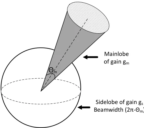
Antennaradiation patternshows the angular dependence of the gain values, and is typically depicted as a 3-D graph, or separate projections in the vertical and horizontal planes. In a radiation pattern plot, theantenna beamwidth means the angle between the half-power (-3 dB) points of the direction of peak gain. Beamwidth is usually expressed in degrees for the horizontal plane. In this dissertation, the mainlobe (ML), or main beam, is defined as the lobe within the half-power beamwidth of the peak gain, and the rest are side lobes (SLs).

3.2.2 Anisotropic Radiation Pattern of Omni-directional Antenna

For most RSSI range-based localization algorithms, an assumption is made that the antenna radiation pattern is perfectly circular in shape. It is assumed, in this case, that the formula for RSSI attenuation over distance, as described by the log shadow model, is directly applicable. However, in the real world, the pattern of radio transmitted at the antenna is not a circular shape.

(30)

Figure 3.2: Measured horizontal radiation patterns in dBs for indoor (blue solid line) and in chamber environment (red dashed line).

1 m from the receiver, in both indoor environment and the anechoic chamber. As shown in Figure 3.2, the radiation patterns are far from omni-directional and with differences in the measured RSSI of over 20 dBm.

3.2.3 Directional Antenna Models

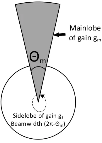
Precisely modeling real antennas with main and side lobe characterization is difficult and also not the main scope of this work, therefore we utilized a simplified antenna pattern introduced in [48]: the antenna pattern consists of one mainlobe of beamwidthθm, with gain gm, and one

sidelobe of beamwidth (2π−θm) with gaings. In a 3-D visualization as shown in Figure 3.3, the

side lobes are the solid arc with radius proportional to the power radiated by the radiator, and the cone is the mainlobe, which is circular in cross section. In this work, our target network is 2-D, therefore we are more interested in the horizontal projection of the 3-D radiation pattern, which is shown in Figure 3.4.

(31)

Θ

m

Mainlobe of gain gm

Sidelobe of gain gs

Beamwidth (2π-Θm)

Figure 3.3: 3-D radiation pattern for simplified directional antenna model.

when we change the beamwidth θm, the mainlobe gain gm and sidelobe gain gs needs to be

carefully chosen to ensure that the total radiated energy is constant. Consider the radiation pattern shown in Figure 3.3, all the power radiated from the mainlobe is constrained to flow through a circular surface section on the sphere. Letr be the radius of the sidelobe solid arc, the radius of the circular section can be obtained asr·θm/2. LetP be the total radiated power

over all directions,S be the surface area of the sphere, andM be the surface area falls within the main beamwidth. Using (3.2) and the fact that total energy has to remain equal, we have following constraints:

gm·U ·M+gs·U·(S−M) =η·P, (3.4)

S = 4πr2_, _(3.5)

M =π(r·θm/2)2, (3.6)

(32)

Mainlobe

of gain g

m

Sidelobe of gain gs Beamwidth (2π-Θm)

Θ

m

Figure 3.4: Radiation pattern projection in horizontal plane for a two dimensional directional antenna model.

For a given θm, when we assume that only a negligible amount of radiated power is diverted

into the sidelobe, the maximum mainlobe gain is:

D= 16 θm2

, (3.8)

and D is often called as thedirectivity of the antenna. Otherwise, we can choose a gm smaller

thanD, and consequently gs is:

gs=

η·D−gm

D₋1 . (3.9)

gs=

η_· 16

θm2 −gm

16

θm2 −1

(33)

Chapter 4 KickLoc: Simple, Distributed

Localization for Wireless Sensor

Networks

In this chapter, Section 4.1 introduces details of the proposed algorithms. Section 4.2 presents simulation results, showing that the proposed system performs better than existing algorithms and close to optimum (obtained from the Cram´er-Rao bound), while requiring considerably fewer resources than existing algorithms. Finally, summary of this chapter is shown in Sec-tion 4.4.

4.1 KickLoc System Design

In this chapter, a network is formed by randomly deployed nodes, which use short range RF transceivers to broadcast messages to nodes within transmission range. Nodes that are able to directly communicate with each other are called neighbors.

(34)

uncertainty. The algorithm is fully distributed: each unknown node only communicates with its one hop neighbors throughout the broadcasting process, and upon receiving an update packet, a node performs a simple computation without having to store the information from the packet.

4.1.1 Information Exchange

Assume there are m beacon nodes (with known positions) and n unknown nodes (with un-known positions) in a randomly deployed network. For simplicity, we limit the topology to two dimensions, but our approach is capable of operating in three dimensions. Figure 4.1 shows an example network with six nodes; an edge is drawn between each pair of nodes that can directly communicate with each other. Each node periodically broadcasts its own position and precision estimate; each node receiving such a message updates its estimate. An RSSI value is also obtained with the broadcast message, and therefore a distance measurement with a cer-tain precision can be obcer-tained from the extracted RSSI. We model the distance as a normal distribution with the true distance as the mean [43]. In what follows, we present two different (but closely related) algorithms for providing updated position and precision estimates upon receiving an update from a neighboring node.

y

₆

(35)

4.1.2 KickLoc Intuitive Algorithm

At each unknown nodei, the algorithm maintains the current positionXˆi(ˆxi,yˆi) and its

stan-dard deviation ˆσi. At the start of the algorithm, the standard deviation of an unknown node is

set to infinity (in practice we set it to a large number, 10000 in simulation), and the standard deviation of a beacon node is set to 0. The initial position estimation of an unknown node is set to be the center of the deployment area. When an unknown node receives a broadcast mes-sage from a neighboring nodej, containing that neighbor’s current position Xˆj(ˆxj,yˆj) and its

standard deviation ˆσj, the distance measurement ˆdji and its standard deviation ˆσji will also be

obtained from the extracted RSSI. The unknown node can then calculate the expected distance to the neighbor using their estimated positions:

h(Xˆi,Xˆj) =

ˆ Xi−Xˆj

, (4.1)

where k·k is the Euclidean distance function. If there’s any difference between the expected distance h(Xˆi,Xˆj) and the distance measurement ˆdji, the receiving node has to update its

current position estimate, which we term “kick” to a more likely position. The new estimated position is an adjustment from the current estimation. The intuition behind the adjustment is shown in Figure 4.2. The adjustmentKick is defined as:

Kick=α·∆d·lji, (4.2)

where,

• ∆dis the residual, which reflects the discrepancy between the expected distanceh(Xˆi,Xˆj)

and the actual measurement ˆdji:

(36)

ˆ

X

i

( ˆ

x

i

, ˆ

y

i

)

ˆ

X

j

( ˆ

x

j

, ˆ

y

j

)

ˆ

d

_ji

Expected distance

h

( ˆ

X

_i

, ˆ

X

_j

)

Measured distance

(a)

ˆ

Xi

( ˆ

x

_i

, ˆ

y

_i

)

ˆ

X

j

( ˆ

x

j

, ˆ

y

j

)

ˆ

d

_ji

Expected distance

h

( ˆ

_X

_i

, ˆ

_X

_j

)

Measured distance

(b)

(37)

• lji is the direction vector of length 1 from node j to node i:

lji=

ˆ Xj−Xˆi

Xˆi−Xˆj

; (4.4)

• α is a confidence value determined by the current standard deviation of i’s position es-timation and the standard deviation of the update, which provides an estimate of the accuracy of the update:

α= σˆcurrent

ˆ

σcurrent+ ˆσupdate

. (4.5)

Intuitively, the higher the confidence in the current estimate (i.e., small ˆσcurrent), the

smaller the coefficient α is and the corresponding adjustment. Similarly, the higher the confidence of the update (i.e., small ˆσupdate), the larger the adjustment will be.

• the standard deviation of the update depends both on ˆσjiand ˆσj, where ˆσjiis the standard

deviation of the range measurement betweeniand j, and ˆσj is the standard deviation of

j’s position estimation:

σupdate=

q

ˆ σ2

ji+ ˆσ2j. (4.6)

After the adjustmentKickis calculated, Nodei’sa posteriori position estimation and standard deviation are updated as follows:

ˆ

Xpost_i =Xˆpre_i +Kick, (4.7)

ˆ

σi =α·σˆupdate+ (1−α)·σˆcurrent. (4.8)

(38)

can be determined by a preset tolerance value ∆, i.e., the process stops when

r

ˆ

Xpost_i 2−Xˆpre_i 2 ≤∆. (4.9)

In our simulations, a preset tolerance value (∆ = 0.05) is used unless otherwise specified. Figure 4.3 shows the algorithm that runs on each unknown node. The beacons only broadcast their positions.

Input:

Upon receipt of a broadcast from a neighbor node j:Xˆj(ˆxj,yˆj), ˆσj, ˆdji and ˆσji.

Output:

Node imaintainsXˆi(ˆxi,yˆi) and ˆσi.

Initialization: ˆ

Xi ←center of the deployment area

ˆ

σi← a very large number

set a periodic timer for broadcast

when a broadcast packet is received: updateXˆi and ˆσi using (4.7) and (4.8)

when the periodic broadcast timer expires: broadcast the current Xˆi(ˆxi,yˆi) and ˆσi

if reached ∆ or reachedMAX ITERATION NUM

endlocalization

end if

Figure 4.3: KickLoc Intuitive algorithm that runs on unknown nodei.

4.1.3 KickLoc Kalman Algorithm

(39)

mea-surement data (i.e., distance meamea-surement ˆd), and prior knowledge about node positions (i.e., position estimates of nodes Xˆi and Xˆj). An extended Kalman filter can be used to determine

the optimal update as we assume both the measurement model and the estimation states can be described using a Gaussian noise model.

In the KickLoc Kalman version (we call it KK in following sections.), each unknown nodei maintains its current positionXî(ˆxi,yî) with its error covariancePî, and will update both once

it receives a packet from its neighbor j containing that neighbor’s current position Xˆj(ˆxj,yˆj)

with its covariance Pˆj and the range estimate ˆdji with its variance ˆσji2. The new position

estimation is the current position adding an adjustment:

ˆ

Xi =Xˆi+K·∆d, (4.10)

where,

• ∆dis the residual, which reflects the discrepancy between the expected distanceh(Xˆi,Xˆj)

and the actual measurement ˆdji,

∆d= ˆdji−h(Xˆi,Xˆj) +w. (4.11)

• the random variable w in (4.11) represents the distance measurement noise, which is assumed to be normal:

p(w)∼ N(0,σˆ_ji2); (4.12)

• the adjustment Kis the gain that minimizes the covariance after the update.

If the estimated distance h(Xˆi,Xˆj) is linear, then (4.1) becomes:

h(Xˆi,Xˆj) =Hi·Xˆi+Hj·Xˆj, (4.13)

(40)

Kand Pˆi are given by:

K= PˆiHi

|

HiPˆiHi|+HjPˆjHj|+ ˆσ2ji

, (4.14)

and

ˆ

Ppost_i = (I−KHi)Pˆprei . (4.15)

However, in our application, the estimated distanceh(Xˆi,Xˆj) is non-linear. Specifically in 2-D,

h(Xˆi,Xˆj) is:

||Xˆi(ˆxi,yˆi)−Xˆj(ˆxj,yˆj)||=

q

(ˆxi−xˆj)2+ (ˆyi−yˆj)2. (4.16)

Hence, (4.11) has to be linearized in order to apply the extended Kalman filter. The equation for the linearization of (4.11) at point p(Xˆi,Xˆj,v) is:ˆ

dij ≈dˆij +Hi·(Xi−Xˆi) +Hj·(Xj−Xˆj) +W·(w−w),ˆ (4.17)

where

• Hi is the Jacobian matrix of partial derivatives of h with respect toXi,

Hi =

∂h ∂xi(

ˆ

Xi,Xˆj,w)ˆ _∂y∂h_i(Xˆi,Xˆj,w)ˆ

; (4.18)

• Hj is the Jacobian matrix of partial derivatives ofh with respect to Xj,

Hj =

∂h ∂xj(

ˆ

Xi,Xˆj,w)ˆ _∂y∂h_j(Xˆi,Xˆj,w)ˆ

; (4.19)

• and W is the Jacobian matrix of partial derivatives of h with respect tow,

V=

∂h

∂v(Xˆi,Xˆj,w)ˆ

= 1. (4.20)

(41)

error. The resulting K, ˆXi, and Pˆi are:

K= PˆiHi

|

, (4.21)

ˆ

Xi =Xˆi+K·∆d

=Xˆi+K·

ˆ

dij −h(Xˆi,Xˆj)

,

(4.22)

ˆ

Ppost_i =Pˆpre_i ₋KHiPˆpre_i = (I−KHi)Pˆpre_i . (4.23)

In our application, for two-dimensional coordinates with the estimated distance given by (4.16), after solving the partial derivatives of h with respect to Xi and Xj, it can be shown

thatHj =−Hi,hence HjPˆjHj|=HiPˆjHi|.Therefore (4.21) can be simplified:

K= PˆiHi

|

HiPˆiHi|+HjPˆjHj|+ ˆσji2

= PˆiHi

|

Hi(Pˆi+Pˆj)Hi|+ ˆσji2

.

(4.24)

After applying the EKF to minimize the estimation error, the resultingK, ˆXi, and Pˆi are:

K= PˆiHi

|

, (4.25)

ˆ

Xi =Xˆi+K·∆d

=Xˆi+K·

ˆ

dij −h(Xˆi,Xˆj)

,

(4.26)

ˆ

Ppost_i =Pˆpre_i ₋KHiPˆpre_i = (I−KHi)Pˆpre_i , (4.27)

whereHi,Hj are the Jacobian matrices of partial derivatives ofh with respect toXi and Xj.

In a two-dimensional application, after solving the partial derivatives ofhwith respect toXi

and Xj, it can be shown thatHj =−Hi.The covariancesPˆi,Pˆj and ˆσji2 are known, the only

(42)

h with respect toXi which can be pre-calculated off-line once for all 2-D application.

Nodeiwill store its updated position ˆXiand its precisionPˆiby overwriting the previous one,

and will repeat the update process when a new broadcast packet arrives. Using covariance matrix

ˆ

Pi and a square matrix with the number of rows and columns equal toD, the dimensionality

of the system, (i.e.,D= 2 for a 2D system andD= 3 for 3D.) The node’s standard deviation is calculated as:

σi =

v u u t

D

X

m=1

D

X

n=1

ˆ

Pi[m, n]. (4.28)

At the start of the algorithm, the error covariance Pˆ of an unknown node is set to infinity (Pˆ = ∞ 0

0 ∞

in 2-D), in practice we set it to a large number (10,000). The error covariance of a beacon node is set to 0.

4.2 Simulation Results and Analysis

The performance of the proposed approach is evaluated through simulations in MATLAB. Experimental results are presented in Section 4.3. Since standard networking issues (e.g., the routing algorithm, the transport layer, MAC fairness, etc.) do not affect the performance of our algorithm, we did not model the MAC, routing and transport layers, assuming that the updates are sufficiently infrequent to not cause congestion. In Section 4.2.1, the CRLB for multihop wireless sensor network localization is derived when the measurement distance error variance is not fixed. In Section 4.2.2, KickLoc Intuitive algorithm (KI) and KickLoc Kalman algorithm (KK) are tested in both dense and sparse networks to evaluate the number of nodes that can be localized and the performance of the algorithms. In Section 4.2.3, the convergence of each algorithm is verified first, and then bothlocalization performance andresource cost performance

of KickLoc algorithms are compared with other well-known range-based localization approaches (DV-distance [11], N-hop Multilateration [14], and IWLSE [15]). The localization precision is also compared with the CRLB.

(43)

difference between the real position of the nodes and the estimations), measured using the mean of the distance errors, and theprecision(i.e., the uncertainty of the estimations), measured using the standard deviation of the distance errors.

The three resource cost performance metrics we will be comparing are: memory cost,

com-putational cost, andcommunication cost.

Due to the random deployment of nodes, and the randomly generated error values, all scenarios have been repeated 50 times.

4.2.1 CRLB for Localization

The Cram´er-Rao lower bound is a lower bound on the variance of unbiased estimator [49]. In this paper we use it as a benchmark to evaluate the performance of our localization estimator. The approach is applicable to all algorithms that use range measurements to localize the unknowns. The derivation of the CRLB of the variance in the estimated parameters is very similar to the derivation in [44]. In the derivation in[44], the authors used a fixed varianceσ2 _{to represent} the variance of each measurement distance error. In this paper, a diagonal matrixW is used to represent the variance of each measurement since we assume that the variance of a measurement depends on the distance [15]. If the total number of measurements isM,W will be anM×M matrix:

W=diag

1 σ2

i

, (4.29)

whereσ2

i is the variance of theith measurement.

The Cram´er-Rao lower bound

The lower bound is given in terms of Fisher Information Matrix (FIM) J(θ). Let ˆθ be any unbiased estimate of parameter θ based on observation vector X having a pdf of fX(x). The

error covariance matrix is defined as:

(44)

This error covariance matrix is bounded below by the CR bound, which is given by:

CRB = [J(θ)]−1, (4.31)

where the matrix J(θ) has elements given by:

[J(θ)]mn =E

∂ln(fX(X))

∂θm

∂ln(fX(X))

∂θn

. (4.32)

Obtaining the CRB for Multihop Topologies

In the multihop problem, the parameter vectorθ of interest is the 2A×1 vector:

θ= [x1, y1, x2, y2,· · ·, xA, yA]|, (4.33)

where A is the number of unknown nodes. The measurement vector X is a M ×1 vector of distance measurements ˆdij. We assume that each measurement ˆdij is white Gaussian, and the

mean is the true distance dij with standard deviation σij.

The measurement pdf is the joint conditional pdf:

fX(X;θ) = M Y k=1 1 σk √ 2πexp

−(xk−µk)

2 2σ2 k = M Y j=1 Y

i∈H(j)

i<j 1 σij √ 2πexp (

−( ˆdij −dij)

2 2σ2 ij ) , (4.34)

where i_∈H(j) means node i is within j’s transmission range, hence a distance measurement can be obtained between the two. In matrix form:

fX(X;θ) =

s

det(W) (2π)M exp

−1

2

ˆ

d₋d|_·W_·dˆ₋d

(45)

Therefore the likelihood function is:

L(θ,X) = lnfX(X;θ)

= 1 2ln

det(W) (2π)M −

1 2

n

ˆ

d₋d|_·W_·dˆ₋do.

(4.36)

The CRLB can be computed from the FIM ofθ from (4.32):

J(θ) =E{[∇θlnfX(X;θ)] [∇θlnfX(X;θ)]|}. (4.37)

From (4.1), (4.33) and (4.34):

J(θ) =

G0(θ)|

·W·

G0(θ)

, (4.38)

whereG0(θ) is theM_×2Amatrix whosemnth _{element is} ∂µm

∂θn. Ifµm corresponds todij, since

θn is eitherxi0 oryi0 for some corresponding node i0,

G0(θ)mn=

                              

0, ifi06=iand i0 6=j

xi−xj

dij , ifθn=xi

xj−xi

dij , ifθn=xj

yi−yj

dij , ifθn=yi

yj−yi

dij , ifθn=yj.

(4.39)

The CRLB is then given by the inverse of the FIM as in (4.31). The CRLB for the localization error of theith _{unknown node can be described by:}

E

( ˆxi−xi)2+ ( ˆyi−yi)2

(46)

error of the network, RM S(σ) can be obtained by:

RM S(σ) =

v u u t

1 A

A

X

i=1

J−1

2i−1,2i−1+J

−1 2i,2i

. (4.41)

The value RM S(σ) gives the average lower bound in errors of estimated locations.

4.2.2 Performance Analysis of KickLoc

For meaningful comparisons between different parameter settings, the estimation errors are normalized to the transmission range (i.e., a relative estimation error of 0.5 means half the transmission range). We define coverage as the ratio of unknown nodes that can be localized to the total number of unknown nodes. In DV-distance, N-hop Multilateration and IWLSE, a node can get a position estimation when it is connected to at least three beacons (one-hop or multi-hop). In KickLoc, unknown nodes keep updating its position estimation regardless of the number of beacons it is connected to. In this section, we define four criteria for nodes that can be localized to investigate the trade-off between coverage and localization error. The four criteria are based on the least number of beacons it requires for a node to be localized: zero

connected beacons, one connected beacon, two connected beacons and three connected beacons.

When evaluating the performance of localization under i connected beacons criterion, we only consider the performance of the unknown nodes that are connected to at leastibeacons (single or multi-hop). Thus, for three connected beacon criterion, we only measure the performance of nodes that are connected to at least three beacons, while under the zero beacon criterion, all nodes are considered, even if completely isolated.

(47)

an unknown node. In this subsection, a preset number of iterations (20 in simulation) and dif-ferent criteria of being localized are used for better observation of convergence process; in all other sections a preset tolerance value (∆ = 0.05) and three connected beacons criterion are used unless otherwise specified.

Dense network

The first environment we test is a dense network with the following parameters: • Total number of nodes (beacons and unknowns): 200

• Area: 100m×100m • Transmission range: 30m • Beacon to total nodes ratio: 0.2

• Standard deviation of the distance measurement d, σij(d): 0.2d (20% of the distance

measurement.)

(48)

0 20 40 60 80 100 0 20 40 60 80 100 1 2 3 4 5 6 7 8 9 10 11 12 13 14 15 16 17 18 19 20 21 22 23 24 25 26 27 28 29 30 31 32 33 34 35 36 37 38 39 40 41 42 43 44 45 46 47 48 49 50 51 52 53 54 55 56 57 58 59 60 61 62 63 64 65 66 67 68 69 70 71 72 73 74 75 76 77 78 79 80 81 82 83 84 85 86 87 88 89 90 91 92 93 94 95 96 97 98 99 100 101 102 103 104 105 106 107 108 109 110 111 112 113 114 115 116 117 118 119 120 121 122 123 124 125 126 127 128 129 130 131 132 133 134 135 136 137 138 139 140 141 142 143 144 145 146 147 148 149 150 151 152 153 154 155 156 157 158 159 160 161 162 163 164 165 166 167 168 169 170 171 172 173 174 175 176 177 178 179 180 181 182 183 184 185 186 187 188 189 190 191 192 193 194 195 196 197 198 199 200

Figure 4.4: An example dense network topology with 40 beacons and 160 unknown nodes.

Relative Distance Error

0 0.5 1 1.5 2

CDF 0 0.1 0.2 0.3 0.4 0.5 0.6 0.7 0.8 0.9 1 KI KK (a)

Number of iterations

0 5 10 15 20

0 0.2 0.4 0.6 0.8 1 1.2 1.4 KI KK (b)

(49)

Sparse network

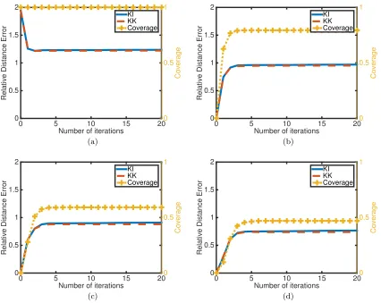
Next we evaluate the performance of the algorithms in a sparse network with a reduced number of nodes (30 instead of the 200 in the dense network) and a reduced transmission range (20m instead of 30m in the dense network).

A sample topology is shown in Figure 4.6. The simulation is repeated 100 times, and the average connectivity of the network is 3.07. Figure 4.7 illustrates the CDF of relative localization errors for the two algorithms. Underzero connected beacon criterion, KI and KK both achieve a confidence interval with confidence level 90% for the relative error of (-2.50, +2.50), and achieve the 50% accuracy of 0.75. Under one connected beacon or more criterion, KI and KK both achieve a confidence interval with confidence level 90% for the relative error of about (-1.89, +1.89), and achieve the 50% accuracy of 1.06. The coverage withone connected beacon

criterion is 79.42%, withtwo connected beacons criterion is 59.13%, andthree connected beacons

criterion is 47.00%. Figure 4.8 shows how fast the algorithms converge as the iterations go on under different beacon criteria. Both algorithms have an initial steep drop, and converge after only a few iterations.

0 20 40 60 80 100

0 20 40 60 80 100 1 2 3 4 5 6 7 8 9 10 11 12 13 14 15 16 17 18 19 20 21 22 23 24 25 26 27 28 29 30

(50)

0 0.5 1 1.5 2 2.5 3

CDF

0 0.1 0.2 0.3 0.4 0.5 0.6 0.7 0.8 0.9 1

KI (0 beacon) KK (0 beacon)

KI (1 beacon, 2 beacons, 3 beacons) KK (1 beacon, 2 beacons, 3 beacons)

Figure 4.7: CDF of relative localization error in sparse networks.

The results show that in both dense and sparse networks, both KI and KK converge after a small number of iterations. As expected, the localization errors in sparse network are much higher than in dense network, since in sparse networks with random deployment, many unknown nodes are in positions in which it is impossible to obtain an accurate location), for example if they are disconnected or far from any beacons, or in a corner. In general, KI has a similar performance to KK, though it has more relaxed assumptions (i.e., the adjustment is on the line determined by the two nodes’ position estimation). Although KK is supposed to be optimal, its performance is affected by the error introduced from the linearization process of function h(Xˆi,Xˆj): the measurement functionhis non-linear and cannot be accurately estimated by the

linearization. Furthermore, this transformation error cannot be estimated and is therefore not reflected in the estimation error covariancePˆi. Hence, a high error in one nodekwill negatively

(51)

0 5 10 15 20

0 0.5 1 1.5 2 Coverage 0 0.5 1 KI KK Coverage (a)

0 5 10 15 20

0 0.5 1 1.5 2 Coverage 0 0.5 1 KI KK Coverage (b)

0 5 10 15 20

0 0.5 1 1.5 2 Coverage 0 0.5 1 KI KK Coverage (c)

0 5 10 15 20

0 0.5 1 1.5 2 Coverage 0 0.5 1 KI KK Coverage (d)

(52)

4.2.3 Performance Comparison

With the simulator described above, a series of tests have been performed to obtain measure-ments on different performance metrics of the system. For localization performance metrics, we vary the number of nodes, area size, transmission range, beacon to total nodes ratio and dis-tance measurement error standard deviation. A set of parameter values is chosen, from which one value is changed at a time to test the systems sensitivity to that particular parameter. Table 4.1 summarizes the values chosen.

Under the standard scenario, the average connectivity of the network is 10.4224, the mean and standard deviation (µ, σ) of the relative estimation error are (0.4557, 0.4613) for KI, (0.4777, 0.4648) for KK, (0.6179, 0.3674) for DV-distance, (0.5094, 0.4053) for N-hop Multilateration, (0.5015, 0.4513) for IWLSE. The standard deviation of the relative estimation error for CRLB is 0.2337. The coverages of the 5 algorithms are 100%.

Table 4.1: Standard values and variation ranges for parameters used in the simulation.

Parameter Standard

value Range

Total number of nodes 100 20 - 200 Area size (100m)2 _(20m)2 _{- (200m)}2 Transmission range 20m 10m - 50m Beacon to nodes ratio 20% 5% - 50%

STD σij(d) 0.2d 0.05d- 0.5d

Convergence Results

(53)

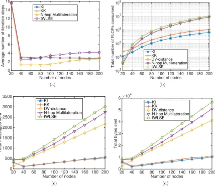
box (for N-hop Multilateration) to obtain their localization estimates. In N-hop Multilateration and IWLSE, these localization estimates serve as an initial estimate, and an iterative refinement phase follows to improve the localization performance. In KickLoc algorithms, there’s no need to establish the “DV-distance propagation” first, as the iterative refinement phase starts at the very beginning of the process. Since the localization procedure is different for each algorithm, the iteration steps cannot be directly compared for the different algorithms. To illustrate the convergence trends at different network densities, Figure 4.9(a) shows the average number of iterations for each algorithm as a function of the number of nodes in the network. All the algo-rithms converge within five iterations unless it is a very sparse network. When the network is very sparse, most of the unknown nodes cannot reach the preset tolerance value (∆ = 0.05 in simulation), hence will keep iterating until reaching the maximum preset iteration steps (20 in simulation).

Localization Accuracy and Precision

In the next series of simulations, each algorithm’s localization performance is investigated when the number of nodes, beacon to total nodes ratio and distance measurement error standard deviation are varied according to Table 4.1.

Number of nodes:Figure 4.10 shows that the relative error mean and standard deviation decrease as the number of nodes increase for all algorithms. The increasing number of nodes results in higher density network when other parameters are fixed. All algorithms work better when the network is dense because there is more available information. DV-distance and IWLSE do not perform well when the number of nodes is small, because DV-based distance correction works poorly in sparse anisotropic networks. N-hop Multilateration does not perform well at high number of nodes, because in its refinement stage, it leverages estimates from all its neigh-bors without estimation precision information. KickLoc algorithms have good performance at both low and high number of nodes.

(54)

Number of nodes

20 40 60 80 100 120 140 160 180 200

Average number of iteration steps

0 2 4 6 8 10 12 14 16 KI KK N-hop Multilateration IWLSE (a)

Number of nodes

20 40 60 80 100 120 140 160 180 200

Total number of FLOPs consumed

103 104 105 106 107 108 KI KK DV-distance N-hop Multilateration IWLSE (b)

Number of nodes

20 40 60 80 100 120 140 160 180 200

Total messages sent