Two dimensional heat transfer problem in flow boiling in a rectangular minichannel

a

Corresponding author: [email protected]

Two dimensional heat transfer problem in flow boiling in a rectangular

minichannel

Sylwia Hoejowska 1,a, Magdalena Piasecka2 and Leszek Hoejowski1

1

Kielce University of Technology, Faculty of Management and Computer Modelling, Al. 1000 – lecia P.P. 7, 25-314 Kielce Poland

2

Kielce University of Technology, Faculty of Mechatronics and Mechanical Engineering, Al. 1000 – lecia P.P. 7, 25-314 Kielce Poland

Abstract. The paper presents mathematical modelling of flow boiling heat transfer in a rectangular minichannel asymmetrically heated by a thin and one-sided enhanced foil. Both surfaces are available for observations due to the openings covered with glass sheets. Thus, changes in the colour of the plain foil surface can be registered and then processed. Plain side of the heating foil is covered with a base coat and liquid crystal paint. Observation of the opposite, enhanced surface of the minichannel allows for identification of the gas-liquid two-phase flow patterns and vapour quality. A two-dimensional mathematical model of heat transfer in three subsequent layers (sheet glass, heating foil, liquid) was proposed. Heat transfer in all these layers was described with the respective equations: Laplace equation, Poisson equation and energy equation, subject to boundary conditions corresponding to the observed physical process. The solutions (temperature distributions) in all three layers were obtained by Trefftz method. Additionally, the temperature of the boiling liquid was obtained by homotopy perturbation method (HPM) combined with Trefftz method. The heat transfer coefficient, derived from Robin boundary condition, was estimated in both approaches. In comparison, the results by both methods show very good agreement especially when restricted to the thermal sublayer.

1 Introduction

Over the recent years, the range of applications of flow boiling heat transfer through minichannels with different geometries has widened considerably and included new generations of systems. Extensive research effort to understand boiling phenomena in mini- and microchannels is reflected in numerous experimental measurements and theoretical data analyses. In addition to providing design guidance for cooling systems furnished with minichannel devices, the findings can be applied to thermostabilization and thermoregulation problems. The application of enhanced surfaces in boiling heat transfer in micro- and minichannels has not been studied sufficiently. This issue attracts attention due to theoretical enhancement potential for transferring large heat transfer fluxes.

From a great variety of computational methods applicable to the considered problem one seems to be exceptionally simple and convenient, namely Trefftz method [1] in combination with homotopy perturbation method (HPM) [2]. Both are normally used for solving problems described by partial differential equations. The idea of Trefftz method is to approximate the unknown solution of a differential equation by a linear combination

of the functions (called Trefftz functions) which satisfy the given equation identically. The coefficients of Trefftz functions should be selected to minimize the mean square error of approximation on the boundaries. In HPM the unknown solution of a differential equation is expressed as an infinite series which is supposed to be convergent to the exact solution. In practice, HPM needs only few iterations to provide accurate approximation. The combination of HPM with Trefftz method allowed to determine two-dimensional temperature distribution of the boiling liquid flowing in an asymmetrically heated horizontal minichannel.

2 Experiment

2.1 Experimental stand and measurement module

The test section with a minichannel (figure 1b, 1) 1 mm deep, 40 mm wide and 360 mm long, oriented horizontally is the most important part of the system. The heating element for FC - 72 made from alloy Haynes 230 (2) is microstructured on one side (8) and in direct contact with the fluid flowing in the channel. It is C

Owned by the authors, published by EDP Sciences, 2015

possible to observe the channel surfaces through two glass panes. One pane (4b) allows observing foil temperature changes owing to a liquid crystal layer (3) deposited on the plain side of the foil. An example of a thermographic image is shown in figure 1a. The other glass plane (figure 1b, 4a) allows conducting two-phase flow visualization on the microstructured foil side, as shown in figure 1c. K - type thermocouples are installed at the inlet and outlet of the minichannel (figure 1b, 7).

The data and image acquisition system with digital cameras, a data acquisition station, a computer with specialized software and lighting systems are the essential parts of the research equipment. The flow loop is comprised of a test section, a rotary pump, a compensating tank, a heat exchanger, a filter, rotameters and a deaerator. The schematics of the main loops and the data acquisition system of the test setup are presented in [3 - 7]

.

Figure 1. The schematic diagrams of the measurement module: 1– minichannel, 2 – heating foil, 3 – liquid crystal layer, 4a, b – glass sheet, 5– channel body, 6 –front cover, 7 – thermocouple, 8 – enhanced surface, 9 – copper element, b) thermographic images, c) two phase flow structures images; experimental parameters: mass flux 286 kg / (m2 s), inlet pressure 130 kPa, volumetric heat flux:1) 15.2⋅104 kW/ m3, 2) 19.7⋅104 kW/ m3, 3) 24.7⋅104 kW/ m3, 4) 30.5⋅104 kW/ m3, 5) 3.42⋅105 kW/ m3.

Application of the liquid crystal thermography for the detection of two-dimensional heating surface temperature distribution must be preceded using colour (hue); and temperature calibration is required. Detailed information about the accuracy of the heating foil temperature measurements with liquid crystal thermography and other experimental data errors are described in [7].

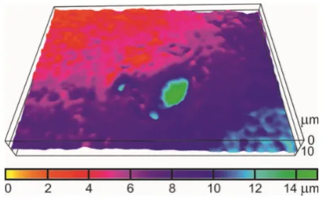
On one side of the heating foil, mini-recesses were formed and distributed uniformly on the entire foil. They are obtained by spark erosion, using electric-etcher and branding-pen (arcograph), are unevenly distributed [8]. The height and depth of the craters of these recesses depend on the parameters of branding-pen settings. The layer of melted metal of the foil and the electrode material, a few μm high, reaching locally 5 μm, accumulates around the cavities. The depth of the craters of cavities is usually below 1 μm. The exemplary 3D topography of selected sample area photo of the enhanced foil with mini-recesses is presented in figure 2.

Figure 2. 3D topography of selected enhanced sample area of the foil with mini-recesses.

2.2 Experimental methodology

FC-72 working fluid, at the temperature below its boiling point, flows laminarly into the minichannel. The gradual increase in the electric power supplied to the heating foil results in an increased heat flux transferred to the liquid in the minichannel. The current supplied via copper elements (figure 1b, 9) to the heating foil is controlled by an electrical system equipped with an inverter welder. This leads to the incipience and next to the development of nucleate boiling.

Thanks to the liquid crystal layer located on its surface contacting the glass it is possible to measure the temperature distribution of the heating wall. Flow structure observation is carried out simultaneously at the opposite side of the minichannel.

2.3 Void fraction determination

The analyses of the flow structure are based on the monochrome images of flow structures with an SLR camera of heating foil, obtained on the side contacting fluid flowing in a minichannel. They were processed using Corel graphics software.

Techsystem Globe. The software allowed the determination of the areas of the two phases and/or percentage of the defined phase. Methodology of the conversion of greyscale image into monochrome image is presented in detail in [7]. It allowed for determination of the areas of the two phases and/or the percentage of the defined phase.

In figure 3, cross-sections of binarized structure image adopted for analysis in Techsystem Globe are shown for the selected areas. Subsequent cross-sections of both images and the binarized image of two-phase flow structure image (black and white) adopted for analysis in Techsystem Globe are also shown.

The cross-sectional void fraction

ϕ

exp was

determined according to the following formula [3 - 7]:

v l

v

M v l

M v

v l

v

A A

A A

A A V V

V

+ = ⋅ +

⋅ = + =

δ δ ϕ

) (

exp

(1)

where: V – volume, A – cross section area, δ_M – channel depth; letters in subscript apply to the following phases: liquid (l in subscript) or vapour (v in subscript).

3

Mathematical model

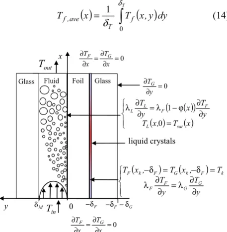
As in the approach described in [9, 10], mathematical modelling of the problem was simplified by neglecting one dimension. Only two dimensions were taken into account: x along the flow direction and y, perpendicular to the flow direction, relating to the thickness of the glass (δ_G), the foil (δ_F), and to the depth of the channel (δ_M). Additionally, we focused on the central part of the measurement module (along its length). The quantities referring to glass, foil and liquid are distinguished in notation with subscripts: G, F and f, respectively. The process of heat exchange in the glass barrier and in the heating foil is described with Laplace and Poisson equation, respectively. Thus the governing equations are

in glass: ΔTG=0 (2)

in foil:

F V F

q T

λ

− =

Δ (3)

where: qV denotes volumetric heat flux supplied to the

heating foil and λ_F – foil thermal conductivity. At the glass - foil contact we assume that both temperatures and heat fluxes must be matched, which gives

k G

F T T

T = = (4)

y T y

T _G

G F F

∂ ∂ = ∂

∂ _λ

λ (5)

k

T denotes the temperature measured at the glass - foil interface at discrete points, using liquid crystals thermography. The remaining boundaries are assumed to be isolated [11, 12], figure 4.

For the liquid we assumed that the flow was steady – state, stationary and laminar (Reynolds number Re < 2000), with a constant mass flux in the minichannel. Taking into account the effect of frictional heat, the energy equation exclusively for the liquid phase can be written as follows

f

f AT

T =

Δ (6)

where ₂

2 2 2 y x ∂ ∂ + ∂ ∂ =

Δ and a differential operator A is

given by

( )

x a y w A ∂ ∂ = (7) where: f f , p f c a ρ λ

=

.

Fluid velocity vector is parallel to

the flow direction and its y – component, w(y), has the form

( )

(

2

)

2 L y y

p y w _M f − Δ = δ

μ (8)

where L means length of the heating foil and μ_f is the dynamic viscosity of the liquid. Equation (6) is accompanied by the boundary conditions at foil-liquid contact [9,10]:

– for the liquid temperature

¯ ® ­ + ≥ + < = sup sat F sat sup sat F F f T T T , T T T T , T T if if (9)

where the saturation temperature T_sat depends on the linear pressure drop p(x) in the minichannel, and T_supis the liquid superheat that initiates boiling:

( )

(

)

f T V sup q x T λ δ ϕ −

= 1 (10)

The thickness of the thermal boundary layer δ_T is determined from the formula [13]

h

T Pr δ

δ 3 1 − = f ave f h u f ρ μ

δ = 2 ,

Re f = 64 ,

f h f ave d w Re μ ρ

= (11)

where waveis the mean velocity of the liquid.

– for bubbly and bubbly - slug flows we assumed [9, 10, 13]

( )

(

)

T_y

x y T _F F f f ∂ ∂ − = ∂ ∂ ϕ λ

λ 1 (12)

Additionally, the liquid temperatures at the minichannel inlet and outlet are known. Figure 4 depicts the

mathematical model of the problem (domain geometry and boundary conditions).

Once the heating foil and the liquid temperature distributions are known, the heat transfer coefficient

( )

x

α at the foil - liquid interface can be determined using the Robin boundary condition

( )

x

(

T T

( )

x

)

y T ave , f F F

F = −

∂ ∂

−λ α (13)

where Tf,ave is reference temperature defined as mean

temperature of the thermal layer:

( )

=

_³

( )

T dy y , x T x T _f T ave , f δ δ ₀ 1 (14) ( ) ( ) ( ) ( ) °¯ ° ® ­ = ∂ ∂ ϕ − λ = ∂ ∂ λ x T , x T y T x y T sat L F F L L 0 1 ( ) ( ) °¯ ° ® ­ ∂ ∂ λ = ∂ ∂ λ = δ − = δ − y T y T T , x T , x T G G F F k F k G F k F out T F δ

− −δF−δG

x

y δM

0 = ∂ ∂ y TG liquid crystals in T 0 Fluid Glass Glass Foil

0 = ∂ ∂ = ∂ ∂ x T x

TF G

=0 ∂ ∂ = ∂ ∂ x T x TF G

Figure 4. Scheme of the measuring module with boundary conditions (pictorial view, not to scale).

4 Solution methods

4.1 Trefftz method

Determination of two-dimensional temperature field distributions in the glass pane, in the heating foil and in the liquid was achieved with a use of Trefftz method. In the first step of a three - stage sequential procedure, the temperatures TG and TF were approximated by linear

combinations of Trefftz functions corresponding to Laplace equation, [11]:

( )

_¦

( )

= = G N i i i G x,y au x,y T 1 (15)

( ) ( )

_¦

( )

= + = F N j j j F x,y u~ x,y bu x,y T

1

(16)

( )

x,y i

θ , corresponding to energy equation written in the form

( )

x T a

y w

T_f f

∂ ∂ =

Δ (17)

with parabolic velocity profile (8), [9]. The temperature of the liquid is approximated with a sum whose first term represents a particular solution to equation (6) and the second term is a linear combination of Trefftz functions

( )

x,y i

θ

( )

_¦

( )

=

=

f N

k i i

f x,y c x,y

T

0

θ (18)

The unknown coefficients ai , bj ,ci in (15), (16) and

(17) are determined from the least squares criterion – to achieve for each of the respective functions TG, TFand Tf

the minimum of squared residuals along the domain boundaries. This procedure was thoroughly discussed in [9, 11, 12]. The Trefftz-type approximate solutions TG, TF

and Tf satisfy the respective governing equations. The

boundary conditions, however, are fulfilled in the least-squares sense.

4.2 Homotopy perturbation method (HPM)

In order to compare the results obtained by Trefftz method, the temperature of the liquid was calculated with a hybrid method combining HPM and Trefftz approach. As typical of homotopy technique, we construct a homotopy h

(

x,y,p

)

being a solution to the equation

(

1−p

) ( ) ( )

[

Δ h −Δu0

]

+p

[

Δ

( ) ( )

h −Ah

]

=0 (19)

where p is a parameter such that 0≤ p≤1 and u₀ is an initial approximation of equation (6). The development of the function h in powers of p gives

(

)

( ) ( )

( )

x,y p h

( )

x,y p ... h

p y , x h y , x h p , y , x h

+ +

+

+ +

=

3 3 2 2

1 0

(20)

By putting p = 1 in (19) we get equation (5). Hence the solution to (6) can be approximated by a truncated series

( )

_¦

( )

=

=

f N

i i f x,y h x,y T

0

(21)

The convergence HPM has been proved in [2] and the convergence rate depends on the operators Δ and A, [14]. The requirements concerning the function u₀ could be weakened. In practice, one might take an arbitrary function as u₀. The calculations by the authors of this research showed that satisfactory results can be obtained using only 3 or 4 terms in the series (21) and taking u0=0

for convenience. After substituting (20) to equation (19) we get an infinite series. We collect terms with equal

powers of p. Since the series is identically zero, all its coefficients must be equal to zero. Hence we get the successive differential equations with unknown functions

,... h , h , h0 1 2

( )

₀ =0

Δh

( ) ( )

₁ − ₀ =0

Δh Ah

( ) ( )

₂ − ₁ =0

Δh Ah (22)

...

( ) ( )

− 1 =0

ΔhN_f AhN_f−

The functions h0,h1,h2,... were found from equations (22) by Trefftz method. Each h_n

( )

x,y was represented by a linear combination of Trefftz functions u_i

( )

x,y satisfying Laplace equation, i.e.

( )

_¦

( )

=

= n

N

i i n i n x,y d u x,y h

1

(23)

From the substitution of (23) into (22) and due to linearity of differential operators Δ and A, it was possible to obtain the recurrence formula for h_n

( )

x,y . Starting with h0

( )

x,y which is derived from the first of the equations (22), we get the next functions:

( )

_¦

( )

_¦

[

(

)

]

= −

− =

Δ +

= n n _n

N

s

s N s N

i i n i

n x,y d u x,y Ah

h

1 1

(24)

where Δ−1 denotes the inverse of Δ and

( )

[

1

]

1 − − −

− _{=Δ Δ}

Δ s s

. More information on inverse differential operators can be found in [15, 16]. The boundary conditions assumed for equation (6) allow to determine the coefficients of u_i

( )

x,y in (24). The coefficients should minimize a proper error functional, specific to every h_n

( )

x,y . In the recurrence procedure for findinghn

( )

x,y , one has to modify the boundary conditions any time we pass to the next iteration. The new boundary condition depends on h_n

( )

x,y obtained in the previous step as described in [17]. Thus, from (21) we obtain the solutionTf(temperature of the liquid) which

satisfies, in an approximate manner, the governing equation (6) and the assumed boundary conditions.

5 Results

void fraction in selected cross-sections was calculated. In further calculations, the local void fraction determined at the distances of 0.09 m, 0.133 m, 0.27 m, and 0.34 m from the minichannel inlet was approximated with a quadratic function, figure 5b.

330 335 340 345 350 355

0.00 0.07 0.14 0.21 0.28 0.35

#2

#3

#4 #5 #1

a)

x / m

T

emp

er

at

u

re /

K

0% 15% 30% 45% 60%

0.07 0.14 0.21 0.28 0.35

#2 #3 #4 #5 #1

b)

x / m

v

o

id

f

ra

ct

io

n

(

)

ϕ

x

Figure 5.a) Temperature distributions at the glass - foil contact obtained with liquid crystal thermography, b) void fraction dependence along the minichannel length. Experimental parameters shown in the description of figure1; foil parameters:

δF = 1.02 ⋅ 10-4 m, L = 0.35 m, λF = 8.3 W / (m K); glass

parameters: δG = 0.006 m, λG = 0.71 W / (m K).

As follows from the developed mathematical model, two-dimensional temperature distributions in the glass pane and in the heating foil were determined first and they are presented in figure 6. The assumed conditions of a perfect thermal contact between the glass and the foil, (5) and (6), are met with very high accuracy.

d)

L b) Foil

x / m a) Glass

c) T k

a) TG b ) TF

T / K

334 337 340 343 346 349 x, m

333 336 339 342

0.06 0.09 0.12 0.15 0.18

T /

K

Figure 6. Temperature of the glass (a) and of the foil (b) obtained with the Trefftz method and temperature measurements (c); additional data as in figure 5, #4; temperature scale (d).

In the next stage, the liquid temperature distribution in the minichannel, Tf , was determined. The calculations

required the following physical quantities: local void fraction, pressure drop, liquid temperature at the inlet and outlet of the minichannel, saturation temperature and the foil temperature gradient in the foil-liquid contact area along the channel. The values of other parameters necessary for computations were the following: six Trefftz functions θ_i

( )

x,y in the expansion (18), three iterations in HPM-Trefftz iterative procedure described by (24) and five Trefftz functions u_i

( )

x,y in development (23) of every h_n

( )

x,y . As shown in figure 7 the temperatures of the liquid obtained by both methods have their distributions approximately equal to each other, especially when observed in the thermal layer.

he

at

in

g

f

o

il

he

at

ing f

o

il

fl

o

w

d

ir

ec

tio

n

a) b)

c) T / K

whole domain

330 333 336 339 342

heat

in

g f

o

il

he

at

in

g f

o

il

a)

b)

thermal layer

d) T / K

332 334 336 338 340 342

fl

o

w

d

ir

ec

tio

n

Figure 7. Temperature of the liquid obtained by: a) Trefftz method, b) HPM-Trefftz combined method; additional data: as in figure5, #4, c) and d) temperature scale.

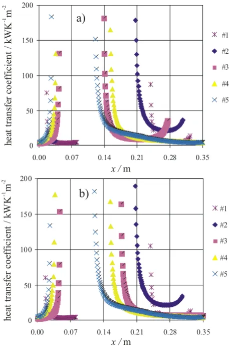
combined with Trefftz method to calculate the temperature of the liquid (figure 8b). Variation of the heat transfer coefficient along the minichannel does not exceed 200 kW K-1m-2. An increase followed by a decrease in the liquid temperature, seen in figure 5a, is caused by vapor bubbles arising in the near-wall layer and acting as internal heat outlets absorbing a considerable amount of energy transferred to the liquid. In the region of developed boiling, the heat transfer coefficient value decreases with the distance from the inlet of the channel and with the increase in the vapor fraction within the flowing mixture (figure 8).

x / m

h

ea

t t

ra

n

sf

er

co

ef

fi

ci

en

t /

k

W

K

m

-1

-2

0 50 100 150 200

0.00 0.07 0.14 0.21 0.28 0.35

#1

#2

#3

#4

#5

a)

0 50 100 150 200

0.00 0.07 0.14 0.21 0.28 0.35

#1

#2

#3

#4

#5

h

eat

t

ran

sf

er co

ef

fi

ci

en

t

/ k

W

K

m

-1

-2

b)

x / m

Figure 8. Heat transfer coefficients as a function of the minichannel length obtained by: a) Trefftz method , b) HPM - Trefftz combined method; additional data as in figure 5.

6 Conclusions

The paper presented application of two methods for solving an inverse heat conduction problem concerning forced flow boiling in a minichannel. Trefftz method was used to solve a boundary value problem in the glass pane and two inverse problems in the heating foil and in the boiling liquid. Both temperatures and heat fluxes were determined. From the known temperature distribution at the foil-liquid interface it was possible, due to Robin condition, to estimate the heat transfer coefficient.

The numerical results were compared to those obtained by hybrid HPM-Trefftz method. The resulting two two-dimensional temperature distributions in the

liquid showed good agreement, particularly when close to the thermal layer. The analogous relationship was observed in heat transfer coefficient estimated by both approaches. Some more general conclusions can be formulated from our study of the considered problem. The presented Trefftz method could be applied to solving other linear differential equations. Trefftz functions for problems described by other equations are either available or quite easy to generate. Solutions always satisfy proper differential equations and boundary conditions are satisfied in least-squares sense. The advantage of HPM-Trefftz combined method lies in its mathematical simplicity. For satisfying results only few iterations are sufficient. The method allows for treatment of problems governed by nonlinear equations. Hence, further research will be focused on estimating temperatures in more complex mathematical models of two-phase flows where gas and liquid phase and a mixture of these two phases have to be distinguished.

Acknowledgments

The research has been financially supported by the National Scientific Center granted on the basis of decision No. DEC-2013/09/B/ST8/02825.

References

1. E. Trefftz, Proc. 2nd Int. Con. App. Mech. 131-137 (1926)

2. J.-H. He, Comput. Methods App. Mech. Eng. 178 257–262 (1999)

3. M. Piasecka, Int. J. Heat and Mass Transf. 66, 72-488 (2013)

4. M. Piasecka, B. Maciejewska, Exp. Thermal Fluid Sci. 44, 23-33 (2013)

5. M. Piasecka, Heat Mass Transf. 49, 261-271 (2013) 6. M. Piasecka, Exp. Heat Transf. 27, 231-255 (2014) 7. M. Piasecka, Metrology and Meas. Sys. XX,

205-216 (2013)

8. M. Piasecka, Advanced Material Research 874, 95-100 (2014)

9. S. Hoejowska, R. Kaniowski, M.E. Poniewski, Int. J. Numer. Methods Heat Fluid Flow 24 811-824 (2014)

10. S. Hoejowska, M. Piasecka, Heat Mass Transf. 50 1053-1063 (2014)

11. S. Hozejowska, M. Piasecka, M.E. Poniewski, Int. J. Therm. Sci. 48 1049-1059 (2009)

12. M. Piasecka, S. Hoejowska, M.E. Poniewski, Int. J. Heat Fluid Flow 25 159-172 (2004)

13. T. Bohdal, Arch.Therm. 21 34-75 (2000)

14. H. Quarnia El, World J. Model. Simul. 5 225-231 (2009)

15. K. Grysa, A. Maci&g, A. Pawi'ska, Int. J. Heat Mass Transf. 55 7336–7340 (2012)

16. M. Soka*a, M.J. Cia*kowski, TRECCOP’04 251-259 (2009)