Article
Self-Tuning Method for Increasing Reliability in
Obstacle Detection based on Internet-of-Things
LiDAR Sensor Models.
Fernando Castaño 1,*, Gerardo Beruvides 1, Alberto Villalonga 1,2, and Rodolfo E. Haber 1
1 Centre for Automation and Robotics, UPM – CSIC; Arganda del Rey, 28500, Spain; [email protected]
2 Research Centre of Advanced and Sustainable Manufacturing, UM; Matanzas, 44100, Cuba; [email protected]
* Correspondence: [email protected]; Tel.: +34-918-711-900
Abstract: Nowadays, the research and development of on-chip LiDAR sensors for vehicle collision avoidance is growing very fast. Therefore, the assessment of the reliability in obstacle detection using the information provided by LiDAR sensors has become a key issue to be explored by the scientific community. This paper presents the design and implementation of a self-tuning method in order to maximize the reliability of an Internet-of-Things sensors network and to minimize the number of sensors to localize with the required accuracy obstacles by a detection threshold. In order to achieve this goal, models that predict accuracy (i.e., prediction error) for object localization using data collected by LIDAR sensors are designed and implemented in Webots Automobile 3D simulation tool. The approach is based on combining different techniques. Firstly, point-cloud clustering technique and an error prediction model library composed by a multilayer perceptron neural network with backpropagation, k-nearest neighbors and linear regression are explored. Secondly the above-mentioned techniques for modeling are also combined with a supervised and reinforcement machine learning technique, Q-learning in order to minimize the detection threshold. In addition, a IoT driving assistance simulated scenario with a LiDAR sensor network is designed in order to validate the prediction model and the optimal configuration of the sensor network to guarantee reliability in obstacle localization. The results demonstrate that the self-tuning method is appropriate to increase the reliability of the sensor network whereas minimizing the detection threshold.
Keywords: LiDAR sensors reliability; Internet of Things, self-turning parametrization; k-nearest neighbors, driven-assistance simulator.
1. Introduction
Nowadays, the Internet of Things (IoT) applications are present in many sectors from industry environments (e.g. manufacturing, energy, etc.) to our personal lives (e.g. health, society, mobility, etc.). IoT are strategic for automotive applications with fresh push and investment in recent years in order to develop and put into the market smart mobility ecosystems with an autonomous level of interaction between vehicles and infrastructures. Nevertheless, everyday car manufacturers, OEMs for automotive sector, researchers and engineers are introducing new technological contributions and new challenges should be addressed in short terms [1, 2].
One particular challenge aiming at autonomous driving is the estimation of the accuracy and reliability in vision devices such as Light Detection and Ranging (LiDAR) and stereo camera integrated into automotive driving assistance systems for pattern recognition and obstacle detection tasks [3]. In many scenarios, it is very difficult to certify with a lower uncertainty level the real topology and distance of the objects, in most cases due to phenomena as dead zones, object
transparency, light reflection, weather conditions and sensors failures [4]. Furthermore, traditional networking devices are not designed to be used in the unpredictable, varying and dynamic environments of a IoT transportation ecosystems, being necessary to develop new methodologies to characterize and estimate the sensors reliability [5]. By the other hand, sensors fusion is commonly applied to combine different sensors for road detection, mainly cameras and LiDARs. Nevertheless, current sensor fusion methods are taking advantage of both sensors (cameras or LIDARs), rather than exploiting the advantages of each sensor isolated [6]. Furthermore, the parallel processing of frames (from camera) and scans (LiDAR) imply a high computational cost, being unnecessary in many scenarios if a method of error prediction based on sensor model for assessing reliability in runtime is developed [7].
Another important issue is the increase of computing power and wireless communication capabilities to expand the role of sensors from mere data collecting to more demanding tasks as sensor fusion, classification and collaborative target tracking. Fault tolerance and reliability perform a key role for embedded systems, such as obscured wireless sensors, which are deployed in some applications where it is difficult to access them physically [8]. Reliable monitoring of a phenomenon (or event detection) depends on the set of data provided by the cluster of sensors, and not only rely on any individual node. The failure of one or more nodes may not cause the disconnection of operational data sources from the data sinks (command nodes or end user stations). However, it may increase the number of hops a data message has to go through before reaching its destination (and subsequently increase the message delay), giving an estimation of the failure probabilities of the sensors, as well as the intermediate nodes (nodes used to relay messages between data sources, and data sinks) [9].
Several reconstruction methods are reported in the literature to create specific geometry models of existing objects from scanned point clouds based on information obtained from LiDARs [10]. The progress in modelling techniques to simulate complex driving environments provides a realistic representation between multiple input/output variables in order to determinate which factors are most influential in degrading reliability, and rank ordering them, as well as, the detection of pedestrians, obstacles and vehicles in real-time driving scenarios [11]. Clustering techniques are highly used on exploratory data mining, statistical analysis, pattern recognition, image analysis, information retrieval, bioinformatics, data compression and computer graphics [12]. Among clustering algorithms one of the most used is the k-nearest neighbor’s (k-NN) algorithm because of the simplicity to get nearest neighbors of a query in training dataset, and then predicts the query with the major class of nearest neighbors [13]. Another widely applied technique in industrial applications is the reinforcement learning [14]. A good example of that are the results archived by the Q-learning algorithm in function to generate artificial intelligence and self-learning strategies on complex processes, providing self-tuning capability to obtain the optimal configuration based on the reward or penalties learned in previous states (iterative knowledge generation) [15].
From the best of authors’ knowledge, the main contributions of this work is the design and
implementation of a four-step method to maximize the reliability on IoT LiDAR sensors network and to minimize detection threshold (the number LiDAR sensors required to detect one obstacle). The method includes a point cloud grouping, modeling, learning and self-tuning (knowledge-based learning algorithm) tasks, combining supervised and reinforcement machine learning techniques and clustering. Furthermore, a IoT driving assistance scenario with a sensor network is created using Webots simulation tool to generate a LiDAR scan benchmark. Finally, the method is validated on dynamic obstacle detention scenario in order to obtain the best prediction model and optimal number of LiDAR sensors needed to guarantee reliability in the obstacles localization using these sensors.
2. Self-tuning Method for Reliability in LiDAR sensors network.
The self-tuning method for reliability in LiDAR sensors network mainly consists of a computer-aided system to enable an efficient data interchange between the data provided by IoT sensor networks managed by a control node network and external modules devoted to evaluate the behaviour of these networks. The component in charge of generating sensory data through the simulation of sensor models is called Supervisor Node Controller (SNC); while the interface with the external modules is called IoT assessment framework. Different simulation tools can be used for this purpose. On the one hand, a 3D model simulator for automotive applications and on the other hand, an external programming software with a set of toolkits to manage points cloud, clustering methods, pattern recognition algorithms and modelling strategies based on Artificial Intelligence techniques, among others.
2.1. Conceptual design
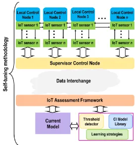
The conceptual and architectural design of the proposed method is presented in this section. Figure 2 shows the data interchange between sensory and actuation. The data interchange component operates as data sharing broker. Supervisor Node Controller (SNC) and IoT Assessment framework bring and collect information from the data interchange broker.
Figure 1. Conceptual design of Self-tuning Method. Iteration between IoT Assessment Framework and Supervisor Control Node.
The SNC is composed by different local control nodes containing Internet-of-Things (IoT) sensor network models, distributed according to their functions. The distributed IoT sensors are in charge of capturing sensory data and interchange these data with the SCN in order to share it with other external modules. It is important to highlight that to send and receive information between the different nodes of the IoT sensors network, these data must necessarily pass through the supervisor. However, this obligation is not necessary when this data transfer is between the different IoT sensors that make up the sensor network.
nodes and the IoT sensor network. The training procedure for this model is carried out using computational intelligence such as k-Nearest Neighbour, Multi-Layer Perceptron, Support Vector Machine, Self-Organizing Map, Bayesian Network, etc. For example, one model can be in charge of predicting predict the error in the localization of an object from data cloud points given by a LiDAR sensor. On the other hand, the second is group of tasks for self-tuning (knowledge-based learning algorithm). This module consists of a computational intelligence (CI) model library that contains other models with similar functions and a learning strategy (i.e., Q-Learning) that computes in runtime the actual threshold value with the aim of performing corrective actions. Both methods can also be enriched at runtime from data received by nodes of the IoT sensors network.
2.2. Implementation
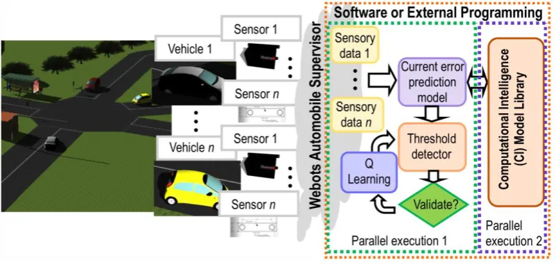
The SCN, the local control nodes and IoT sensor network are designed and implemented using a simulation tool for 3D models using Webots for automobiles R2018a [16]. In addition to its high degree of potentiality when simulating sensors for driving assistance, Webots is able to interact with other external software or programming languages, such as MatLab, Python, Java and Visual #C/C++, among others. It should be noted that for modelling and simulation of sensors, any other simulation tool for 3D sensor models can be selected.
Figure 2. Implementation of self-tuning procedure (knowledge-based learning algorithm).
Therefore, IoT assessment framework can be implemented using any of the previously mentioned software or external programming languages. However, one of these programming software with an extensive set of libraries is MaLlab 2017b, then selected for developing the self-tuning procedure. This tasks are carried out by two parallel execution threads, one of them in a local mode with directly data transfer with the IoT sensor network, and the other on a global level. The local tread (parallel execution 1) executes the current error prediction model from sensory data provided by IoT sensor network. Subsequently, depending on the value of a certain threshold that are calculated in runtime through a learning process, a set of corrective actions are performed. This procedure is described in later sections.
2.2.1. Supervisor Control Node
This controller is in charge to manage the scenario in runtime and interchange data between local control nodes or IoT sensors with other external modules. The overall operation of the 3D scenario is managed by the SCN, in this case, of Webots. Webots roots come from an extension of
robot’s simulation software adapted to automobile simulations in a virtual environment. A set of
computational procedures is in charge of adapting and transferring sensory information. The data transfer is carried out by means of different functionalities available in Webots. For example, some of available functions serves to create sensor models, such as LiDARs, stereo vison cameras, radar, Inertial, Magnetic, Gyroscope and GPS sensors that can be emulated with this software. In addition, many obstacles and objects can be added to the scenario, such as simple Vehicles, toad segments, traffic signals and lights, buildings, etc. Therefore, a 3D traffic scenario can be created in order to simulate the behaviour of IoT sensor networks that incorporates in each control local node (i.e. a fully automated vehicle) for driving-assistance scenarios.
2.2.2 Threshold detector and Q-learning procedure
Q-learning algorithm is a model-free reinforcement learning technique. Specifically, Q-learning can be used to find an optimal action-selection policy for any given (finite) Markov decision process [17]. It works by learning an action-value function that ultimately gives the expected utility of taking a given action in a given state and following the optimal policy (off-policy learner) thereafter. The algorithm is based on a simple value iteration update. It assumes the old value and makes a correction based on the new information [18].
1 1 1 1
( t , t ) ( ,t t) ( t max ( t , t) ( ,t t))
a A
Q s a Q s a gR g Q s a Q s a (1)
where, rt+1 is the reward observed after performingatin st, and is the learning rate (0 < ≤ 1).
The Q-learning algorithm is introduced in the closed-loop cycle (self-tuning) in order to minimize the numbers of LiDAR sensors needed to guarantee a good accuracy in the localization of a detected obstacle with the minimum computational illustrated in Figure 2. Table 1 shows different rewards assigned for each detection threshold ().
Table 1. Q-learning reward matrix for detection threshold.
Detection threshold () ranges
Rewards for number of LiDARs
1 3 5
0-1 1.0 0.9 0.85
1-5 0.7 0.6 0.5
5-10 0.35 0.3 0.25
+10 0.15 0.1 0
These range of values are defined in function of the obstacle prediction error calculated during the classification step (see Figure 2). During the learning process, the algorithm recommends the optimal numbers of sensors to achieve a reliable obstacle detection, based on the previous knowledge generated by the rewards obtained from similar situations learnt in the past. This self-turning threshold produces a reduction of the computational cost and an accelerates the prediction time to detect an obstacle in the driving assistance environments.
3. IoT LiDAR Sensor Models for Obstacle Detection. Case Study
same model will be used in a later section to evaluate and establish the reliability of an IoT sensor network. The way to generate a dataset for training and validate the error prediction models is described in the following sections.
3.1. Traininig dataset from 3D scenario simulation
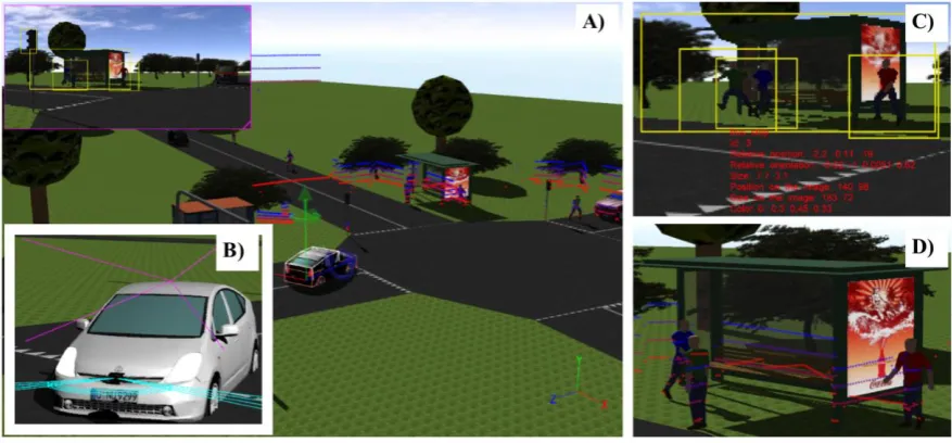
In order to generate a virtual driving traffic scenario, Webots automobile simulation tool was used, creating also a 4-layer LiDAR sensor model. The scenario emulates the real setup available in the Centre for Automation and Robotics (CAR) in Ctra. Campo Real Km. 0.2, Arganda del Rey (Madrid, Spain), composed by a test track (a roundabout, traffic lights in the central crossing and additional curves on the main straight) to simulate an urban environment with pedestrians and a fleet of six fully-automated vehicles in movement and a communications tower [19]. Figure 3 illustrates the aerial view of some of these 3D scenarios in Webots Automobile for driving assistance. A vehicle model (Toyota Prius), a camera image with objects recognized and the LiDAR point cloud are illustrated in Figure 3, implemented in this simulation tool.
Figure 3. Simulated 3D scenario in Webots for Driving Assistance. (a) Aerial view of simulation scenario, (b) vehicle model with sensors incorporated (c) camera obstacles recognition procedure
and (d) point cloud of objects into the scenario.
The fully sensorized vehicle model (Toyota Prius model) incorporates two on-board sensors, one LiDAR sensor and a 3D stereo vision camera (see Figure 3b). Both sensors are located inside the vehicle, the LiDAR on the bottom front and the camera on the upper front. Table 2 shows the specifications and localization of this sensor models into the vehicle.
Table 2. Specifications and localization into the vehicle of both sensor models.
Specifications Ibeo Lux 4 Layers Specifications Bumblebee 2 1394a
Localization Bottom frontal Localization Front top
Horizontal field 120 deg. (35 to −50 deg.) Size resolution max. 1034 x 776 pixels Horizontal step 0.125 deg. Pixel resolution 4.65 µm square pixels
Vertical field 3.2 deg. Focal lengths 3.8 mm
Vertical step 0.8 deg. Aperture Focal length / 2.0
Update frequency 12.5 Hz Frame rates 20 FPS
3.1.1. Benchmark data
During 2 minutes and 56 seconds of simulations, a data collection provided by the LiDAR sensor model and a set of captured images by 3D stereo vision camera model were obtained. In total, a benchmark of 1031 scenes is available with the same number of LiDAR scans, captured images and annotation files with the localization of each recognized obstacles.
On the one hand, the camera benchmark contains 1031 images and its corresponding annotation files obtaining from the object recognition algorithm of the camera sensor model with the following information: localization (weight x height) into the image (in pixels) of each object and the size (weight x height) of each object into the image. This model sensor is a stereo vision camera which specifications are 0.8 MP; resolution, 1032 × 776, in color and 20 FPS.
On the other hand, the LiDAR benchmark contains 1031 scans. Each scan contains 3-D point cloud/scan. This small benchmark set is useful for exploring the accuracy of an obstacle in the scene. Each scene contains in first, second and third column the X, Y, Z relative position of object regarding the localization of the LiDAR into the scene (X0 = 0, Y0 = 0 and Z0 = 0), and the fourth column are the
number of the corresponding layer.
In addition, the raw data obtained from the LiDAR need to be filtering and pre-processing in order to facilitate the determination of the error in the location of an object. Firstly, points corresponding to the ground plane that make up the road asphalts and the vegetation are eliminated. Principally, the points deleted are located 20 cm above the ground plane.
Secondly, in order to process the sensory data, fast indexing and search capabilities are required. For this, the data of the point cloud is internally organized using a k-d tree structure [20]and then, the next step of data-processing consists of extracting the points that correspond to nearby obstacles corresponding to specific point-cloud sequence. For this segmentation, a density-based spatial clustering of applications with noise (DBSCAN) was applied [21], being able to segment the point cloud for each available obstacle in the scene. Product to the algorithm returns the points clustered for each axis, the following formula is used to calculate the centroid of each point cloud segmented (X0, Y0, Z0) that corresponds to each obstacle:
0 0 0
1 1 1
( , , , ) , ,
i n i n i n
i i i
i i i
x y
X Y Z
n n n
z
(2)Finally, the last step is to compare each centroid calculated by means of the LiDAR with the actual location obtained by the object recognition algorithm of each obstacle in order to obtain the accuracy error.
Once the benchmark data set is created, the next step is to create the training data set itself for the generation of the error prediction models. Next, the spatial statistics of the point cloud used as inputs to the error prediction model are described. Subsequently, the two errors that have been taken into account as outputs of the model are also explained.
3.1.2. Model Inputs
A group of spatial statistics were implemented in order to standardize the model inputs independently of distribution of the point cloud [22]. Based on these spatial point pattern methods have been obtained the centrographic and directional distribution of the cloud of points. Common centrographic statistics for a point pattern are the mean center, median center, standard deviational circle and standard deviational ellipse [23]. The mean center MC is characterized by geographic coordinates {X, Y, Z} equal to the arithmetic means of the x-, y- and z-coordinates of all the N points in a pattern:
1 1 1
( )
;
( )
;
( )
N N N
i i i
i
x
iy
iz
MC X
MC Y
MC Z
N
N
N
An alternative unique measure of central spatial tendency of a point pattern that was used is the center of minimum distance (often referred to as the median center), which is robust in the presence of spatial outliers. Unlike the mean center, defining the median center MedC requires a much more computationally complex iterative process to find a location that minimizes the Euclidean distance d to all the points in a point pattern [24]:
,
2
2
21, 1
,
,
| min
i N t At t t t t t
i i i
i t
MedC x y z
x
x
y
y
z
z
(4)where i defines each point in a point pattern, t is an iteration number and {xt, yt, zt} is a location of an
iterative candidate median center. An important property of a point pattern is the degree of its spatial spread. It can be characterized by the standard distance SD, estimated as:
2
2
21 1 1
n n n
i i i
i i i
x
X
x
Y
x
Z
SD
N
N
N
(5)where xi, yi and zi are the coordinates of point i{xi, yi, zi}, N is the total number of points and X, Y and
Z are the coordinates of the mean center MC{X,Y,Z}.
Finally, the last spatial statistics used as input in this work is the third central moment (3thCM)
[25]. This value represents the mean value of the cubic deviation in distance of each point with respect to the mean center (MC) of each axis. The 3thCM value is calculated as follows:
2
2
21
1
3
thCM
inx
iMC X
(
)
y
iMC Y
( )
z
iMC Z
( )
n
(6)where xi, yi and zi are the coordinates of point i{xi, yi, zi}, n is the total number of points and MC is the
mean center by geographic coordinates {X, Y, Z} which were calculated in equation (3).
3.1.3. Model output
The outputs of these models are two figure of merits of the accuracy: the distance root mean squared (DRMS) and the mean radial spherical error (MRSE). The first is a measure of data tracked in the x-y plane (2D) and the second is a measure of the data tracked in x–y–z space (3D) [26]. The DRMS and MRSE values are calculated as follows:
2 2
, ,
1
1
ni Actual ti i Actual ti i
DRMS
x
x
y
y
n
(7)
2 2 2
, , ,
1
1
ni Actual ti i Actual ti i Actual ti i
MRSE
x
x
y
y
z
z
n
(8)where n is the number of readings for a dynamic tag during the time it is tracked, (xti, yti, zti) are the
coordinates of the tag at time ti, and (xActual,ti, yActual,ti, zActual,ti) are the actual coordinates of the tag at time
ti.
3.2. Model training and initial validation
composed by two hidden layer, 5 neurons for each hidden layer, sigmoid activation functions, 1∙104
epochs, training initial value of = 10–3, decrease factor of 0.1, increase factor of 10, maximum value
of was 1010 and the minimum performance gradient was 10-7. The second modeling technique is a
k-Nearest Neighbors (k-NN) with 2 neighbors. Finally, a lineal regression is also obtained by minimizing the sum of squared of the difference between the predicted and observed values.
Table 3. Model correlation coefficients based on plane & space figures of merits
Models
Correlation coefficient (R2)
DMRS MRSE
MLP 0.8668 0.8670
k-NN 0.9355 0.9355
Linear Regression 0.4841 0.4858
1031 scans were extracted from the Webots simulator to generate the training and validation datasets. Subsequently, the scans were randomly divide into two datasets: 765 samples for the training dataset (representing the 74% of the total of samples) and 255 samples to compose the validation dataset (representing the another 26% of the total of samples). The model correlation coefficients (R2) were estimated for all the models implemented in the modelling library. The Table 3
showed the values obtained for each model based on the plane (DMRS) and space (MRSE) figures of merits described before. As it can be appreciated, in both cases the k-NN algorithms represent the best fitting parameters, with a 93% of correlation between the x, y, z cloud of points coordinates in the localization of each obstacle detected.
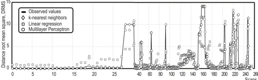
Figure 4. Prediction error behaviour of the model library in the localization of obstacles by LiDAR point clouds.
Finally, distance root mean square tendency for all the models is shown in Figure 4, validating the best fitting obtained between the observed solution and the prediction values based on the k-NN algorithm. Nevertheless, in most of cases, the MLP model present very similar behavior with the k-NN model, not so far from the linear regression model.
4. Experimental results.
Additional experimental tests, for evaluating the IoT on-chip LiDAR sensor network and the performance of self-tuning methodology on dynamic obstacle detention scenario, were also conducted in order to define the best prediction model and optimal number of LiDAR sensors required to ensure the reliability of this sensor network. Some critical conditions were taken into account in the conducted study.
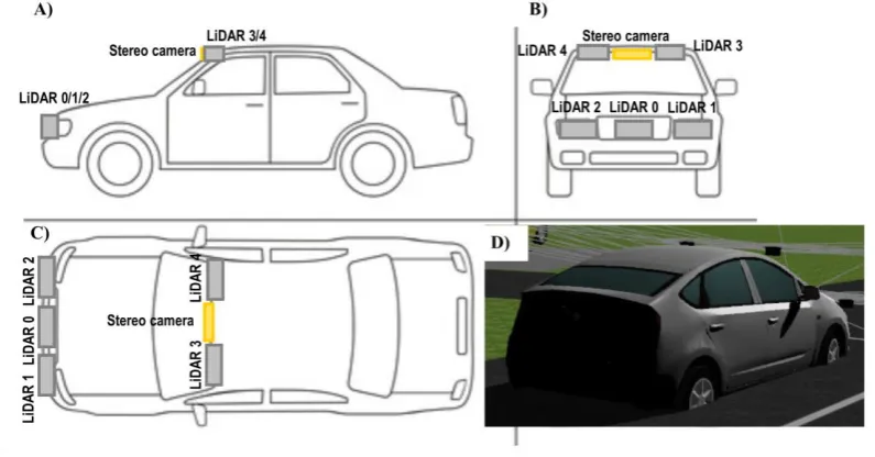
generated in section 3. However, there are more devices and objects in each scene with different distribution. Some of these dynamic objects in the scenario are 4 buildings, 50 trees, 20 pedestrians, 10 small and medium vehicles, and 1 truck. Therefore, the main difference relies on the distribution of the IoT sensory system in the fully automated vehicle (Toyota Prius) modelled in Webots (see Figure 5).
Figure 5. Side (a), front (b), plan (c) and rear view (d) of on-board IoT sensory system setup into vehicle model.
Figure 5 represents the configuration of the IoT sensory system mounted in a fully automated vehicle modelled in Webots automobile.
Table 4. Localization of each sensor which makes up the IoT sensory system.
Sensor Model Localization (m)
3D Stereo Camera Bumblebee 2 ( 0.0, 2.04, 1.2) LiDAR 0 Ibeo Lux 4 layers ( 0.0, 3.635, 0.5) LiDAR 1 Ibeo Lux 4 layers (-0.70, 3.64, 0.5) LiDAR 2 Ibeo Lux 4 layers ( 0.70, 3.64, 0.5) LiDAR 3 Ibeo Lux 4 layers (-0.55, 2.04, 1.2) LiDAR 4 Ibeo Lux 4 layers ( 0.55, 2.04, 1.2)
On the bottom front of the vehicle, three equidistant LiDAR models (LiDAR 0/1/2) are placed in order to expand the horizontal field of view. In the upper front, just on either side of the stereoscopic camera model, there are two models of LiDAR devices (LiDAR 3/4) whose purpose is to expand the field of view, in this case, vertical. The aim of this IoT evaluation is to demonstrate how IoT sensory system incorporates a series of extended capabilities in terms of precision in measurements regarding the behavior of a single sensor with better specifications than each node of the sensory network isolated. The setup of the IoT sensory system is summarized in Table 4.
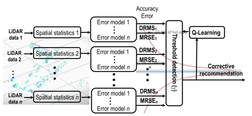
Figure 6. Flow diagram of the self-tuning method for the IoT sensors dynamic obstacle detection scenario.
During simulations of each scenario, the information provided by each sensor is collected, filtered and processed (as it was discussed in section 3.2.1), the spatial statistics are calculated (it was described in section 3.2.2) and applied as inputs to each model in the library of error prediction models. These models are able to estimate the accuracy of the localization for an object using LiDAR sensor, based on the DMRS and MRSE figures of merits. Table 5 lists the value of the correlation (R2)
of each type of model (ANN, k-NN and regression models) according to the number of LiDARs (1, 3 or 5) used at each instant with the objective of expanding the field of view, both vertical and horizontal, of the IoT LiDARs network in different critical situations.
Table 5. Behaviour of the correlation (R2) of each one of the types of models according to the number of LiDARs used at each moment.
Techniques
Model correlation (R2)
1 LiDAR 3 LiDAR 5 LiDAR
DRMS MRSE DRMS MRSE DRMS MRSE
ANN 0.8190 0.8185 0.8949 0.9167 0.8263 0.8279
k-NN 0.8184 0.8219 0.9868 0.9871 0.8893 0.8909
Regression 0.7317 0.7300 0.7572 0.7614 0.7269 0.7307
From this table, the type of model within the library with better correlation for both outputs of 2D and 3D spatial error type with respect to different IoT LiDAR system configurations can be extracted. With one LiDAR the correlation values for both outputs are similar to those obtained in section 3.2.3. On the other hand, for a configuration of 3 sensors, the value of this performance index improves notably in all models, highlighting k-NN since it is very close to 100%. Although, in theory, increasing the number of sensors the field of view is widened, it turns out that the correlation decreases with 5 sensors in all models. One of the causes of this is the duplicity of information provided by too many sensors. This problem could be solved by using an optimized distribution in mesh that avoids the duplication of space covered by each LiDAR.
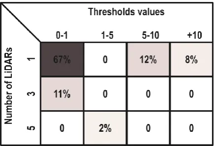
Figure 7. Q-learning classification error matrix
As it is shown, the 67% of the scenarios can be appropriately addressed with a threshold between 0-1 (in other words, with more than 99% of detection accuracy) and only one LiDAR is demanded. In total, 87% of the scenarios can be solved using only one LiDAR, but it is recommended to use 3 LiDAR if the threshold is bigger than 10 (with less than 90% of obstacle localization accuracy), increasing considerably the reliability on multi-sensor-based system. Furthermore, it is good to clarify that only in the 2% of the cases 5 LiDAR sensors are needed, which is an evidence of the suitability of the self-tuning method for minimizing the number of sensors required to achieve a higher obstacle localization reliability in the driving-assistance environments.
5. Conclusions
The design and implementation of self-tuning method based on simple soft-computing methods for automatically selecting the LiDAR sensors in a IoT multisensory driving-assistance scenarios in order to increase the obstacle localization reliability is presented in this paper. The proposed method includes four main tasks combining point cloud grouping, clustering, supervised and reinforcement learning algorithms. Three simple techniques suitable from the perspective of industrial informatics have been considered to implement the modelling library: a linear regression to corroborate the direct correlation between the extracted point clouds with obstacle localization; secondly, the well-known multi-layer perceptron once again corroborated the suitability for modelling the main process characteristics; and a k-Nearest Neighbors showing the suitability of clustering techniques to stablish correlations based on point dispersions. All the selected models have accurately reflected the behavior of the selected variables and the statistical tests have confirmed the goodness-of-fit, highlighting the more than 90% of the correlation coefficient obtained for k-NN algorithm in almost all the scenarios.
By the other hand, a Q-learning algorithm was also introduced in order to minimize the number of LiDAR sensors needed in each obstacle localization scenario to ensure sensors reliability based on global IoT sensors network information. The self-tuning procedure is based on a reinforcement learning algorithm to explore for each particular scenario how many sensors are required to detect the number of obstacles present in one scan. Based on that, the proposed method fulfils two main criteria: the best model-based fitting and self-tuning management of the computational resources (smaller number of LiDAR real required for each particular situation) necessary to improve the obstacle localization reliability on IoT LiDAR sensor networks. The accuracy and generalization of the proposed method was in a virtual driving traffic scenario developed with Webots Automobile simulation tool, solving the 67% of the scenarios taken account using one LiDAR with more than 99% of obstacle localization accuracy. Finally, the proposed self-tuning methodology will be embedded and validated in real driving environments as part of the contributions to the IoSENSE project1.
Acknowledgments: Authors wish to thank the support given by the project IoSENSE: Flexible FE/BE Sensor Pilot Line for the Internet of Everything, funded by the Electronic Component Systems for European Leadership Joint (ECSEL) Undertaking under grant agreement No 692480. http://www.iosense.eu/.
Author Contributions: Rodolfo Haber contributed with a technical and scientific review of the article whole. Alberto Villalonga was in charge of implementation of the models library and reinforcement learning algorithm. Fernando Castano and Gerardo Beruvides are designed and implemented the scenario, self-tuning methodology, and wrote the paper.
Conflicts of Interest: The authors declare no conflict of interest.
References
1. Pajares Redondo, J.; Prieto González, L.; García Guzman, J.; L Boada, B.; Díaz, V., VEHIOT: Design and Evaluation of an IoT Architecture Based on Low-Cost Devices to Be Embedded in Production Vehicles. Sensors 2018, 18, (2), 486.
2. Krasniqi, X.; Hajrizi, E., Use of IoT Technology to Drive the Automotive Industry from Connected to Full Autonomous Vehicles. IFAC-PapersOnLine 2016, 49, (29), 269-274.
3. Vivacqua, R.; Vassallo, R.; Martins, F., A Low Cost Sensors Approach for Accurate Vehicle Localization and Autonomous Driving Application. Sensors 2017, 17, (10), 2359.
4. Kempf, J.; Arkko, J.; Beheshti, N.; Yedavalli, K. In Thoughts on reliability in the internet of things, Interconnecting smart objects with the Internet workshop, 2011; 2011; pp 1-4.
5. Ahmad, M. In Reliability Models for the Internet of Things: A Paradigm Shift, 2014 IEEE International Symposium on Software Reliability Engineering Workshops, 3-6 Nov. 2014, 2014; 2014; pp 52-59.
6. Xiao, L.; Wang, R.; Dai, B.; Fang, Y.; Liu, D.; Wu, T., Hybrid conditional random field based camera-LIDAR fusion for road detection. Information Sciences 2018, 432, 543-558.
7. Zeng, Y.; Yu, H.; Dai, H.; Song, S.; Lin, M.; Sun, B.; Jiang, W.; Meng, M., An Improved Calibration Method for a Rotating 2D LIDAR System. Sensors 2018, 18, (2), 497.
8. Bein, D.; Jolly, V.; Kumar, B.; Latifi, S., Reliability modeling in wireless sensor networks. International Journal of Information Technology 2005, 11, (2), 1-8.
9. AboElFotoh, H. M. F.; Iyengar, S. S.; Chakrabarty, K., Computing reliability and message delay for Cooperative wireless distributed sensor networks subject to random failures. IEEE Transactions on Reliability 2005, 54, (1), 145-155.
10. Hu, S.; Li, Z.; Zhang, Z.; He, D.; Wimmer, M., Efficient tree modeling from airborne LiDAR point clouds. Computers & Graphics 2017, 67, 1-13.
11. Castaño, F.; Beruvides, G.; Haber, R.; Artuñedo, A., Obstacle Recognition Based on Machine Learning for On-Chip LiDAR Sensors in a Cyber-Physical System. Sensors 2017, 17, (9), 2109.
12. Shi, B.; Han, L.; Yan, H., Adaptive clustering algorithm based on kNN and density. Pattern Recognition Letters 2018, 104, 37-44.
13. Zhang, S.; Cheng, D.; Deng, Z.; Zong, M.; Deng, X., A novel kNN algorithm with data-driven k parameter computation. Pattern Recognition Letters 2017.
14. Połap, D.; Kęsik, K.; Książek, K.; Woźniak, M., Obstacle Detection as a Safety Alert in Augmented Reality Models by the Use of Deep Learning Techniques. Sensors 2017, 17, (12), 2803.
15. Haber, R. E.; Juanes, C.; del Toro, R.; Beruvides, G., Artificial cognitive control with self-x capabilities: A case study of a micro-manufacturing process. Computers in Industry 2015, 74, 135-150.
16. Michel, O., Cyberbotics Ltd. Webots™: professional mobile robot simulation. International Journal of Advanced Robotic Systems 2004, 1, (1), 5.
17. Greedy Q-Learning. In Encyclopedia of the Sciences of Learning, Seel, N. M., Ed. Springer US: Boston, MA, 2012; pp 1388-1388.
18. Chincoli, M.; Liotta, A., Self-Learning Power Control in Wireless Sensor Networks. Sensors 2018, 18, (2), 375.
19. Artuñedo, A.; del Toro, R.; Haber, R., Consensus-Based Cooperative Control Based on Pollution Sensing and Traffic Information for Urban Traffic Networks. Sensors 2017, 17, (5), 953.
21. Ester, M.; Kriegel, H.-P.; #246; Sander, r.; Xu, X., A density-based algorithm for discovering clusters a density-based algorithm for discovering clusters in large spatial databases with noise. In Proceedings of the Second International Conference on Knowledge Discovery and Data Mining, AAAI Press: Portland, Oregon, 1996; pp 226-231. 22. Lisitsin, V., Spatial data analysis of mineral deposit point patterns: Applications to exploration targeting. Ore Geology Reviews 2015, 71, 861-881.
23. De Smith, M. J.; Goodchild, M. F.; Longley, P., Geospatial analysis: a comprehensive guide to principles, techniques and software tools. Troubador Publishing Ltd: 2007.
24. Burt, J. E.; Barber, G. M.; Rigby, D. L., Elementary statistics for geographers. Guilford Press: 2009.
25. Premebida, C.; Ludwig, O.; Nunes, U. In Exploiting LIDAR-based features on pedestrian detection in urban scenarios, 2009 12th International IEEE Conference on Intelligent Transportation Systems, 4-7 Oct. 2009, 2009; 2009; pp 1-6.