Article 2
Fault Diagnosis of Induction Machines in Transient
3Regime Using Current Sensors with an Optimized
4Slepian Window
5Jordi Burriel-Valencia1,†, Ruben Puche-Panadero1,†*ID, Javier Martinez-Roman1,† ID, Angel
6
Sapena-Bañó1,† ID and Manuel Pineda-Sanchez1,† ID
7
1 Universitat Politècnica de València; [email protected];[email protected]; [email protected]; 8
[email protected]; [email protected] 9
* Correspondence: [email protected]; Tel.: +34-646-885-768 10
† Current address:Institute for Energy Engineering, Universitat Politècnica de València, Cmno. de Vera s/n, 11
46022 Valencia, Spain 12
13 14
Abstract: The aim of this paper is to introduce a new methodology for the fault diagnosis of induction 15
machines working in transient regime, when time-frequency analysis tools are used. The proposed 16
method relies on the use of the optimized Slepian window for performing the short time Fourier 17
transform (STFT) of the stator current signal. It is shown that for a given sequence length of finite 18
duration the Slepian window has the maximum concentration of energy, greater than can be reached 19
with a gated Gaussian window, which is usually used as analysis window. In this paper the use 20
and optimization of the Slepian window for fault diagnosis of induction machines is theoretically 21
introduced and experimentally validated through the test of a 3.15 MW induction motor with broken 22
bars during the start-up transient. The theoretical analysis and the experimental results show that the 23
use of the Slepian window can highlight the fault components in the current’s spectrogram with a 24
significant reduction of the required computational resources. 25
Keywords: fault diagnosis; condition monitoring; short time Fourier transform ; Slepian window; 26
prolate spheroidal wave functions; discrete prolate spheroidal sequences; time-frequency distributions 27
1. Introduction 28
Rotating electrical machines cover a broad range of applications in modern industrial installations. Particularly, cage induction machines are the most widely used due to its robustness and low maintenance requirements. Ensuring their proper functioning is essential to keep the production processes running [1]. Thus, the early detection of induction machine (IM) faults and the machine condition prognosis are crucial to reduce maintenance costs [2] and to avoid costly, unexpected shut-downs [3]. Fault diagnosis via the current analysis in the frequency domain has become a common method for machine condition evaluation because it is non-invasive, it requires a single current sensor, either a current transformer, a Hall sensor, or a magnetoelectric current sensor [4], and it can identify a wide variety of machine faults [5,6]. Traditionally, these techniques, known as motor current signature analysis (MCSA), have focused on the detection of faults during the steady state functioning of the machine through the current spectrum, which can be computed using the fast Fourier transform (FFT) [7–10]. For example, bar breakages in the rotor cage produce components of frequencies fbb[9,11–16]
fbb=|(1±2ks)|fsupply k=1, 2, 3 . . . , (1)
a mixed eccentricity fault generates components of frequencies fecc[17–19]
fecc=
1±k1−s p
fsupply k=1, 2, 3 . . . , (2)
and bearing faults generate components of frequencies fbear[20–22]
fbear=|(1±k f0)| k=1, 2, 3 . . . , (3)
wheresis the slip, fsupplyis the frequency of the power supply,pis the number of pole pairs, and fo 29
corresponds to one of the characteristic vibration frequencies generated by the bearing fault, which 30
depends on the bearing dimensions and on the mechanical rotor frequency [8,23]. However, in many 31
applications the slip, the supply frequency and the mechanical rotor frequency can be variable, which 32
render traditional MCSA techniques inadequate for fault diagnosis of electrical machines working 33
in non-stationary conditions, such as start-up transients, continuous changes in load or speed [24], 34
or variable frequency supply, especially in machines fed through variable speed drives (VSD). This 35
inadequacy resides in the FFT being unsuitable to identify fault frequencies that are no longer constant. 36
To extend MCSA to such working conditions, recently, transient MCSA (TMCSA) techniques 37
have been developed using different approaches. One approach relies on using only time-domain 38
features to isolate and to detect the fault: first the fault components of the current are extracted, using 39
a band-pass filter tailored to the frequency band spanned by the fault harmonics during the transient 40
conditions of the machine; and, second, the RMS value of these components is used to detect the fault. 41
In [25,26] the empirical mode decomposition (EMD) is used to extract the fault components. In [27] the 42
recursive undecimated wavelet packet transform (RUWPT) is used to isolate and to compute the RMS 43
value of the components produced by a broken bar fault, using an extremely low sampling frequency 44
(224 Hz) and a small number of current samples (1024 samples). Other approaches rely on tracking 45
the evolution of the fault harmonics in the time-frequency domain, looking for characteristic patterns 46
of each type of fault, as indicated by (1), (2) and (3); this technique allows the detection of different 47
types of faults, even in the case of mixed faults, with the instantaneous presence of two faults, such as 48
broken rotor bars in the presence of the intrinsic static eccentricity; as [28] states, rotor bars breakage 49
causes the static eccentricity and it is possible that two faults occur simultaneously. TMCSA techniques 50
have been developed in the technical literature using different time-frequency (TF) signal analysis 51
tools [9,29], such as the discrete wavelet transform (DWT) [15,30–36], the discrete wavelet packet 52
transform (DWPT) [37], the discrete harmonic wavelet transform (DHWT) [38], the continuous wavelet 53
transform (CWT) [39,40], the complex CWT [41,42], and the Wigner-Ville distribution (WVD) [43,44], 54
among others. Wavelet-based transforms require a proper choice of the mother wavelet and a precise 55
adjustment of the sampling frequency and the number of bands of the decomposition to perform fault 56
diagnosis. Quadratic-based transforms, such as the WVD, have, as main drawback, the appearance 57
of the cross-terms effects that can smear the spectrogram of the current signal. The minimization of 58
cross-terms effects has been widely discussed in the technical literature [43–47]. However, in the case 59
of the STFT [44,48], which can be considered the natural extension of FFT-based MCSA techniques, the 60
cross-terms effects do not appear, as the STFT is a linear transform. The STFT, as the WVD, can obtain 61
a TF distribution with enough resolution to discriminate the different harmonic components of the 62
signal, but without cross-terms effects[3]. Thus, a STFT based approach is proposed in this paper. 63
The STFT is defined as [49]
Sf(t,ω) = Z
i(τ)g(t−τ)e−jωτdτ, (4)
wherei(t)is the stator current andg(t)is the analysis window. The spectrogramPSP(t,ω)is given by
which can be re-written as [50]
PSP(t,ω) = 1
2π Z Z
Wi(τ,ν)Wg(τ−t,ν−ω)dτdν, (6)
whereWi(t,ω)andWg(t,ω)are the WVD of the stator current and the analysis window respectively.
64
Thus, the spectrogram can be considered as the 2D smoothing of the WVD of the current signal by the 65
WVD of the analysis window [51]. In other words, the window involves smoothing the oscillatory 66
interference between individual components which appear due to the quadratic nature of the WVD. 67
Hence, the window must be selected with the aim of highlighting the TF information of the analyzed 68
signal, and, at the same time with the goal of reducing to a minimum the smearing of the spectrogram 69
[52]. In fact, the optimal window is the one that -for a given total duration- maximizes the amount of 70
the total energy in a given bandwidth. But, as the uncertainty principle states, one cannot construct 71
any signal for which both the standard deviation in time,σt, and the standard deviation in frequency,
72
σω(i.e., the duration and the bandwidth) are arbitrarily small [53]. In fact, the minimum achievable
73
values ofσtandσωmust satisfy the Heisenberg’s inequality [53]:
74
σt·σω ≥0.5. (7)
The equality in (7) is only achieved by the Gaussian pulse of infinite length [54]. But real world 75
signals have a finite duration, and a gated Gaussian window is often not a good choice, as stated in 76
[55]. In fact, in fault diagnosis methods for IMs, the current is sampled during a limited time, so it is 77
a time-limited signal. But, besides, due to the limited bandwidth of the measurement channels, the 78
current signal is also a band-limited signal. Unfortunately, the uncertainty principle tells us that a 79
signal cannot be simultaneously time- and band-limited. A natural assumption is thus to consider 80
mathematically the current signal as an almost time- and almost band-limited signal, in the way 81
proposed in [56,57]. That is, using the model [58] of band-limited, or almost band-limited, functions 82
that are sufficiently concentrated in time for representing both the current signal and the window used 83
for analyzing it. 84
So, under this model,which is the optimal window? Thanks to the work presented in [59–61], 85
the optimal orthogonal system for representing almost time- and almost band-limited functions is 86
known. This system consists of the so called Slepians functions, also known as prolate spheroidal 87
wave functions (PSWFs), which have two remarkable properties that make them optimal for being 88
used as STFT windows: 89
• The Slepians are the band-limited functions that are the most concentrated to a fixed time 90
interval inL2-norm [62]. So, they can be considered as the optimal window for TF analysis of 91
non-stationary currents [63], because they can highlight the energy content of the current signal 92
in the joint time-frequency domain with the highest possible resolution among all the almost 93
time- and band-limited windows, including the truncated Gaussian window. 94
• Alternatively, the Slepians can be considered as the time-limited functions that are the most 95
concentrated to a fixed frequency interval inL2-norm. That is, for a given bandwidth they are
96
the shortest possible windows that can be used for generating the current spectrograms, which 97
allows the reduction of the time needed to build such spectrograms. 98
Both properties, the increase of the resolution of the current spectrogram and the reduction of 99
the computing time needed to obtain it, will be assessed in the experimental section of this paper. 100
The Slepian windows have been used in other fields such as medical image diagnostics [64], wireless 101
transmission [65], acoustics [66], signal processing [67], etc. But, in spite of their benefits, up to the best 102
knowledge of the authors, they have never been used before for the fault diagnosis of IMs through the 103
analysis of the stator current. 104
Therefore, the main goals of this work are, first, to introduce theoretically the Slepian window; 105
provide criteria for optimizing the parameters of the Slepian window depending on the type of the 107
diagnosed fault. The broken bar fault is used in this paper to present the application of the Slepian 108
window for the fault diagnosis of IMs, without any loss of generality, because the proposed method is 109
valid for the diagnosis of any IM fault that generates a characteristic series of harmonics in the stator 110
current, such as (1), (2) and (3). 111
This paper is structured as follows: in Section2the Slepian window is theoretically introduced 112
and compared with the Gaussian window in terms of energy concentration. Section3presents the 113
proposed procedure for using the Slepian window for fault diagnosis; for illustrating this method, it is 114
applied to a synthetic signal simulating the evolution of the left sideband harmonics (LSH) produced 115
by a broken bar during the start-up transient of an IM. In Section4the proposed approach is validated 116
using a high-power, high-voltage IM with a rotor broken bar fault. In Section5the practical advantages 117
of the proposed method are highlighted. In this section it is proposed the use of a truncated Slepian 118
window, which is able to display correctly the evolution of the fault harmonics in the TF domain with 119
a huge reduction of the computational resources needed to obtain the spectrogram. In Section6the 120
main conclusions of this work are presented. 121
2. The Slepian Functions for Fault Diagnosis of Rotating Electrical Machines in Transient Regime 122
From (6) it can be seen that the analysis window has a major effect in the spectrogram of the 123
current. It highlights the harmonic components of the current, but, at the same time, it smears the 124
spectrogram (6), so it has a major impact in the reliability of the fault diagnostic procedure. The election 125
of a window maximally confined to a region of the TF plane with a limited duration and bandwidth is 126
crucial to obtain a high resolution spectrogram, which accurately reflects the fault components of the 127
current in the TF plane, with a minimum of the smearing due to use of the window. So, the spectrogram 128
obtained with this optimal window can improve the diagnostic decision process, compared with the 129
use of non-optimal windows. The type of windows that are optimally and maximally concentrated, 130
for a finite duration and bandwidth, are the Slepians [61,68]. Accordingly, in this paper, the Slepian 131
window is proposed for the fault diagnosis of IMs. In the following subsections its characteristics and 132
the procedure to adjust its parameters are presented. 133
2.1. Theoretical introduction to the Slepian functions 134
The Slepians functions are defined [55,69,70] as the solutions of the integral equation
Z T
−Tϕ
(x)sinB(t−x)
π(t−x) dx=λϕ(t) (8)
for eigenvaluesλ=λn. There are infinite eigenvalues, all of them real numbers, positive and smaller
than 1,
1>λ0>λ1>· · ·>λn >· · ·>0. (9)
The integral equation (8) states that trimming the Slepian function of ordern, ϕn(t), with a 135
rectangular window in the[−T,T]interval will reproduceϕn(t), except for a factorλn. Besides, the 136
convolution kernel sin(Bt)/πtin (8) represents a sharp low-pass filtering process in the frequency
137
domain. Hence,ϕn(t)is a low-pass function with almost no energy at angular frequencies outside the 138
interval [−B,B]. 139
The Slepians have the remarkable property of orthogonality, both over an infinite and a finite range of the independent variable [68]. Due to the fact that the functionsϕn(t)form a complete set of orthonormal functions, band-limited functionsy(t)can be expanded in terms of the Slepians with the same bandwidth as
y(t) = ∞
∑
k=0where
ak =
Z ∞
−∞y(t)ϕk(t)dt. (11)
Other remarkable property of the Splepians is that, as the Gaussian functions, each Slepian function,ϕn(t), is proportional to its Fourier transform (FT), ˆϕn(ω), in a finite interval
ˆ
ϕn(ω)≈ϕn
t= T Bω
for |ω|<B, (12)
whereTis half of the total duration andBis the positive bandwidth (in rad/s), equal to half of the total bandwidth. Using (10) and (12), a time-limited signaly(t)can be expanded in terms of the FT of the functionsϕk(t), ˆϕk(ω), which vanish for−T<t<T
y(t) = ∞
∑
k=0bkϕˆk B
Tt
. (13)
where
bk=
Z ∞
−∞y(t)ϕk(t=
T
Bω)dt. (14)
The main application of the Slepian functions is the design of band-limited signals with a 140
maximum energy concentration in a given time and frequency interval. In the next subsections, 141
the energy concentration of a Slepian window for a given duration and bandwidth is obtained, first 142
separately in each domain, and, afterwards, in the joint TF domain. 143
2.2. Energy of the Slepian windows in a time interval 144
Given a band-limited signal,y(t), it can be expanded into the properly scaled functionsϕk(t)(10). Taking into account the orthonormality of the Slepian functions [55]
Z ∞
−∞ϕk(t)ϕj(t)dt=
(
1 if k= j
0 if k6=j (15)
the total energyEof the signal can be computed as
E= Z ∞
−∞|y(t)|
2dt=
∑
∞k=0
a2k. (16)
The energy of the signaly(t)contained in the time interval of duration(−T,T),ET, is given by
ET =
Z T
−T
|y(t)|2dt=
∑
∞k=0
λka2k. (17)
From (16) and (17), the energy fractionα=ET/Eis
α= ∑
∞
k=0λka2k ∑∞k=0a2k
. (18)
So the band-limited window which is maximally concentrated to a time interval(−T,T)is given 145
by the maximum value of the ratio (18). Sinceλ0is greater than any otherλk, this is achieved by setting 146
allakexcepta0equal to 0 [55]. Hence,αmax =λ0, whereλ0depends on the time-bandwidth product
147
(B·T). For example, ifB·T =1 thenα≈0.6. On the contrary, ifαis required to be as high as 0.95
148
thenB·T ≈3 [60,61]. So, among all the band-limited functions with the same bandwidth, the zero 149
order Slepian function,ϕ0(t), is the maximally concentrated one for a given duration.
2.3. Energy of the Slepian windows in a frequency interval 151
The energy of the signaly(t)contained in the frequency interval of bandwidth (−B,B),EB, is given by
EB=
Z B
−B
|yˆ(ω)|2dω, (19)
and, applying (13) and (14), the energy fractionβ=EB/Eis equal to
β= ∑
∞
k=0λkb2k ∑∞k=0b2k
. (20)
As done in the previous subsection, sinceλ0is greater than any otherλk, the maximum ratio (20)
152
is achieved by setting allbkexceptb0equal to 0 [55]. So, among all the time-limited functions with the
153
same duration, the zero order Slepian function,ϕ0(t), is the maximally concentrated one for a given
154
bandwidth. 155
2.4. Energy of the Slepian windows in the joint TF domain 156
As can be deduced from (18) and (20), the largest energy concentration both in the time and in the frequency domains, considered independently, is achieved by the zero order Slepian function,ϕ0(t).
Similarly, in the joint TF domain, the zero order Slepian function is also the function with the largest possible product of energy fractions,α·β, which is obtained forα=β, as in [55]
(α·β)max=
1+√
λ0
2 2
. (21)
2.5. Comparison between the Slepian window and the Gaussian window 157
The Gaussian windowg(t)is defined as [49]
g(t) =γ π
1/4 e−
γt2
2 , (22)
being
γ= 1
2σt2 . (23)
As in the case of the Slepian window, the FT of the Gaussian window, ˆg(ω), is a scaled version of
itself [49]
ˆ g(ω) =
1
γπ
1/4 e
−ω
2
2γ , (24)
where
γ=2σω2 . (25)
The Gaussian window of infinite length is optimal in terms of minimization of (7), but, for a 158
finite duration and for a given bandwidth, the zero order Slepian function achieves the maximum 159
concentration of energy in the joint TF domain. For example, forλ0=0.6, (B·T≈1), the product of
160
energy fractions (21) is(α·β)max =0.787 in the case of the Slepian window. The Gaussian window 161
has infinite length and infinite bandwidth, so for computing the energy fractionsαandβthe values of
162
half of the total durationTand half of the total bandwidthBhave been chosen as the values of the 163
respective standard deviations, as in [55]. That is,T=σtandB=σω. With these settings, the product
164
(α·β)for the Gaussian window is only about 0.466 [55].
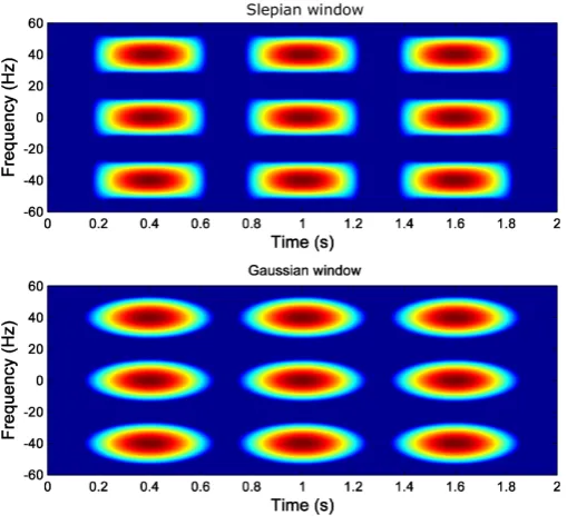
Fig.1shows the Heisenberg boxes of the Slepian and of the Gaussian atoms in the TF plane. 166
The Slepian atom has a rectangular shape, while the Gaussian atom extends radially from its center. 167
Besides, the rectangular shape of the Slepian atom allows an efficient tiling of the TF domain, and is 168
specially well suited for the proposed diagnostic approach, just by choosing the diagonal of the Slepian 169
window to be parallel to the fault component trajectory in the TF plane [54], as will be developed in 170
the next subsection. 171
Figure 1.Time-frequency atoms of a Slepian window (top) and of a Gaussian window (bottom).
2.6. Proposed method for the choice of the parameters of the Slepian window 172
In this subsection, the method for selecting the parameters that optimize the Slepian window 173
for detecting a given fault is presented. As the frequencies of the different faults in (1), (2) and (3) are 174
given in Hz, it is advisable to define this optimal window using its total bandwidth expressed in Hz, 175
that is,BW= 22Bπ =
B
π. Besides, the implementation of the STFT algorithms rely on the length of the
176
window, so it is advisable also to characterize the Slepian window using its total duration in seconds, 177
TW =2T, as depicted in Fig.2. 178
Based on the characteristics of the Slepian window in terms of energy concentration in a limited time-frequency region, the first criterion to determine the window parameters is to establish the maximum energy concentration desired for the window,(α·β)max, which imposes the time-bandwidth
product,BW·TW. In this paper an energy concentration as high as possible is proposed, i.e.(α·β)≈1,
which, from (21), givesλ0≈1. According to [60], this can be obtained with a time-bandwidth product
BW·TW =8
(α·β)max ≈1→λ0≈1→BW·TW=8 (26)
However, there are infinite combinations ofBWandTWthat meet condition (26), so an additional criterion is needed to establish bothBWandTW. These two parameters can be selected according to different criteria. In [71] the optimal bandwidth of the window for signals with time-varying frequency is found to be equal to the square root of the derivative of the instantaneous frequency (IF) of the signal. In [54,72] the optimal parameters of the Gaussian window are those that minimize the TF area occupied by a target component. To achieve this optimization, in this work the Slepian window is selected to have the maximum overlap with the trajectory of the fault harmonic signal in the TF plane, as in [54,73]. This condition is met when the magnitude of the slope of this trajectory,ρf ault, and the
aspect ratioBW/TWof the Heisenberg’s box of the Slepian window coincide (Fig.2), so that BW
TW
=ρf ault=
d(ff ault(t)) dt
. (27)
Hence, combining (26) and (27), the two conditions proposed for selecting the optimal parameters of the Slepian window are
BW·TW = 8 BW
TW
= ρf ault
(28)
From (28), the optimal length of the Slepians window is given by
TW = s
8
ρf ault
(29)
which is valid for any type of fault. For example, ρf ault can be computed from (1), (2) and (3) for the detection of rotor broken bar, mixed eccentricity and bearing faults, respectively. In the following sections the proposed approach has been applied to the diagnosis of rotor broken bars, as in [9,11,13,15,32,74], without any loss of generality. In this case,ρf aultis calculated as the derivative of (1) with respect to the time. Taking into account thats= ns−n
ns , wherenis the mechanical speed of the rotor (rpm) andns =60fsupply/pis the synchronous speed of the machine, this derivative gives, in the case of constant fsupply,
ρf ault=
d((1±2ks)fsupply) dt
=2k fsupply ds dt
= 2k fsupply ns dn dt = kp 30 dn dt
k=1, 2, 3 . . . (30)
That is, the slope of the broken bar fault harmonic at every time instant is simply the acceleration 179
of the machine at that instant, up to a constant scale factor. 180
The slope of the trajectory of the fault harmonic in the TF plane is computed at the center of the 181
Slepian window, shown in Fig.2, as in [75]. Assuming a low variation of the IF of the fault harmonic 182
during the short duration of the window, a first order, linear approximation of this trajectory can be 183
used, as in [76]. In case of long-term variations of the IF, the original current signal can be divided into 184
a number of time segments where this approximation can be applied, as suggested in [75] and [77]. 185
there is a function that returns a Slepian sequence named dpss (discrete prolate spheroidal sequences), which can be called as
dps_seq = dpss(seq_length, time_halfbandwidth, 1), (31)
where seq_length is the length of the Slepian window in samples, and time_halfbandwidth is equal to BW·TW/2. Applying (28) and (29) to (31), the optimum Slepian window for detecting a given fault is obtained easily as
dps_seq=dpss(round fsampling× s
8
ρf ault !
, 4, 1), (32)
when using a sampling frequency fsampling. 186
3. STFT of the Start-up Current of a Simulated IM using the Slepian Window 187
In this section, the use of a Slepian window for the analysis of the current through the STFT is 188
presented, and it is illustrated using the LSH generated during the start-up of a simulated machine 189
with a rotor broken bar, whose main characteristics are given in AppendixA. The simulation has been 190
performed during 2 seconds using a sampling frequency of 5 kHz, giving a total of 10000 samples. 191
3.1. Evolution of the LSH during the start-up transient of an IM 192
The evolution of the LSH of a IM with a broken bar during the start-up transient has been analyzed 193
in [9,15,79,80]. In this work, the LSH evolution is extracted from the current signal of a simulated 194
machine. Basically, the LSH fault component is a sinusoidal signal whose amplitude and frequency 195
vary continuously depending on the slips. 196
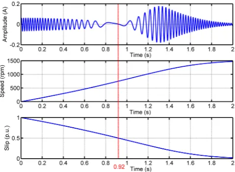
The LSH amplitude (Fig.3) follows a characteristic evolution. First the amplitude decreases until 197
it disappears (slips=0.5, timet=0.92 s). During the second half of the start-up transient (t>0.92 s) 198
the amplitude increases up to a maximum value, and, after, decreases towards its steady-state value. 199
Figure 3.Time evolution of the amplitude of the LSH (top), of the motor speed (middle), and of the motor slip (bottom) during the start-up transient of the simulated IM given in AppendixA. The vertical line corresponds to the time when the slips=0.5 is reached.
The frequency of the LSH varies as shown in Fig.4. The initial frequency of the LSH, ats=1, is 200
the same as the supply frequency (fsupply=50 Hz), and, after, it decreases, becoming null when the 201
rotor slip is equal to 0.5. From this point, the frequency of the LSH increases again, keeping a constant 202
Figure 4.Evolution of the frequency of the LSH as a function of the rotor slip.
Traditional MCSA methods cannot be used for the diagnosis of this fault in transient regime. In 204
the spectrum of the LSH shown in Fig.5, there is no peak signaling the presence of LSH, because 205
its frequency is not constant. Hence, the FFT cannot properly highlight the TF evolution of the fault 206
harmonic component generated in the stator current by the fault. 207
Figure 5.Spectrum of the LSH.
3.2. Choice of the Parameters of the Slepian Window 208
The aim of this section is to build a Slepian window suitable for identifying the LSH during the start-up transient of the IM. As deduced in Section2.6, this implies to calculate the parametersBW,TW from (28), and consequently, a value ofρf aulthas to be adopted. In this work, the value ofρf aultin (28) will be taken as its average value during the start-up transient. This is a reasonable assumption whenever the acceleration of the machine during the start-up is quite regular, as happens if the inertia factor is not very low (see Fig.3). An approximated value of the averaged value ofρf aultfor the LSH is
obtained from (30), takingk=1,
ρf ault≈2fsupply
∆s ∆t
s=0.5
s=1
=2fsupply
0.5−1 ts=0.5−0
= fsupply
ts=0.5 , (33)
or, also,
ρf ault≈2fsupply
ns
∆n ∆t
n=ns
n=0
≈ fsupply
wherets=0.5is the time which takes the rotor to reach half of the synchronous speed, andtstartupis the start-up time. Therefore, the maximum overlapping conditions (28) and (33) are combined with the level of maximum energy concentration (26), giving
BW·TW = 8 BW
TW
= ρf ault= fsupply
ts=0.5
(35)
In this case, for the simulated machine, from Fig.3,ts=0.5=0.92 s, and thusBW/TW=50/0.92= 209
54.35 Hz/s. Therefore, the parameters of the optimal Slepian window are BW = 20.85 Hz and 210
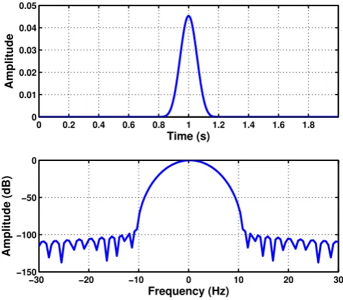
TW =383.7 ms. This window is represented in separated time and frequency planes in Fig.6, located 211
at the center of the respective domains. Almost all the energy of the window is concentrated under the 212
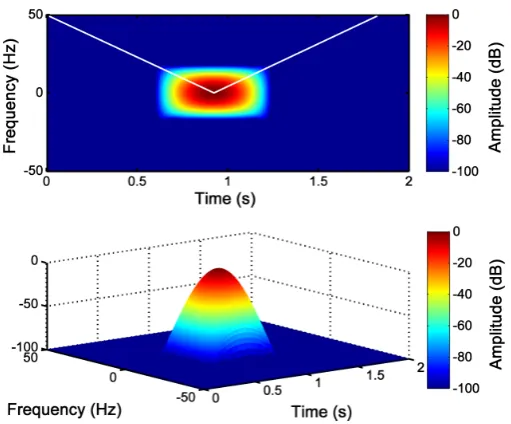
main lobe of the window in the frequency domain. On the other hand, in Fig.7, the designed Slepian 213
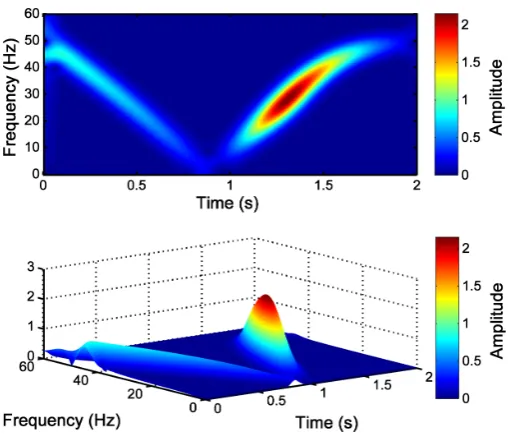
window has been represented in the TF plane, in 2 and 3 dimensions. Moreover, the slope of the LSH 214
has been superimposed (white line) in Fig.7, showing that the designed window is optimal for this 215
signal, because it achieves the maximum overlapping with the fault component trajectory in the TF 216
plane. 217
0 0.2 0.4 0.6 0.8 1 1.2 1.4 1.6 1.8 0
0.01 0.02 0.03 0.04 0.05
Time (s)
Amplitude
−30 −20 −10 0 10 20 30
−150 −100 −50 0
Frequency (Hz)
Amplitude (dB)
Figure 7.Slepian window (BW=20.85 Hz,TW=383.7 ms) optimized for representing the LSH, as a 2-D view (top) and as a 3-D view (bottom) in the time-frequency plane. The white line marks the trajectory of the LSH in this plane.
The assumption of linear instantaneous frequency during the start-up transient is quite accurate 218
in the case of large IMs (for which the condition monitoring is especially interesting), or IMs driving 219
constant loads. In case of non-linear instantaneous frequency (IF) during the start-up, the total starting 220
time can be sliced in time intervals with nearly constant IF slope (a first order approximation), as 221
done in [81]. During each one of these time intervals, the procedure for selecting the parameters of 222
the Slepian windows presented in this section can be applied, taking the value ofρf aultin (28) as its 223
average value in the interval. 224
3.3. Detection of the LSH Fault Component with the Slepian Window 225
Once the window parameters have been selected using (35), the Slepian window has been applied 226
to obtain the STFT of the LSH fault component shown in Fig.3. As it is shown in Fig.8, a high 227
resolution image of the TF pattern of the LSH (Fig.4) has been obtained with this window. Besides, 228
a linear scale has been used to represent the LSH spectrogram, so that the amplitude evolution of 229
the LSH is visible. Initially, its amplitude decreases until it becomes null (s= 0.5,ts=0.5 = 0.92 s).
230
During the second half of the start-up the amplitude increases reaching a maximum, an finally it 231
decreases again towards the steady-state value. So, the generated pattern can identify not only the 232
instantaneous frequency of the LSH, but also its instantaneous amplitude, improving the reliability of 233
Figure 8.Time-frequency-amplitude pattern generated by the LSH obtained with the optimized Slepian window (BW=20.85 Hz,TW=383.7 ms), as a 2-D view (top) and as a 3-D view (bottom).
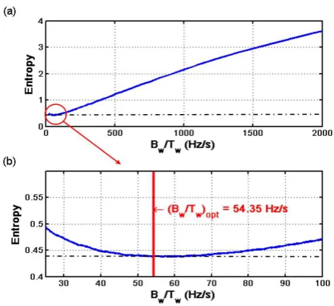
In this particular case,the optimal Slepian window has been achieved forBW/TW =54.35 Hz/s. 235
The validity of this particular choice and the sensitivity of the method to variations of this parameter 236
can be assessed measuring the entropy of the current spectrogram obtained with different Slepian 237
windows, because small entropy values correspond to good energy concentrations [82,83]. The 238
entropy of the current spectrogram has been computed with the method presented in [54,84]. Fig.9
239
shows the entropy of the LSH analyzed with the Slepian window forBW·TW = 8 (level of energy 240
concentration) and for different values ofBW/TW, from 0 to 2000 Hz/s. As can be seen in Fig.9, the 241
criterion used to select the optimal value ofBW/TWof the Slepian window,(BW/TW)opt=54.35 Hz/s, 242
corresponds indeed to the choice of the minimum entropy (maximum energy concentration) of the 243
LSH representation in the TF plane. Besides, the entropy around the optimal value is a smooth curve, 244
as can be seen in Fig.9. This indicates that the computation process ofBW/TWin (28) can tolerate 245
small errors in determining the value ofρf ault, which depends on thets=0.5value in (35). In this way,
246
in the case of motors whose speed cannot be measured, it is still possible to use an estimated value of 247
the time corresponding to a slip of 0.5 p.u. (ts=0.5), equal to half of the total duration of the start-up
248
Figure 9.a) Entropy of the time-frequency analysis of the LSH using the Slepian window, as a function of the parameterBW/TW. b) Zoomed area of the entropy in the interval close to the optimum value ofBW/TW. The vertical line corresponds to the minimum entropy value, which coincides with the criteria of maximum overlapping between the Slepian window and the LSH, as proposed in this paper.
4. Experimental Validation on a High-Power, High-Voltage IM 250
The proposed method has been applied to the analysis of a high power (3.15 MW), high voltage 251
(6 kV) IM working in an actual power plant, whose data are given in AppendixB. This IM has no 252
sensor for speed measurement. The IM had a rotor broken bar, confirmed by visual inspection of the 253
rotor (Fig.10). On the other hand, in the same factory, another IM of same characteristics was installed. 254
This second IM has not been reported for any anomaly and, thus, is meant to be in healthy condition. 255
Nevertheless, it has never been subjected to a visual inspection of the rotor. The tests have been carried 256
out during the start-up of the faulty and also of the healthy machine, powered directly from the mains 257
(fsupply = 50 Hz). The sampled current during the start-up of the faulty machine is shown in Fig.11. 258
Both tests have been performed during 8.2 seconds using a sampling frequency of 6.4 kHz, with a total 259
amount of 52480 samples. 260
Broken bar
Healthy bar
Figure 11. Stator current during the start-up transient of the high-power, high-voltage IM given in AppendixBwith a broken bar fault.
4.1. Choice of the Parameters of the Slepian Window for the Tested IM 261
The parameters of the Slepian window have been selected as proposed in Section3. First, the 262
value of the productBW·TWis selected to obtain a high energy concentration, soBW·TW =8. Second, 263
the ratioBW/TWis set to be equal to the slopeρf aultof the LSH in the TF plane. For applying (35) it is 264
necessary to know the time when the slip reaches the value 0.5,ts=0.5. In this case, as the speed is not
265
measured,ts=0.5must be estimated. Nevertheless, as it is shown in Fig.9, the entropy curve around
266
the optimal value is smooth, sots=0.5can be estimated as half of the total start-up transient duration
267
(34), without penalizing the proposed diagnostic procedure. Applying this criterion to Fig.11gives 268
ts=0.5 '3s. Hence
269
BW·TW = 8 BW TW
= fsupply ts=0.5
= 50
3
→ BW = 11.55 Hz
TW = 692.8 ms (36)
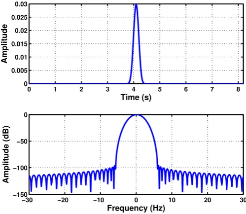
Fig.12shows the Slepian window designed in separated time and frequency domains. In Fig.13
270
an atom of the Slepian window and the trajectory of the LSH are drawn in the TF plane. As can be 271
seen, this window shape achieves the maximum overlap with the LSH trajectory, which coincides with 272
0 1 2 3 4 5 6 7 8 0
0.005 0.01 0.015 0.02 0.025 0.03
Time (s)
Amplitude
−30 −20 −10 0 10 20 30
−150 −100 −50 0
Frequency (Hz)
Amplitude (dB)
Figure 12.Slepian window (BW=11.55 Hz,TW=692.8 ms), optimized for detecting the LSH during the start-up of the high-power, high-voltage IM given in AppendixB, represented in the time (top) and in the frequency (bottom) domains.
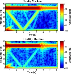
Figure 14.Spectrogram of the stator current computed with the proposed Slepian window, optimized for detecting the LSH during the start-up of the high-power, high-voltage IM given in AppendixB, with a broken bar (top) and in healthy conditions (bottom).
4.2. Application of the Slepian Window to the Fault Diagnosis of the Tested IM 274
After the selection of the parameters of the Slepian window, it has been applied to the STFT 275
of the motor stator current, to obtain the spectrograms shown in Fig.14for both the faulty and the 276
healthy IMs. In these cases, as the mains component has a much higher value than the amplitude of 277
the LSH, a logarithmic scale (dB) has been applied to the spectrogram. In Fig.14the characteristic 278
V-shaped signature of the LSH in the TF plane appears clearly for both IMs. Nevertheless, as expected, 279
the amplitude of the harmonic component corresponding to a rotor broken bar fault is much greater 280
in the case of the faulty IM (Fig.14, top) than in the case of the healthy IM (Fig.14, bottom), whose 281
V-shape corresponds to its inherent asymmetry. Fig.14gives a visual representation, which enables a 282
qualitative diagnosis. To add a quantitative criterion and to improve the reliability of the diagnosis, 283
the amplitude of the ridges of the LSH during the start-up of both machines has been represented in 284
Fig.15. In this figure, it can be seen that the LSH of the faulty machine has greater amplitude (more 285
than 10 dB) than the LSH of the healthy machine. 286
Additionally, the average values of the LSH have been computed in healthy and faulty conditions. 287
In the case of the healthy machine, the average amplitude of the LSH is−56.36 dB, whereas in the case 288
of the faulty machine it is−41.67 dB, which corresponds to a higher level of energy that confirms the 289
Figure 15.Amplitude of the LSH due to rotor broken bar during the start-up of a healthy and faulty machine extracted from Fig.14. The average value of the LSH of the healthy machine (blue line) is
−56.36 dB, and of the faulty machine (red line) is−41.67dB.
5. Cost Effective IM Fault Diagnosis Using the Truncated Slepian Window 291
In fault diagnostic systems the spectrogram of the current is not computed on the continuous TF domain, as indicated in (5), but on a discrete grid of points of the TF plane, as
PSP(m·∆T,n·∆F) =|Sf(m·∆T,n·∆F)|2, n,m=0, 1, 2, 3, . . . . (37) In fact, the current signal is a discrete sequence which is acquired sampling the stator current at 292
a frequency Fsampling during an acquisition time Ts. So, the most dense grid where the current 293
spectrogram can be calculated using (37) corresponds to a value of∆T=1/Fsampling, that is, computing 294
the FFT for every sample of the current, and to a value of∆F =1/Ts, that is, using a window with 295
the length of the current signal. This gives a total number of successive FFTs to be computed equal to 296
Ts×Fsampling, each one of lengthTs×Fsamplingsamples. All the examples presented in the previous 297
sections have been computed using this dense grid. 298
From a practical point of view, this election of∆T = 1/Fsamplingand∆F = 1/Ts in (37) is not 299
the most adequate, because with these values the computing time and memory resources needed to 300
obtain the current spectrogram are very high. For example, it takes 154 seconds and 186 Mb to obtain 301
each of the current spectrograms shown in Fig.14on a personal computer (see AppendixC), which 302
makes it difficult to implement this diagnostic technique in low power or embedded devices such 303
as FPGAs or DSPs. To alleviate this problem, the spectrogram of the current signal can be obtained 304
with a window shorter than the current signal, which reduces the length of the FFTs that must be 305
performed at each time instant. Besides, since the local Fourier spectrum averages frequency variations 306
taking place in the analysis window, it is not necessary to compute the successive FFTs for every 307
sample of the discrete-time current signal, but they can be computed with some displacement [73]. 308
Therefore, decimation in time and in frequency is almost always performed [73] when computing the 309
current spectrogram. So, a practical question is to find the minimum acceptable window length and 310
the maximum acceptable shifting time that provide a high resolution diagnostic spectrogram of the 311
stator current, keeping at a minimum the effort needed to obtain it. 312
This question has not a simple answer in the case of a Gaussian window. The use of a window 313
shorter than the current signal in the TF analysis has been seldom applied, due to the increase in 314
bandwidth of the truncated window, which blurs the current spectrogram, rendering it useless. Some 315
authors have proposed to truncate the Gaussian window when its value falls below a given threshold, 316
such as 0.01% of its maximum value, or using a truncated window with a length equal to six times 317
the standard deviation of the full-length window, 6×σt. Instead of truncating the Gaussian window,
318
window, based on a factorization algorithm [85–87], but this approach has a low penetration in the 320
fault diagnosis field. 321
In this work, and thanks to the particular properties of the Slepian window (almost compact 322
support both in time and frequency of the discrete window), this problem is solved easily using an 323
innovative and very cost-effective approach: 324
• Reducing the length of the FFT to the time durationTWof the Slepian window in (35), much 325
smaller than the length of the current signalTs. That is, using a truncated Slepian window with 326
a length equal toTW, instead of the length of the current signal. This is equivalent to setting 327
∆F=1/TWin (37). 328
• Increasing the time shift of the window in successive FFTs to a value of 1/BW, whereBWis the 329
frequency bandwidth of the Slepian window in (35), much longer than the time step between 330
consecutive samples of the current, 1/Fsampling. That is, setting∆T=1/BWin (37). 331
The results obtained with the proposed approach are summarized in Table1, and particularized 332
in Table2for the example presented in Section4. It can be observed in this table a huge reduction in 333
the computational resources needed to obtain a diagnostic spectrogram when the proposed approach 334
is used. The time needed for computing the spectrogram has been reduced from 154.65 seconds to just 335
0.59 seconds (a 0.38% of the original time), and the amount of memory from 186608 kB to just 59 kB (a 336
0.03% of the original memory usage). 337
Table 1. Comparison of the parameters of the STFT of the current signal using the traditional full length analysis and the proposed reduced length TF analysis, whereTsis the length of the current signal,Fsamplingis the sampling frequency, andTWandBWare the parameters of the Slepian window obtained from (27).
Full length TF analysis Reduced length TF analysis
Window duration (s) Ts TW=8/BW
Shift step (s) 1/Fsampling 1/BW
FFT length (samples) Ts·Fsampling TW·Fsampling
Number of FFTs Ts·Fsampling Ts·BW
Table 2.Comparison of the parameters of the STFT of the current signal using the full length and the proposed reduced length TF analysis, applied to the example presented in Section4, whereTsis the length of the current signal,Fsamplingis the sampling frequency, andTWandBWare the parameters of the Slepian window obtained from (27).
Ts=8.2 s ,Fsampling=6.4 kHz,T=0.6928 s andB=11.55 Hz
Full length TF analysis Reduced length TF analysis
Window’s length (seconds) 8.2 0.6928
Shift step (s) 1.56·10−4 0.087
FFT length (samples) 52480 4434
Number of FFTs 52480 95
Time needed for computing the spectrogram (seconds) 154.65 0.59
Fig.16shows the spectrogram of the current of the faulty machine presented in Section4, obtained 338
using the traditional spectrogram (Fig.16, top), with a length of the Slepian window equal to the 339
length of the current signal, and using the proposed decimated spectrogram (Fig.16, bottom), with a 340
truncated Slepian window. Although the computing time has been greatly reduced to a 0.4% of the 341
original time, the resultant spectrogram still shows clearly the LSH component generated by the fault. 342
Time (s)
Frequency (Hz)
Full−length STFT with the Slepian window
0 1 2 3 4 5 6 7
0 10 20 30 40 50 60
Amplitude
−100 −90 −80 −70 −60 −50 −40 −30 −20 −10 0
Time (s)
Frequency (Hz)
Reduced STFT with the Slepian window
0 1 2 3 4 5 6 7
0 10 20 30 40 50 60
Amplitude
−100 −90 −80 −70 −60 −50 −40 −30 −20 −10 0
Figure 16. TF distribution of the stator current of the faulty machine presented in Section4, using the full length TF analysis with a Slepian window (154.65 seconds, 186608 kB) (top), and using the proposed reduced length TF analysis with the truncated Slepian window (0.59 seconds, 59 kB) (bottom).
5.1. Comparison between the Spectrograms Generated with the Truncated Gaussian Window and with the 343
Truncated Slepian Window 344
For comparison purposes, the spectrogram of the current of the faulty machine has been computed 345
also with a truncated Gaussian window, using the values of window’s length and time shift obtained 346
in the design of the truncated Slepian window presented in Table2. Fig.17shows that, for the same 347
length, the truncated Slepian window (Fig.17, top) generates a current spectrogram much less blurred 348
than the spectrogram generated with the truncated Gaussian window (Fig.17, bottom), thanks to its 349
greater energy concentration. In fact, in the spectrogram generated with the truncated Slepian window 350
it is even possible to observe the signature of higher order fault harmonics (the V-shape with vertex at 351
t=4 s), which are nearly indistinguishable in the spectrogram generated with the truncated Gaussian 352
Time (s)
Frequency (Hz)
Slepian window
0 1 2 3 4 5 6 7
0 10 20 30 40 50 60 Amplitude −100 −90 −80 −70 −60 −50 −40 −30 −20 −10 0 Time (s) Frequency (Hz) Gaussian window
0 1 2 3 4 5 6 7
0 10 20 30 40 50 60 Amplitude −100 −90 −80 −70 −60 −50 −40 −30 −20 −10 0
Figure 17.Reduced spectrogram of the high-power, high-voltage faulty machine given in AppendixB
with a broken bar during the start-up transient using the truncated Slepian window (top) and using the truncated Gaussian window (bottom).
6. Conclusions 354
TMCSA methods can extend the field of application of traditional MCSA methods to the fault 355
diagnosis of electrical machines working in transient conditions, such as the start-up transient of an 356
IM, by replacing the FFT with the STFT, which is able to display the signature of the fault components 357
in the TF domain. 358
Traditionally, a gated Gaussian window has been used to perform the STFT, because an infinitely 359
long Gaussian pulse achieves the minimum value of the Heisenberg’s uncertainty principle. But, in this 360
paper, it has been highlighted that there is a special function type, the Slepian function, which achieves 361
the highest energy concentration for a finite duration and a finite bandwidth. Moreover, its atoms have 362
a rectangular shape in the TF plane. Both features improve the resolution of the current spectrograms, 363
highlighting the fault components and enabling for more reliable diagnostic results. Besides, from a 364
practical point of view, an important reduction in terms of computing time and memory resources can 365
be achieved limiting the Fourier analysis to the length of the Slepian window, and shifting the window 366
in time steps equal to the inverse of the bandwidth of the Slepian window. 367
In this paper, the use of the Slepian window for performing the TMCSA of electrical machines in 368
transient regime has been proposed, for the first time up to the best of the authors’ knowledge. The 369
procedure for selecting the parameters of the Slepian window, depending on the type of the fault, has 370
been also established, and validated both with a synthetic fault component and with the tested current 371
of a high-power, high-voltage IM with a broken bar. In future works the proposed approach will be 372
applied to the detection of other types of faults such as eccentricity or bearing faults. 373
Acknowledgments: This work was supported by the Spanish "Ministerio de Economía y Competitividad" in 374
the framework of the "Programa Estatal de Investigación, Desarrollo e Innovación Orientada a los Retos de la 375
Sociedad" (project reference DPI2014-60881-R). 376
Author Contributions:This work was performed in collaboration among the authors. R.P. directed the research; 377
J.M. contributed to the theory. J.B. and A.S. designed and validated the main methods and experiments; M.P. 378
analyzed the data. 379
Appendix A Simulated IM 381
Three-phase induction machine. Rated characteristics: P = 1.1 kW, f = 50 Hz, 382
U = 230/400 V,I = 2.7/4.6 A,n = 1410 rpm, cos ϕ = 0.8.
383
Appendix B Industrial IM 384
Three-phase induction machine, star connection. Rated characteristics: P = 3.15 MW, 385
f = 50 Hz,U = 6 kV,I = 373 A,n = 2982 rpm, cos ϕ = 0.92.
386
Appendix C Computer features 387
CPU: Intel Core i7-2600K CPU @ 3.40 GHZ RAM memory: 16 GB, Matlab Version: 9.0.0.341360 388
(R2016a) 389
References 390
1. Merizalde, Y.; Hernández-Callejo, L.; Duque-Perez, O. State of the Art and Trends in the Monitoring, 391
Detection and Diagnosis of Failures in Electric Induction Motors. Energies2017,10. 392
2. Doolan Fernandes, J.; Carvalho Souza, F.E.; Cipriano Maniçoba, G.G.; Salazar, A.O.; de Paiva, J.A. Wireless 393
Monitoring of Induction Machine Rotor Physical Variables.Sensors2017,17. 394
3. Kande, M.; Isaksson, A.J.; Thottappillil, R.; Taylor, N. Rotating Electrical Machine Condition Monitoring 395
Automatio - A Review.Machines2017,5. 396
4. Bichurin, M.; Petrov, R.; Leontiev, V.; Semenov, G.; Sokolov, O. Magnetoelectric Current Sensors. Sensors 397
2017,17. 398
5. Huang, G.; Luo, Y.P.; Zhang, C.F.; He, J.; Huang, Y.S. Current Sensor Fault Reconstruction for PMSM 399
Drives.Sensors2016,16. 400
6. Medina-García, J.; Sánchez-Rodríguez, T.; Galán, J.A.G.; Delgado, A.; Gómez-Bravo, F.; Jiménez, R. A 401
Wireless Sensor System for Real-Time Monitoring and Fault Detection of Motor Arrays. Sensors2017,17. 402
7. Cablea, G.; Granjon, P.; Bérenguer, C. Three-phase electrical signals analysis for mechanical faults 403
monitoring in rotating machine systems.Mech. Syst. Signal Process.2017,92, 278–292. 404
8. El Bouchikhi, E.H.; Choqueuse, V.; Benbouzid, M. Induction machine faults detection using stator current 405
parametric spectral estimation.Mech. Syst. Signal Process.2015,52, 447–464. 406
9. Ghorbanian, V.; Faiz, J. A survey on time and frequency characteristics of induction motors with broken 407
rotor bars in line-start and inverter-fed modes. Mech. Syst. Signal Process.2015,54, 427–456. 408
10. Liu, Y.; Guo, L.; Wang, Q.; An, G.; Guo, M.; Lian, H. Application to induction motor faults diagnosis of the 409
amplitude recovery method combined with FFT.Mech. Syst. Signal Process.2010,24, 2961–2971. 410
11. Khater, F.M.; Abu El-Sebah, M.I.; Osama, M.; Sakkoury, K.S. Proposed fault diagnostics of a broken rotor 411
bar induction motor fed from PWM inverter. J. Electr. Syst. Inf. Technol.2016,3, 387–397. 412
12. Shi, P.; Chen, Z.; Vagapov, Y.; Zouaoui, Z. A new diagnosis of broken rotor bar fault extent in three phase 413
squirrel cage induction motor. Mechanical Systems and Signal Processing2014,42, 388 – 403. 414
13. Mustafa, M.O.; Varagnolo, D.; Nikolakopoulos, G.; Gustafsson, T. Detecting broken rotor bars in induction 415
motors with model-based support vector classifiers. Control Eng. Pract.2016,52, 15–23. 416
14. Li, D.Z.; Wang, W.; Ismail, F. A Spectrum Synch Technique for Induction Motor Health Condition 417
Monitoring. IEEE Trans. Energy Convers.2015,30, 1348–1355. 418
15. Ebrahimi, B.M.; Faiz, J.; Lotfi-fard, S.; Pillay, P. Novel indices for broken rotor bars fault diagnosis in 419
induction motors using wavelet transform. Mech. Syst. Signal Process.2012,30, 131–145. 420
16. Filippetti, F.; Franceschini, G.; Tassoni, C.; Vas, P. AI techniques in induction machines diagnosis including 421
the speed ripple effect.IEEE Transactions on Industry Applications1998,34, 98–108. 422
17. Verucchi, C.; Bossio, J.; Bossio, G.; Acosta, G. Misalignment detection in induction motors with flexible 423
coupling by means of estimated torque analysis and MCSA.Mech. Syst. Signal Process.2016,80, 570–581. 424
18. Pons-Llinares, J.; Antonino-Daviu, J.; Roger-Folch, J.; Moríñigo-Sotelo, D.; Duque-Pérez, O. Mixed 425
eccentricity diagnosis in Inverter-Fed Induction Motors via the Adaptive Slope Transform of transient 426
19. Yahia, K.; Cardoso, A.; Ghoggal, A.; Zouzou, S. Induction motors airgap-eccentricity detection through the 428
discrete wavelet transform of the apparent power signal under non-stationary operating conditions. ISA 429
Transactions2014,53, 603 – 611. 430
20. Prudhom, A.; Antonino-Daviu, J.; Razik, H.; Climente-Alarcon, V. Time-frequency vibration analysis for 431
the detection of motor damages caused by bearing currents. Mech. Syst. Signal Process.2017,84, 747–762. 432
21. Elbouchikhi, E.; Choqueuse, V.; Benbouzid, M. Induction machine bearing faults detection based on a 433
multi-dimensional MUSIC algorithm and maximum likelihood estimation. ISA Transactions2016,63, 413 – 434
424. 435
22. Lee, D.H.; Ahn, J.H.; Koh, B.H. Fault Detection of Bearing Systems through EEMD and Optimization 436
Algorithm.Sensors2017,17. 437
23. Bouchikhi, E.H.E.; Choqueuse, V.; Benbouzid, M. Induction machine faults detection using stator current 438
parametric spectral estimation.Mechanical Systems and Signal Processing2015,52-53, 447 – 464. 439
24. Guo, Y.; Chen, X.; Wang, S.; Sun, R.; Zhao, Z. Wind Turbine Diagnosis under Variable Speed Conditions 440
Using a Single Sensor Based on the Synchrosqueezing Transform Method. Sensors2017,17. 441
25. Delgado-Arredondo, P.A.; Morinigo-Sotelo, D.; Osornio-Rios, R.A.; Avina-Cervantes, J.G.; Rostro-Gonzalez, 442
H.; Romero-Troncoso, R.d.J. Methodology for fault detection in induction motors via sound and vibration 443
signals.Mech. Syst. Signal Process.2017,83, 568–589. 444
26. Saidi, L.; Ali, J.B.; Fnaiech, F. Bi-spectrum based-EMD applied to the non-stationary vibration signals for 445
bearing faults diagnosis. ISA Transactions2014,53, 1650 – 1660. 446
27. Keskes, H.; Braham, A. Recursive Undecimated Wavelet Packet Transform and DAG SVM for Induction 447
Motor Diagnosis. IEEE Trans. Ind. Inform.2015,11, 1059–1066. 448
28. Faiz, J.; Ebrahimi, B.M. Mixed fault diagnosis in three-phase squirrel-cage induction motor using analysis 449
of air-gap magnetic field. Progress In Electromagnetics Research2006,64, 239–255. 450
29. Boashash, B.; Khan, N.A.; Ben-Jabeur, T. Time-frequency features for pattern recognition using 451
high-resolution TFDs: A tutorial review. Digit. Signal Process.2015,40, 1–30. 452
30. da Costa, C.; Kashiwagi, M.; Mathias, M.H. Rotor failure detection of induction motors by wavelet 453
transform and Fourier transform in non-stationary condition. Case Studies in Mechanical Systems and Signal 454
Processing2015,1, 15 – 26. 455
31. Liu, Z.; He, Z.; Guo, W.; Tang, Z. A hybrid fault diagnosis method based on second generation wavelet 456
de-noising and local mean decomposition for rotating machinery. ISA Transactions2016,61, 211 – 220. 457
32. Shi, P.; Chen, Z.; Vagapov, Y.; Zouaoui, Z. A new diagnosis of broken rotor bar fault extent in three phase 458
squirrel cage induction motor. Mech. Syst. Signal Process.2014,42, 388–403. 459
33. Yang, Y.; Nagarajaiah, S. Blind identification of damage in time-varying systems using independent 460
component analysis with wavelet transform. Mech. Syst. Signal Process.2014,47, 3–20. 461
34. Yahia, K.; Cardoso, A.; Ghoggal, A.; Zouzou, S. Induction motors airgap-eccentricity detection through the 462
discrete wavelet transform of the apparent power signal under non-stationary operating conditions. ISA 463
Transactions2014,53, 603–611. 464
35. Gritli, Y.; Lee, S.B.; Filippetti, F.; Zarri, L. Advanced Diagnosis of Outer Cage Damage in 465
Double-Squirrel-Cage Induction Motors Under Time-Varying Conditions Based on Wavelet Analysis. 466
IEEE Trans. Ind. Appl.2014,50, 1791–1800. 467
36. He, W.; Zi, Y.; Chen, B.; Wu, F.; He, Z. Automatic fault feature extraction of mechanical anomaly on 468
induction motor bearing using ensemble super-wavelet transform. Mech. Syst. Signal Process. 2015, 469
54, 457–480. 470
37. Zhang, Z.; Wang, Y.; Wang, K. Fault diagnosis and prognosis using wavelet packet decomposition, Fourier 471
transform and artificial neural network. Journal of Intelligent Manufacturing2013,24, 1213–1227. 472
38. Sapena-Bano, A.; Pineda-Sanchez, M.; Puche-Panadero, R.; Martinez-Roman, J.; Matic, D. Fault Diagnosis 473
of Rotating Electrical Machines in Transient Regime Using a Single Stator Current’s FFT. IEEE Trans. 474
Instrum. Meas.2015,64, 3137–3146. 475
39. Chandra, N.H.; Sekhar, A. Fault detection in rotor bearing systems using time frequency techniques. Mech. 476
Syst. Signal Process.2016,72, 105–133. 477
40. Sugumaran, V.; Rao, A.V.; Ramachandran, K. A Comprehensive Study of Fault Diagnostics of Roller 478
Bearings Using Continuous Wavelet Transform. International Journal of Manufacturing Systems and Design 479
41. Pineda-Sanchez, M.; Riera-Guasp, M.; Perez-Cruz, J.; Puche-Panadero, R. Transient motor current signature 481
analysis via modulus of the continuous complex wavelet: A pattern approach. Energy Conversion and 482
Management2013,73, 26–36. 483
42. Xiao, Y.; Hong, Y.; Chen, X.; Chen, W. The Application of Dual-Tree Complex Wavelet Transform (DTCWT) 484
Energy Entropy in Misalignment Fault Diagnosis of Doubly-Fed Wind Turbine (DFWT).Entropy2017,19. 485
43. Wang, S.; Cai, G.; Zhu, Z.; Huang, W.; Zhang, X. Transient signal analysis based on Levenberg-Marquardt 486
method for fault feature extraction of rotating machines. Mech. Syst. Signal Process.2015,54, 16–40. 487
44. Lee, J.H.; Kim, J.; Kim, H.J. Development of enhanced Wigner-Ville distribution function. Mech. Syst. 488
Signal Process.2001,15, 367–398. 489
45. Pachori, R.B.; Nishad, A. Cross-terms reduction in the Wigner-Ville distribution using tunable-Q wavelet 490
transform. Signal Processing2016,120, 288 – 304. 491
46. Ren, H.; Ren, A.; Li, Z. A new strategy for the suppression of cross-terms in pseudo Wigner-Ville 492
distribution. Signal, Image and Video Processing2016,10, 139–144. 493
47. Damir, M.; Victor, S.; Zlatan, C. Optimizing the Reference Signal in the Cross Wigner-ville Distribution 494
Based Instantaneous Frequency Estimation Method. Procedia Engineering2015,100, 1657 – 1664. 495
48. Liu, T.; Yan, S.; Zhang, W. Time-frequency analysis of nonstationary vibration signals for deployable 496
structures by using the constant-Q nonstationary gabor transform. Mech. Syst. Signal Process. 2016, 497
75, 228–244. 498
49. Cohen, L.Time-frequency Analysis: Theory and Applications; Prentice-Hall, Inc.: Upper Saddle River, NJ, USA, 499
1995. 500
50. Hlawatsch, F.; Boudreaux-Bartels, G.F. Linear and Quadratic Time-Frequency Signal Representations. IEEE 501
Signal Processing Magazine1992,9, 21–67. 502
51. Auger, F.; Flandrin, P.; Lin, Y.T.; McLaughlin, S.; Meignen, S.; Oberlin, T.; Wu, H.T. Time-Frequency 503
Reassignment and Synchrosqueezing: An Overview. IEEE Signal Processing Magazine2013,30, 32–41. 504
52. Ma, J.; Jiang, J. Analysis and design of modified window shapes for S-transform to improve time-frequency 505
localization. Mech. Syst. Signal Process.2015,58, 271–284. 506
53. Loughlin, P.; Cohen, L. The uncertainty principle: global, local, or both?IEEE Trans. Signal Process.2004, 507
52, 1218–1227. 508
54. Riera-Guasp, M.; Pineda-Sanchez, M.; Perez-Cruz, J.; Puche-Panadero, R.; Roger-Folch, J.; Antonino-Daviu, 509
J.A. Diagnosis of Induction Motor Faults via Gabor Analysis of the Current in Transient Regime. IEEE 510
Trans. Instrum. Meas.2012,61, 1583–1596. 511
55. Schroeder, M.R.Computer speech: recognition, compression, synthesis; Vol. 35, Springer Science & Business 512
Media, 2013. 513
56. Jaming, P.; Karoui, A.; Spektor, S. The approximation of almost time- and band-limited functions by their 514
expansion in some orthogonal polynomials bases.Journal of Approximation Theory2016,212, 41 – 65. 515
57. Karoui, A. Unidimensional and bidimensional prolate spheroidal wave functions and applications. Journal 516
of the Franklin Institute2011,348, 1668 – 1694. 517
58. Landa, B.; Shkolnisky, Y. Approximation scheme for essentially bandlimited and space-concentrated 518
functions on a disk. Applied and Computational Harmonic Analysis2016. 519
59. Slepian, D.; Pollak, H.O. Prolate spheroidal wave functions, Fourier analysis and uncertainty – I. Bell 520
System Technical Journal1961,40, 43–63. 521
60. Landau, H.J.; Pollak, H.O. Prolate spheroidal wave functions, Fourier analysis and uncertainty – II.Bell 522
System Technical Journal1961,40, 65–84. 523
61. Landau, H.J.; Pollak, H.O. Prolate Spheroidal Wave Functions, Fourier Analysis and Uncertainty–III: The 524
Dimension of the Space of Essentially Time-and Band-Limited Signals. Bell System Technical Journal1962, 525
41, 1295–1336. 526
62. Hogan, J.A.; Lakey, J.D. Frame properties of shifts of prolate spheroidal wave functions. Applied and 527
Computational Harmonic Analysis2015,39, 21 – 32. 528
63. Harris, F. On the use of windows for harmonic analysis with the discrete Fourier transform. Proceedings of 529
the IEEE1978,66, 51–83. 530
64. Lindquist, M.A.; Wager, T.D. Spatial smoothing in fMRI using prolate spheroidal wave functions. Human 531
65. Zemen, T.; Mecklenbrauker, C. Time-Variant Channel Estimation Using Discrete Prolate Spheroidal 533
Sequences. IEEE Trans. Signal Process.2005,53, 3597–3607. 534
66. Bronez, T. Spectral estimation of irregularly sampled multidimensional processes by generalized prolate 535
spheroidal sequences. IEEE Trans. Acoust., Speech, Signal Process.1988,36, 1862–1873. 536
67. Du, W.; Liao, G.; Yang, Z. Robust space time processing based on bi-iterative scheme of secondary data 537
selection and PSWF method. Digital Signal Processing2016,52, 64 – 71. 538
68. Moore, I.C.; Cada, M. Prolate spheroidal wave functions, an introduction to the Slepian series and its 539
properties.Applied and Computational Harmonic Analysis2004,16, 208 – 230. 540
69. Huibin, L.; Kang, D. Energy based signal parameter estimation method and a comparative study of 541
different frequency estimators. Mech. Syst. Signal Process.2011,25, 452–464. 542
70. Slepian, D. Prolate spheroidal wave functions, Fourier analysis, and uncertainty – V: The discrete case. Bell 543
System Technical Journal1978,57, 1371–1430. 544
71. Barber, N.; Ursell, F. The response of a resonant system to a gliding tone.The London, Edinburgh, and Dublin 545
Philosophical Magazine and Journal of Science1948,39, 345–361. 546
72. Li, M.; Staunton, R. Optimum Gabor filter design and local binary patterns for texture segmentation . 547
Pattern Recognition Letters2008,29, 664 – 672. 548
73. Zielinski, T.P. Joint time-frequency resolution of signal analysis using Gabor transform. IEEE Transactions 549
on Instrumentation and Measurement2001,50, 1436–1444. 550
74. Bessam, B.; Menacer, A.; Boumehraz, M.; Cherif, H. Detection of broken rotor bar faults in induction motor 551
at low load using neural network. ISA Transactions2016,64, 241 – 246. 552
75. Yang, W.; Tavner, P.J.; Tian, W. Wind Turbine Condition Monitoring Based on an Improved Spline-Kernelled 553
Chirplet Transform.IEEE Trans. Ind. Electron.2015,62, 6565–6574. 554
76. Yang, Y.; Peng, Z.K.; Meng, G.; Zhang, W.M. Spline-Kernelled Chirplet Transform for the Analysis of 555
Signals With Time-Varying Frequency and Its Application.IEEE Trans. Ind. Electron.2012,59, 1612–1621. 556
77. Chen, S.; Dong, X.; Yang, Y.; Zhang, W.; Peng, Z.; Meng, G. Chirplet Path Fusion for the Analysis of 557
Time-Varying Frequency-Modulated Signals.IEEE Trans. Ind. Electron.2017,64, 1370–1380. 558
78. Karoui, A.; Moumni, T. New efficient methods of computing the prolate spheroidal wave functions and 559
their corresponding eigenvalues. Applied and Computational Harmonic Analysis2008,24, 269 – 289. 560
79. Rezazadeh Mehrjou, M.; Mariun, N.; Misron, N.; Radzi, M.A.M.; Musa, S. Broken Rotor Bar Detection in 561
LS-PMSM Based on Startup Current Analysis Using Wavelet Entropy Features. Applied Sciences2017,7. 562
80. Riera-Guasp, M.; Antonino-Daviu, J.; Roger-Folch, J.; Molina Palomares, M. The Use of the Wavelet 563
Approximation Signal as a Tool for the Diagnosis of Rotor Bar Failures. IEEE Trans. Ind. Appl. 2008, 564
44, 716–726. 565
81. Pons-Llinares, J.; Riera-Guasp, M.; Antonino-Daviu, J.A.; Habetler, T.G. Pursuing optimal electric machines 566
transient diagnosis: The adaptive slope transform. Mechanical Systems and Signal Processing2016,80, 553 – 567
569. 568
82. Fischer, S.; Cristobal, G. Minimum entropy transform using Gabor wavelets for image compression. Image 569
Analysis and Processing, 2001. Proceedings. 11th International Conference on, 2001, pp. 428–433. 570
83. Romero-Troncoso, R.; Saucedo-Gallaga, R.; Cabal-Yepez, E.; Garcia-Perez, A.; Osornio-Rios, R.; 571
Alvarez-Salas, R.; Miranda-Vidales, H.; Huber, N. FPGA-Based Online Detection of Multiple Combined 572
Faults in Induction Motors Through Information Entropy and Fuzzy Inference.IEEE Trans. Ind. Electron. 573
2011,58, 5263–5270. 574
84. Sejdi´c, E.; Djurovi´c, I.; Jiang, J. Time–frequency feature representation using energy concentration: An 575
overview of recent advances. Digital Signal Processing2009,19, 153–183. 576
85. Wiesmeyr, C.; Holighaus, N.; Søndergaard, P.L. Efficient Algorithms for Discrete Gabor Transforms on a 577
Nonseparable Lattice. IEEE Trans. Signal Process.2013,61, 5131–5142. 578
86. Søndergaard, P.L. Efficient Algorithms for the Discrete Gabor Transform with a Long FIR Window. Journal 579
of Fourier Analysis and Applications2012,18, 456–470. 580
87. Moreno-Picot, S.; Arevalillo-Herraez, M.; Diaz-Villanueva, W. A Linear Cost Algorithm to Compute the 581
Discrete Gabor Transform. IEEE Trans. Signal Process.2010,58, 2667–2674. 582