Structure of the Subduction System in Southern Peru from Seismic Array Data
Thesis by Kristin Phillips-Alonge
In Partial Fulfillment of the Requirements for the Degree of
Doctor of Philosophy
CALIFORNIA INSTITUTE OF TECHNOLOGY Pasadena, California
2013
2013
ACKNOWLEDGEMENTS Robert Clayton
Younghee Kim Richard Guy Paul Davis Igor Stubailo Steve Skinner Hernando Tavera Victor Aguilar Laurence Audin
ABSTRACT
Southern Peru represents a subduction transition region from normal subduction in the
Table of Contents
Table of Figures and Illustrations ...vii
Nomenclature ... vii
Chapter 1: Introduction and Summary ... 1
Chapter 1 References ... 7
Chapter 2: Normal Subduction Region ... 10
Structure of the Subduction System in Southern Peru ... 10
From Seismic Array Data... 10
Abstract ... 10
2.1. Introduction ... 11
2.2 Data, Methods, and Results ... 15
2.2.1 Receiver Functions ... 15
2.2.1.1 Receiver Function Results ... 20
2.2.1.2 Receiver Function Waveform Modeling ... 24
2.2.2 P-Wave Tomography ... 30
2.3 Discussion ... 33
2.3.1 Crustal Thickness ... 33
2.3.2 Midcrustal Structure ... 35
Conclusions ... 38
Acknowledgements: ... 39
Chapter 2 References ... 39
Chapter 3: Subduction Transition and Flat Slab ... 45
Structure of the Subduction Transition Region from Seismic ... 45
Array Data in Southern Peru ... 45
3.1. Introduction ... 46
3.2. Methods ... 50
3.2.1 Stations and Data ... 50
3.2.2 Receiver Functions ... 52
3.2.3 Finite Difference Modeling ... 54
3.3. Results ... 56
3.3.1 Line 2 Results: Transition From Normal to Flat Slab Subduction ... 56
3.3.2 Line 3 Results: Flat slab region ... 59
3.4. Discussion ... 63
3.4.1 Moho Depth and Vp/Vs ... 63
3.4.2 Slab Structure ... 65
3.4.3 Nazca Ridge and Causes of Flat Slab Subduction ... 70
Chapter 3 References ... 76
Chapter 4: Methods and Other Results ... 84
4.1: Field Work in Peru ... 84
4.1.1 Installation Procedure ... 85
4.1.2 Second and Third Arrays ... 86
4.2.1: Processing procedure ... 91
4.2.2 Deconvolution methods ... 92
4.2.2.1 Frequency Domain Deconvolution ... 92
4.2.2.2. Time Domain Deconvolution ... 93
4.3 Phases used for RFs ... 99
4.3.1. P, PP, and PKP ... 99
4.3.2. S wave RFs ... 103
4.5 Transverse Receiver Function Components ... 107
4.6 Imaging Methods (Backprojection, CCP) ... 117
4.7 Finite Difference Modeling ... 120
4.8 Local Events and Future Study... 123
4.8.1. Local Receiver Functions ... 126
4.8.2. Precursors to pP or sS ... 129
4.8.3. Modeling Local Events ... 135
4.8.4. Future Work: Determination of EQ Loc. and Focal Mechanisms. ... 143
4.9 Summary and Conclusions ... 145
Chapter 4 References ... 147
Appendix A Chapter 2 Supplementary Figures ... 152
Appendix B Chapter 3 Supplementary Figures ... 157
Appendix C Chapter 4 Supplementary Figures ... 163
Table of Figures and Illustrations
Figure 1.1 Map of Peru ... 2
Figure 2.1 Line 1 tectonic settings ... 12
Figure 2.2: Local seismicity ... 14
Figure 2.3: Location of events ... 16
Figure 2.4: Data example... 17
Figure 2.5: Line 1 receiver function ... 18
Figure 2.6 Stacking method ... 19
Figure 2.7 P/PP receiver function image, all directions, upper 120km ... 21
Figure 2.8: Line 1 P/PP RF, Moho and Vp/Vs results ... 22
Figure 2.9: Line 1 PKP receiver function image ... 24
Figure 2.10: Finite difference modeling... 26
Figure 2.11: Comparison of data and synthetic results... 27
Figure 2.12: Local event FD waveform modeling ... 29
Figure 2.13 Tomography ... 31
Figure 2.14 Checkerboard test ... 32
Figure 2.15 Gravity results ... 34
Figure 2.16 Line 1 model ... 38
Figure 3.1 Array map ... 49
Figure 3.2 Lines 2 and 3 seismicity cross sections ... 51
Figure 3.3 Line 2 results ... 55
Figure 3.4 Line 2 CCP plot ... 57
Figure 3.5 Line 2 RF migration ... 58
Figure 3.6 Line 3 RF image ... 59
Figure 3.7 Line 3 CCP and PKP image ... 60
Figure 3.8 Line 3 FD modeling ... 61
Figure 3.9 Lines 2 and 3 Moho and Vp/Vs results ... 62
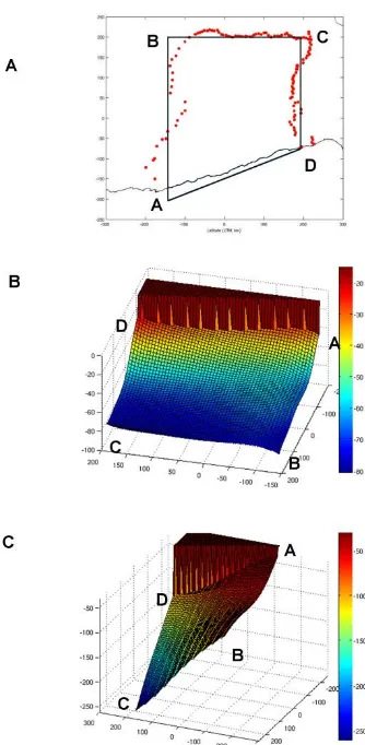
Figure 3.10 Moho and slab models in 3D ... 67
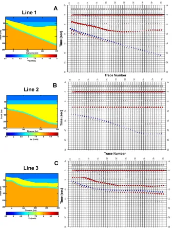
Figure 3.11 Comparison of FD models and synthetics for all arrays ... 69
Figure 3.12 Comparison of normal and flat slab images ... 71
Figure 3.13 Seismicity and elevation comparison, Flat/Normal subduction regions ... 73
Figure 4.1 Station installation ... 86
Figure 4.2 Data from the Sandwich Islands on 12/08/2010 ... 87
Figure 4.3 Processing methods, filtering ... 89
Figure 4.4 One versus two second filtered receiver functions ... 91
Figure 4.5 Time versus frequency domain deconvolution, line 3 ... 94
Figure 4.6 Time versus frequency domain from CCP stacks ... 95
Figure 4.7 Time versus frequency domain receiver functions for 12/08/2010 ... 97
Figure 4.8 PG40 time and frequency domain deconvolution ... 98
Figure 4.9 PG50 frequency versus time domain deconvolution ... 99
Figure 4.10 PE46 receiver functions, all phases (P, PP, and PKP) ... 101
Figure 4.11 Comparison of P/PP images with PKP for Line 1 ... 103
Figure 4.12 S wave RFs, Line 1 ... 105
Figure 4.14 Radial and transverse receiver functions for PF25 ... 109
Figure 4.15 Radial and transverse receiver functions for PF37 ... 110
Figure 4.16 Transverse RF stacks for PF25 from different azimuthal directions ... 111
Figure 4.17 Transverse RF stacks from the NW and SE for PF42 ... 112
Figure 4.18 Stations PF42 and PF43 axis of symmetry in transverse RFs ... 113
Figure 4.19 Stations PF29 and PF31 symmetry axis ... 114
Figure 4.20 Stations PF23 and PF24 symmetry axis ... 115
Figure 4.21 Stations PF12 and PF13 symmetry axis ... 116
Figure 4.22 CCP stacks from each azimuthal direction for Line 3 ... 1177
Figure 4.23 Backprojection for station PE46 ... 119
Figure 4.24 Image for Line 1 based on CCP stacks ... 120
Figure 4.25 Large earthquakes near arrays during time of array operation ... 124
Figure 4.26 Deep events which can be used for local receiver functions ... 125
Figure 4.27 Processing of local receiver function on 11/22/2011 ... 127
Figure 4.28 Local RF bandpassed to 2 sec. for Line 1, 2011/11/22 ... 128
Figure 4.29 Local RF, 2011/11/22, bandpassed to 2 Hz ... 129
Figure 4.30 Large and deep events used for analysis of pP and sS precursors ... 130
Figure 4.31 Precursor to pP phase from 08/26/2008 event in N. Peru ... 132
Figure 4.32 Stack to find precursors to sS phase for event on 07/12/2009. ... 133
Figure 4.33 More checks for pP precursors in Peru events ... 134
Figure 4.34 Data from 7/12/2009 bandpassed to 1 and 10 sec... 135
Figure 4.35 Data from 9/05/2009 bandpassed to 1 and 10 sec... 136
Figure 4.36 Data from 9/30/2009 bandpassed to 1 and 10 sec... 137
Figure 4.37 Structural models for southern Peru ... 138
Figure 4.38 Finite difference synthetics for 2009/07/12 . ... 140
Figure 4.39 Finite difference synthetics for 2009/09/05 . ... 141
Figure 4.40 Finite difference synthetics for 2009/09/30 . ... 142
Figure 4.41 CMT solutions for 10/28/2011 ... 1444
Figure A.1 PKP receiver functions ... 152
Figure A.2 P wave velocity models ... 153
Figure A.3 PKP versus P/PP slab ... 154
Figure A.4 Synthetic RF image ... 155
Figure A.5 Brazilian Shield/Line 1 model ... 156
Figure A.6 Initial model of Sheild... 156
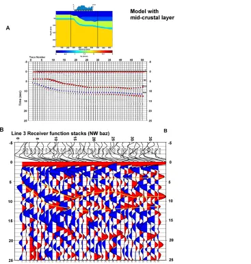
Figure B.1 Midcrustal signal ... 157
Figure B.2 Different slab models for Line 2 ... 158
Figure B.3 Seismicity across Nazca Ridge ... 159
Figure B.4 Migrated images of Lines 1 and 3, interpreted ... 161
Figure B.5 RF migrations of Lines 1 and 3, uninterpreted ... 162
Figure C.1 The team ... 163
Figure C.2 Obtaining wireless connectivity ... 164
Figure C.3 Wireless links between sites ... 165
Figure C.4 Installation procedure ... 166
Figure C.5 Field challenges ... 167
Figure C.7 PF11 Transverse RFs, stacks from NE/SW and NW/SE ... 169
Figure C.8 Transverse RFs for PF12 ... 170
Figure C.9 Transverse RFs for PF12, stacks/average for NW/SE ... 171
Figure C.10 Transverse RFs for PF13... 172
Figure C.11 Transverse RFs for PF13, stacks/average for NE/SW ... 173
Figure C.12 Transverse RFs for PF23... 174
Figure C.13 Transverse RFs for PF24... 175
Figure C.14 Transverse RFs for PF29... 176
Figure C.15 Transverse RFs for PF37... 177
Figure C.16 Transverse RFs for PF37, stacks/averages for NE/SW and NW/SE ... 178
Figure C.17 Transverse RFs for PF39... 179
Figure C.18 Transverse RFs for PF06... 180
Figure C.19 Transverse RFs for PF07... 181
Figure C.20 Radial and transverse RFs for PG27 ... 182
Figure C.21 Radial and transverse RFs for PG40 ... 183
Figure C.22 Radial and transverse RFs for PG42 ... 184
Figure C.23 Figure 4.28, no interpretive lines . ... 185
NOMENCLATURE
Subduction. Describes the movement of two tectonic plates in which a denser plate is forced beneath the lithosphere of a less dense plate
Normal subduction. Subduction in which the descending plate subducts at an intermediate angle close to 30 degrees.
Flat slab subduction. Subduction in which the descending plate subducts at a very shallow angle of less than 10 degrees for a portion of the subduction length. For example a plate which initially starts off subducting at a steep angle near the trench but flattens out to subduct almost horizontally beneath the overriding plate for a distance of several hundred kilometers before resuming
subduction at a steeper dip angle would be considered flat slab subduction.
Underthrusting. A process during compression in which one rock body is thrust beneath another relatively stable rock structure.
Shield. Typically refers to exposed precambian igneous and metamorphic rocks that form the stable interior of the continent
Moho. Short for Mohorovičić Discontinuity, the boundary between the crust and mantle marked
by a seismic velocity increase
Chapter 1: Introduction and Summary
The following chapters provide details of the methods, analysis, results, and discussion of
seismic data collected by arrays of seismic stations installed in southern Peru. Each
chapter is structured as a self-contained paper and will have its own set of references at
the end. The second chapter is in press with Journal of Geophysical Research-Solid
Earth, while the third chapter was recently submitted to Geophysical Journal
International.
The subduction style of the Nazca plate beneath South America varies along strike from
areas of “normal subduction” where the slab dips at angles around 25˚-30˚, to areas of flat slab subduction where the Nazca plate subducts at an angle less than 10˚ beneath South
America, as observed from seismicity in the Wadati-Benioff zone. Areas of normal
subduction include southern Ecuador (~0˚-2˚ S), southern Peru/northern Chile (~ 15˚-27˚ S), and southern Chile (~33˚-45˚ S). Areas of flat slab subduction include central and
northern Peru (2˚-15˚ S), central Chile (~27˚-33˚ S) and central Ecuador (0˚-2˚ N)
(Barazangi and Isacks 1976). Southern Peru represents a transition from normal to flat
slab subduction. Three seismic arrays were arranged roughly in the shape of a box to
sample the region of normal subduction (perpendicular to the trench), transition from
normal to flat slab subduction (parallel to the trench), and region of flat slab subduction
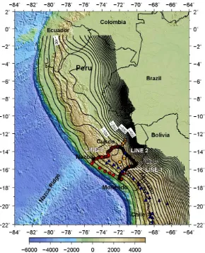
Figure 1.1. Topography and bathymetry map of Peru showing slab contours from the Slab 1.0 model. The seismic arrays are shown as red circles. Orange circles denote added stations from the CAUGHT/PULSE experiments. Dormant/active volcanoes are shown as blue/yellow triangles.
The purpose of the project is to clarify the structure beneath the arrays to learn more
about the present state of the subduction system, compare the normal and flat slab
regions, and study the nature of the transition between the two subduction regimes.
Overarching questions which stem from these observables are what are primary causes of
The array in the flat slab region is located near where the Nazca Ridge is presently
subducting and can be useful in estimating the effect of the ridge on the subduction
system. The thickened crust from subducting oceanic ridges, plateaus, and other such
impactors has been suggested to be a possible cause or contributor to flat slab subduction
by adding to the buoyancy of the subducting plate (Gutscher, Olivet, et al. 1999;
Gutscher, Malavielle, et al. 1999, Gutscher et al. 2000; van Hunen et al. 2002a, 2002b,
2004; McGeary et al. 1985, and Rosenbaum and Mo 2011). This notion is supported by
observations that many flat slab regions have corresponding buoyant impactors such and
the Juan Fernandez ridge in Chile and the Carnegie Ridge in Ecuador. A difference
between Peru and other flat slab regions is that the flat slab region in Peru is over 1500
km in length which is about three times the length of many other flat slab regions. The
Nazca Ridge has been migrating south through time and is located near the southern end
of the flat slab region but is not expected to have enough buoyancy to support the length
of the flat slab region or keep the slab from returning to a normal dip angle in its wake.
The array in the normal subduction region intersects the present active volcanic arc which
ends at the southern end of the flat segment where there is a volcanic gap. Gaps in
volcanism are observable in many flat slab regions because the lack of asthenospheric
wedge between the subducting and overlying plates inhibits partial melting (Gutcher,
Malavielle, et al. 1999). A look at the migration of the volcanic arc through time
provides information about the tectonic evolution of a region. For example when a
steeply dipping slab begins to flatten, the arc is seen to advance or migrate inland away
2005; Kay and Mpodozis 2002). As a flat slab begins to steepen again (or “roll back”),
the volcanic arc is seen to move toward the trench which is thought to be happening in
Mexico (Ferrari et al, 2001). In some areas both processes can be observed as the
volcanic arc first migrates away from the trench and later migrates back to the trench as
happened in western North America during the Laramide (Saleeby 2003). In Peru the
volcanic arc was observed to move eastward before extinguishing (Soler and Bonhomme,
1990) and over time as the slab begins to steepen due to eclogitization and increasing pull
from the already subducted material the arc will begin to migrate westward again.
The second chapter in this work presents results from “Line 1” running from Mollendo to
Juliaca in the normal slab region where the slab is seen to be dipping at 30 degrees. The
receiver function method is used to provide direct information about the structure beneath
the stations. Signals are observed from the Moho at the base of the crust and the top of
the subducting Nazca plate. One of the key observations is of a strong midcrustal
positive impedance signal at 40 km depth beneath the eastern portion of the array where
the Moho depth is observed to be around 70-75 km beneath the Altiplano. This is
suggested to be a possible observation of the underthrusting of the Brazilian Shield which
other authors have suggested underthrusts as far as the Eastern Cordillera (McQuarrie et
al. 2005; Gubbels et al. 1993; Lamb and Hoke 1997; Beck and Zandt 2002). We suggest
here that it underthrusts farther beneath southern Peru and even underlies a portion of the
Altiplano. Such an observation has implications for the timing of uplift in the Altiplano.
We suggest that the underthrusting of the Brazilian shield is more consistent with a
gradual uplift model over the last 40 Ma rather than rapid uplift over the past 10 Ma
have occurred further south in the Andes in the Puna Plateau, we suggest that the
dominant mechanisms for uplift in the Altiplano of southern Peru are crustal shortening
accompanied by tectonic underthrusting from the Brazilian craton.
The third chapter presents results from “Line 2” and “Line 3” in the transition from
normal to flat slab subduction and flat slab regions respectively. Line 2 shows the
clearest signal from the midcrustal structure at 40 km depth. The shape of the slab is
observed and is suggested to be a contortion rather than a tear in the slab. Results from
Line 3 show the slab flattening out almost horizontally beneath the Altiplano at a depth of
about 100 km. Results from this array are compared to the results from Line 1 in the
normal subduction region.
The fourth chapter presents further details of the methods used including methods which
are not presented in the papers. The results from this project are part of the PeruSE (Peru
Seismic Experiment) which began with field work and installation of broadband seismic
stations in 2008. The details of installation and seismic equipment used are presented.
The second array was installed and began collecting data in late 2009 while half of the
third array began collecting data in late 2010. The installation of the third array was
completed in 2011. After the collection of seismic data, teleseismic events were
analyzed with distances greater than 30 degrees and magnitudes greater than 5.8. The
receiver function method was used to provide more information about the structure
beneath the stations using deconvolution in the frequency domain. Both these results and
results using iterative time domain deconvolution are described. Although most receiver
great distance of many events from Peru made it useful to be able to include PP and PKP
phases. Results are compared using the various P-based phases to show the compatibility
of the receiver functions using the different phases. In addition to P, PP, and PKP phases,
S wave receiver functions were also attempted which have been used to look for the
lithosphere-asthenosphere boundary (LAB). Multiple receiver functions for each station
from similar azimuthal directions are stacked to obtain estimates for Moho depth and
Vp/Vs from the maximum summation of receiver functions at the time of the converted
phase and multiples. Although most of the analysis is done with radial receiver function,
transverse receiver functions were also analyzed. The presence of energy on the
transverse component can be suggestive of either a dipping interface or anisotropy. The
structure beneath the stations, including interfaces such as the Moho and subducting
oceanic crust can be clarified by plotting the amplitudes of receiver functions in cross
section using methods such as backprojecting rays and CCP (common conversion point
stacking). The backprojection method assumes an approximately linear ray path and
plots the amplitudes of receiver functions from the direction in which the energy arrived
so that each point along the receiver function is at the correct depth and distance from the
station. The amplitude at any given point in the image is an average of the amplitudes of
receiver functions which pass through that point. The CCP method is similar except it
calculates the piercing point of the ray with the expected depth of the Moho. All other
rays which pass through this region are stacked and the resulting stacks are plotted. The
receiver function methods use an average P wave velocity model. Simple 2D velocity
models are tested using finite difference modeling. Two different methods are used to
events allowing for the comparison of synthetic seismograms with data. Local events
were also analyzed but further analysis of local earthquakes is an area for future study.
In summary, the receiver function results shown in these chapters clarify the structure
beneath southern Peru to elucidate the present state of the subduction system. Results are
compared for the normal and flat slab regions which has implications for studying the
causes of flat slab subduction. The transition from normal to flat slab subduction is also
observed.
Chapter 1 References
∙ Barazangi, M., and B. L. Isacks (1976), Spatial distribution of earthquakes and
subduction of the Nazca plate beneath South America, Geology, 4, 686–692.
∙ Beck, S., and G. Zandt (2002), The nature of orogenic crust in the Central Andes,
Journal of Geophysical Research, 107, 2230.
∙ Ferrari, L., C. M. Petrone, and L. Francalanci (2001), Generation of oceanic-island
basalt-type volcanism in the western Trans-Mexican volcanic belt by slab rollback,
asthenosphere infiltration, and variable flux melting, Geology, 29 (6), 507-510.
∙ Gubbels, T., B. Isacks, and E. Farrar (1993), High-level surfaces, plateau uplift, and
foreland development, Bolivian central Andes, Geology, 21, 695–698.
∙ Gutscher, M., J. Malavielle, S. Lallemand, J.-Y. Collot (1999), Tectonic segmentation
of the North Andean margin: Impact of the Carnegie Ridge collision, Earth and
Planetary Science Letters 168, 255–270.
∙ Gutscher, M., J. Olivet, D. Aslanian, J. Eissen, and R. Maury (1999), The “lost Inca
171 (3), 335–341.
∙ Gutscher, M., W. Spakman, H. Bijwaard, and E. Engdahl (2000), Geodynamics of flat
subduction: Seismicity and tomographic constraints from the Andean margin,
Tectonics, 19 (5), 814–833.
∙ Haschke M. (2002), Evolutionary geochemical patterns of Late Cretaceous to Eocene
arc magmatic rocks in North Chile: implications for Archean crustal growth, EGU
Stephan Mueller Special Publication Series, 2, 207–218.
∙ Kay, S. M. & J. M. Abbruzzi (1996), Magmatic evidence for Neogene lithospheric
evolution of the central Andean “flat-slab” between 30˚ S and 32˚ S, Tectonophysics,
259, 15–28.
∙ Kay, S. M., E. Godoy, & A. Kurtz (2005), Episodic arc migration, crustal thickening,
subduction erosion, and magmatism in the south-central Andes, GSA Bulletin, 117,
(1/2), 67–88.
∙ Kay, S. M. & C. Mpodozis (2002), Magmatism as a probe to the Neogene shallowing of
the Nazca plate beneath the modern Chilean flat-slab, Journal of South American
Earth Sciences, 15, 39–57.
∙ Lamb, S., and L. Hoke (1997), Origin of the high plateau in the Central Andes, Bolivia,
South America, Tectonics, 16 (4), 623–649.
∙ McGeary S., A. Nur, and Z. Ben-Avraham (1985), Spatial gaps in arc volcanism: the
effect of collision or subduction of oceanic plateaus, Tectonophysics, 119, 195–221.
∙ McQuarrie, N., B. Horton, G. Zandt, S. Beck, and P. DeCelles (2005), Lithospheric
evolution of the Andean fold-thrust belt, Bolivia, and the origin of the central
∙ Rosenbaum, G., and W. Mo (2011), Tectonic and magmatic responses to the subduction
of high bathymetric relief, Gondwana Research, 19, 571–582.
∙ Saleeby, J. (2003), Segmentation of the Laramide Slab–evidence from the southern
Sierra Nevada region, GSA Bulletin, 115, 6, 655–668.
∙ Soler, P. & M. Bonhomme (1990), Relation of magmatic activity to plate dynamics in
central Peru from Late Cretaceous to present, Geological Society of America, Special
paper 241.
∙ van Hunen, J., A. van den Berg, and N. Vlaar (2002a), The impact of the South
American plate motion and the Nazca Ridge subduction on the flat subduction below
South Peru, Geophysical Research Letters, 29 (14).
∙ van Hunen, J., A. van den Berg, and N. Vlaar (2002b), On the role of subducting
oceanic plateaus in the development of shallow flat subduction, Tectonophysics, 352,
317–333.
∙ van Hunen, J., A. van den Berg, N. Vlaar (2004), Various mechanisms to induce
present-day shallow flat subduction and implications for the younger Earth: a
numerical parameter study, Physics of the Earth and Planetary Interiors , 146, 179–
Chapter 2: Normal Subduction Region
Structure of the Subduction System in Southern Peru
from Seismic Array Data
1
Kristin Phillips, 1Robert W Clayton, 2Paul Davis, 4Hernando Tavera, 2Richard Guy,
1
Steven Skinner, 2Igor Stubailo, 3Laurence Audin, 4Victor Aguilar
1
Caltech Seismological Laboratory, Pasadena CA, United States
2
UCLA Center for Embedded Networked Sensing, UCLA, Los Angeles, CA, United States
3
IRD, Casilla 18-1209, Lima 18, Peru
4
Instituto Geofisico del Peru, Lima, Lima 100, Peru
Abstract
The subduction zone in southern Peru is imaged using converted phases from
teleseismic P, PP, and PKP waves and P wave tomography using local and teleseismic
events with a linear array of 50 broadband seismic stations spanning 300 km from the
coast to near Lake Titicaca. The slab dips at 30 degrees and can be observed to a depth
of over 200 km. The Moho is seen as a continuous interface along the profile and the
crustal thickness in the back-arc region (the Altiplano) is 75 km thick, which is
sufficient to isostatically support the Andes, as evidenced by the gravity. The shallow
crust has zones of negative impedance at a depth of 20 km, which is likely the result of
positive impedance contrast, which we interpret as the western extent of the Brazilian
Craton as it underthrusts to the west. The Vp/Vs ratios estimated from receiver
function stacks show average values for this region witha few areas of elevated Vp/Vs
near the volcanic arc, and at a few points in the Altiplano. The results support a model
of crustal thickening in which the margin crust is underthrust by the Brazilian Shield.
2.1. Introduction
The subduction of the Nazca plate in southern Peru represents a transition region from a
shallow-dip system in northern and central Peru to normal-dip in southern Peru
(Barazangi and Isacks, 1976; Norabuena et al., 1994). Similar alternating sequences
are representative of the subduction of the Nazca plate beneath South America, which
have evolved with time (Ramos, 2009). The flattening of the slab in northern and
central Peru has been proposed to be due the subduction of the Nazca Ridge (Gutscher
et al., 2000) which has been sweeping southward over the past 10 Myr due to its
oblique subduction direction. The subduction angle between the Nazca and South
American plates is about 77 degrees resulting in a normal component of subduction of
6.1 cm/yr and tangential velocity of 4.3 cm/yr (Hampel, 2002). The slab has been
progressively flattening in the wake of this feature, and its present configuration is
shown in figure 2.1, which shows the depth contours of the slab. Also shown is the
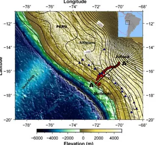
Figure 2.1. Topography and bathymetry of Peru showing the location of the subducting Nazca Ridge and the Altiplano of the central Andes. Variations in the dip angle of the Nazca plate can be seen through a contour model based on fits to seismicity. The locations of seismic stations installed in Peru as part of this study are denoted by red circles. The black line A-A’ shows the location of the cross section plotted in Figure 2. Active and dormant volcanoes are denoted by blue and white triangles. The volcanic arc is located in the region of normal subduction dip angle in southern Peru while a volcanic gap is observable in the flat subduction regime in central and northern Peru.
In this chapter, we focus on the region of normal-dip subduction south of Nazca Ridge
that we assume represents the subduction system before the flattening process.
According to Ramos (2009) this region has experienced uninterrupted normal
slab suggests that this zone has a natural cycle of normal/shallow subduction that is
driven by lithospheric delamination (DeCelles et al., 2009). This process is also
proposed as the cause of the rapid rise of the Andes in the last 10 Ma
(Gregory-Wodzicki, 2000; Garzione et al, 2006, 2008; Ghosh et al., 2006), however, more recent
studies now propose the rise was a continuous process over the last 40 Ma., thus
obviating the need of a rapid process such as delamination (Barnes and Ehlers, 2009;
Ehlers and Poulsen, 2009; McQuarrie et al., 2005; Elger et al., 2005; Oncken et al.,
2006). Results from this study support underthrusting of the Brazilian shield beneath
Peru (McQuarrie et al., 2005; Allmendinger and Gubbels, 1996; Horton et al., 2001;
Gubbels et al., 1993; Lamb & Hoke, 1997; Beck & Zandt, 2002), which is more
consistent with a gradual uplift model for this section of the Altiplano. The
eclogitization which would occur in the case of delamination needs a significant
amount of water (Ahrens & Shubert, 1975; Hacker, 1996), which is not present in the
Brazilian shield crust (Sighinolfi, 1971). Low silicic content also supports
eclogitization since the water content of hydrous minerals increases with decreasing
silica and increasing alumina (Tassara, 2006). Both argue that the granulites of the
lower Brazilian shield (Sighinolfi, 1971) would be stable as we find here.
To image the subduction zone, a linear array of 50 stations was deployed perpendicular
to the subduction trench for a distance of 300 km, with an average interstation spacing
of 6 km. This configuration was chosen to provide an unaliased image of the system
from the lower crust to the slab. The slab dip is well defined by seismicity down to a
depth of 250 km where there is a gap in seismicity. Cross sections and event locations
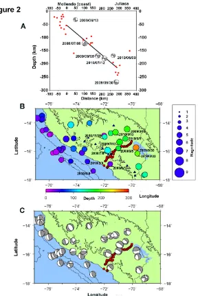
Figure 2.2. (A) Seismicity cross section along the seismic array. Hypocenters projected along the trend of the array are located within 60 km of the line. Earthquakes are from the EHB catalog (Engdahl et al. 1998; Engdahl & Villaseñor 2002) and are of
magnitudes of 5.0 or greater. The black line is the location of the slab from receiver functions. Also shown are the focal mechanisms for several events near the line from the Harvard CMT dataset. (B) Locations of local earthquakes, as located by the Instituto Geofisico del Peru (IGP), which have occurred since the installation of the seismic arrays in Southern Peru. Small red circles denote the location of seismic stations. The size of the circles representing earthquake locations is scaled by
In this study, we present a detailed image of the slab and lithosphere based on receiver
functions and tomography that establishes the basic structure and properties of the
normal-dipping part of the subduction in this region.
2.2 Data, Methods, and Results
2.2.1 Receiver Functions
The analysis in this paper is based on over two years of data (June 2008 to August
2010) recorded on the array shown in figure 2.1. The receiver functions utilize phases
from teleseismic earthquakes with distance-magnitude windows designed to produce
satisfactory signal to noise with minimal interference by other phases. The phases and
their windows are: P-waves (>5.8 Mw, 30–90 degrees), PP-waves (>6.0 Mw, 90–180
degrees) and PKP waves (>6.4 Mw, 143–180 degrees). In total there were 69 P-phases,
Figure 2.3. Location of events used in this study. (A) Teleseismic events between 30 and 90 degrees distance from Peru were used to make P-wave receiver functions. (B) Events greater than 90 degrees from Peru. The more distant events were used for studying converted arrivals of PP or PKP phases.
PKP phases were used because of the large number of useable events that are greater
than 90 degrees from Peru (figure 2.3). Due to the almost vertical arrival angle of these
phases, no conversion is expected at horizontal interfaces such as the Moho, however
PKP phases are useful for imaging dipping interfaces such as the slab. Events were
selected according to signal quality after bandpass filtering from 0.01 to 1 Hz. Similar,
but less resolved results were obtained for a 0.01 – 0.5 Hz passband. An example of
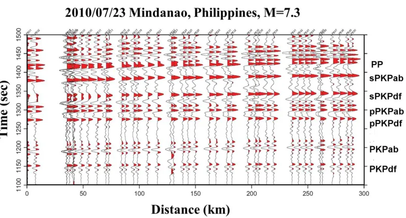
Figure 2.4. Seismic data measured by the array from the magnitude 7.3 earthquake in the Philippines which occurred on July 23, 2010. This section of the seismogram includes arrivals of PKP phases. Some phases are identified on the right of the record section. The distance axis represents distance from a reference point near the end of the seismic line closest to Mollendo on the coast and the time axis gives time after the origin time of the event. The bandpass filter used is from 0.01 to 1 Hz. See supplemental material for an example of a receiver function using the PKP phase.
Receiver functions are constructed by the standard method described in Langston
(1979) and Yan and Clayton (2007). Source complexities and mantle propagation
effects are minimized by deconvolving the radial component with the vertical.
Frequency-domain deconvolution (Langston, 1979; Ammon, 1991) was used, with a
water level cutoff and Gaussian filter applied for stability. A time window of 120
seconds, a water level parameter of 0.01 and Gaussian filter width of 5 seconds were
used during the deconvolution process. The processing of PKP receiver functions was
similar to P and PP phases with the same factors used for deconvolution. Both PKPab
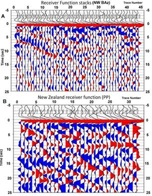
in figure 2.5, which shows stacked RFs from a NW azimuth to Peru, as well as a single
event occurring in New Zealand using the PP phase for comparison.
Figure 2.5. (A) The top set of receiver functions shows a stack for each station from events located at a northwest back azimuth from Peru. (B) The bottom receiver
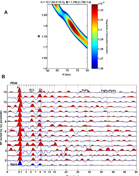
RFs are stacked using the method of Zhu and Kanamori (2000) which uses the
converted phase and multiples to obtain estimates of the depth of an interface and
average Vp/Vs ratio above the interface by summing along moveouts of the converted
phases as a function of ray parameter (Zhu and Kanamori, 2000). A search is done
over a range of depths and Vp/Vs ratios based on stacks of many events from similar
backazimuths. Figure 2.6 shows an example of stacking and grid search for individual
stations. Uncertainty estimates are based on the 95 percent confidence interval.
A simple migrated image is then constructed by backprojecting the receiver functions
along their ray paths. The angle from the station is estimated using the ray parameter
and event backazimuth, with corrections for the station elevation. A simple layered
velocity model based on IASP91 was used to backproject the rays. This approximation
was checked by comparison with other velocity models based on tomography and a
thicker crust but the migrated images were found to have Moho depths similar to the
results presented here.
2.2.1.1 Receiver Function Results
An image based on teleseismic P and PP receiver functions produced from data
recorded by the seismic array with events from all azimuths is shown in figure 2.7. The
Moho has an initial depth of around 25 km near the coast and deepens to around 75 km
depth beneath the Altiplano. Also evident is a positive impedance midcrustal signal at
Figure 2.7. (A) Depth versus distance cross sectional image from Line 1 based on teleseismic P and PP receiver functions from all azimuthal directions showing the upper 120 km. Depth is the distance below mean sea level. (B) Same as in A showing
interpretations of the mid crustal structure (MC) and Moho as well as a signal from the slab.
The subducting slab can be clearly observed in figure 2.8, which is a stack of data from
the northwest azimuth. Receiver functions were stacked to obtain the depth of the
Moho by the method of Zhu and Kanamori (2000) as shown in figure 2.6, and the
resulting depth estimates are shown in figure 2.8, superimposed on the RF image. Also
shown are the crustal Vp/Vs ratios along the line, which have an average value of
around 1.75. There are three zones of elevated Vp/Vs ratios in the Altiplano, one of
which corresponds to the current arc. These are coincident with negative impedances
hence are likely related to magmatic processes. This identification is clearest for the
anomalies associated with the current arc. The other two may indicate the location of
focused magmatic activity in the past. Similar features were observed in northern Chile
(Leidig and Zandt, 2003; Zandt et al., 2003). The dense station spacing allows for an
unambiguous tracing of the Moho, slab, and midcrustal feature.
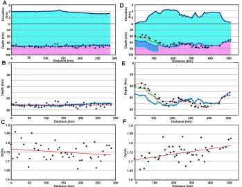
Vp/Vs values (y-axis) versus station number (proxy for distance). Orange shading represents high Vp/Vs values, green shading represents mid-range values, and light blue shading represents lower Vp/Vs values. The blue line shows the three-point running average of the Vp/Vs values. (D) Map of southern Peru showing a line with colors representing Vp/Vs ratios estimated from stacking of receiver functions. Black triangles represent active and dormant volcanoes in arc.
Receiver functions based on the PKP phase show a negative pulse corresponding to the
top of the oceanic crust of the descending slab closely followed by a positive pulse at
the transition to oceanic mantle. From the teleseismic P and PP phase receiver function
results, this double pulse seen in the slab is observed most strongly down to a depth of
around 100 kilometers. The receiver function images are consistent with the results of
Kawakatsu and Watada (2007), which suggests that this is related to the transport of
hydrous minerals in oceanic crust into the subduction zone. The transition between
these signals is consistent with the location of the subducting Nazca plate as described
by seismicity in the Wadati-Benioff zone (figure 2.9). The seismicity is centered near
the transition between the positive and negative pulses. Note a phase difference in the
slab signal between the PKP image and P/PP images due to a change in sign of the
converted phase because of the steep angle of incidence of incoming PKP waves (see
Figure 2.9. Backprojected receiver function image based on PKP receiver functions. Only the PKPdf branch is included in this image. All events used come from the Indonesian region. Images show a sharp, well defined boundary at the expected
location of the slab based on seismicity. Depth is the distance below mean sea level and distance is measured from the first station on the coast. Topography is shown above the image in blue.
2.2.1.2 Receiver Function Waveform Modeling
The receiver function images obtained above were checked using 2D finite-difference
waveform modeling (Kim et al. 2010). The 2D velocity model includes depth
information based on receiver function results and velocities consistent with averages
taken from Cunningham and Roecker (1986) for southern Peru, which we modified to
include a midcrustal layer contrast to model the positive-impedance feature. The more
recent model of Dorbath et al. (2008) was also tested and compared with the southern
Peru model (shown in the supplementary materials) and the results are similar to those
shown here. A simplified velocity model, which incorporates average values
underlying mantle was selected for modeling purposes. The model has dimensions of
500 km horizontal distance by 250 km depth. Synthetic receiver functions are produced
with P-wave plane waves with varying ray parameters imposed on the bottom and sides
of the model. Seismograms were produced with frequencies up to 1 Hz, and then
processed as RFs with the same techniques and parameters used with the real data. A
The synthetics, which incorporate midcrustal structure are observed to be consistent
with RF data and results as seen in figure 2.11. They show a positive signal at around 5
seconds (midcrustal), which is observed in the receiver functions as well as an observed
multiple that is not present in models without the midcrustal structure.
circles denote the depth of the Moho from synthetics. (B) Positive and negative pulses corresponding to the bottom and top of the oceanic crust of the slab as seen in FD synthetics are shown as magenta and yellow circles overlaying the PKP image from figure 2.10.
The velocity is then combined with a structural model derived from the receiver
functions and is tested with a deep local event that occurred beneath the array on the
slab interface (figure 2.12). The finite difference code is based on the one discussed in
Vidale et al. (1985). The event is Mb 6.0 and is located at a depth of 199 km and about
60 km off the line. The resultant synthetics from finite difference modeling have P
wave arrival characteristics and differential P to S wave travel times consistent with the
data. The synthetics and data also have a similar arrival caused by a conversion at the
Moho which provides confirmation of the Moho depth. An arrival due to phase
conversions at the midcrust can be seen in the synthetics and also appears to also be
present in the data, particularly towards the inland end of the seismic array suggesting
that the midcrustal structure does not underlie the entire seismic array in agreement
modeling. Shaded portions are extensions of the model to avoid artificial reflections. The location of the event at about 199km depth is shown by the pink circle. C) Data from a magnitude 6 event occurring on July 12, 2009 aligned by the P wave arrival (1). Time is on the x-axis and distance from coast is on the y-axis. D) Synthetics also aligned on the P wave arrival (1). The S wave arrival (2) can also be seen as well as signals from the Moho (3) and midcrustal interface (4). E) Comparison of data and synthetics near the P wave arrival where the synthetics are in red and the data is shown by the black line.
2.2.2 P-Wave Tomography
A total of 5677 travel–time residuals including 1674 teleseismic arrivals and 4003
local event arrivals were inverted to obtain the tomographic image shown in figure 2.13
using a 2D tomography program (Husker and Davis, 2009). The local events are
restricted to depths greater than 30 km, and with 125 km of the 2D line. The 2D
assumption appears justified by gravity based on gravity survey results (Fukao et al.
1989) and GRACE (Gravity Recovery and Climate Experiment) satellite data which
show little along-strike gravity variation indicating an approximately 2D crust, as well
as seismicity slab contours which show that the slab can also be considered
approximately 2D within about 100km of the array. The local earthquakes were first
located with an IASPEI (Kennett and Engdahl 1991) model that took into account the
changing Moho depth determined by receiver functions. A finite-difference program
was then used to relocate the events (Hole and Zeldt, 1995). The inversion consisted
of 680 20 km blocks (20x34) and was performed with damped least squares. In the
upper 350 km; the average number of hits/block was 142. The variance reduction was
Figure 2.13. Tomographic image beneath the seismic line using a 2D tomography code. In A) the results are percent slowness changes from the IASPEI model, and in B) the result is in absolute velocity. Locations of the Moho and top of the Slab from the receiver function study are plotted as white lines. Station locations are shown as black triangles and local earthquake locations used for tomography are shown as black circles. The image supports the model of a steeply dipping slab and thickened Moho.
The tomography results are presented in figure 2.13. Figure 2.13A shows perturbations
as percent deviations relative to the IASPEI starting model while figure 2.13B shows
through the station locations. For comparison, locations of the Moho and top of the
subducting slab from the receiver function analysis are superimposed on the figure and
show good agreement with the transitions in the image from low to higher velocities.
A standard checkerboard resolution test is shown in figure 2.14. The results are well
resolved in both the horizontal and vertical directions except at depth greater than 350
km on the northern end of the line.
2.3 Discussion
2.3.1 Crustal Thickness
Receiver function results for the normal subducting region of southern Peru show a
Moho that deepens from 25 km near the coast to a depth of around 75 km beneath the
Altiplano. Previous estimates of crustal thickness of the Altiplano are about 70-75 km
(Cunningham and Roeker, 1986; Beck et al., 1996; Zandt et al, 1994). McGlashan et al.
(2008) also estimated thicknesses from 59 to 70 in Southern Peru. The 75 km crust of
the Altiplano is approximately the thickness required for the region to be in Airy
Figure 2.15. Results from a gravity survey performed along the seismic array by Caltech and UCLA students during a geophysical field course. A) Observed absolute gravity (m/s2) B) Free air anomaly in mGal relative to the first station, which shows an increase near the start of the line due to uplift near the coast. (C) Topography along the array (D) Moho estimates from receiver function stacking and Moho depth estimates expected for Airy isostasy relative to a reference station.
One of the major processes which could contribute to this thickness is crustal
shortening. Gotberg et al. (2010) gave a preferred estimate of 123 km of shortening but
said that 240-300 km of shortening would be required for a 70 km thick crust. Other
suggested mechanisms for producing such a thickness include lower-crustal flow,
shortening hidden by the volcanic arc (Gotberg et al., 2010), thermal weakening
structure from tectonic events prior to orogeny (Allmendinger and Gubbels, 1996),
magmatic additions, lithospheric thinning, upper mantle hydration (Allmendinger et al.,
1997), plate kinematics (Oncken et al., 2006), shortening related to the Arica bend
(Kley & Monaldi, 1998; Gotberg et al, 2010), tectonic underplating (Allmendinger et
al, 1997; Kley & Monaldi, 1998), and other factors. The mechanism of tectonic
underthrusting is supported by our observations of a midcrustal structure and provides a
simple mechanism for explaining the crustal thickness in southern Peru.
2.3.2 Midcrustal Structure
The positive impedance structure observable at a depth of around 40 km is an unusual
crustal feature because the crust does not normally have an interface with a sharp
increase in velocity. One hypothesis that could explain this feature is underthrusting by
the Brazilian Craton. It is generally accepted that this underthrusting exists as far as the
Eastern Cordillera (McQuarrie et al., 2005; Gubbels et al., 1993; Lamb & Hoke, 1997;
Beck & Zandt, 2002). However the results presented here appear to support the idea
that it extends further to the west, as was suggested by Lamb and Hoke (1997). The
midcrustal signal at 40 km depth is observed continuously across multiple stations on
the eastern half of the array. The Conrad discontinuity, which is sometimes observed at
midcrustal depths of around 20 km was considered, but the processes involved in
crustal shortening and thickening are not expected to produce such a flat and strong
positive impedance feature at 40 km. The strength of the midcrustal signal relative to
the Moho signal (see figure 2.6), and the observation that the signal is limited to the
underthrusting as a more reasonable explanation. If the Brazilian craton underthrusts as
far as the Altiplano, it would substantially increase the thickness of the crust under the
Altiplano and hence affect the timing of the rise of the Andes. The rapid rise model of
Garzione et al. (2008), proposes a gradual rise of 2 km over approximately 30 Myrs,
followed by a rapid rise of 2 km over the last 10 Myrs. This is then used as evidence of
removal of the dense lower crust and/or lithospheric mantle (Ghosh et al. 2006) because
it is a process that can result in rapid uplift. An alternative model of the rise suggests
that the total rise proceeded gradually over 40 Myrs. This latter model is favored by the
midcrustal layer found in this study. The timing of underthrusting and nature of the
underthrusting Brazilian craton suggests that rather than eclogitization and
delamination of the lower crust and mantle lithosphere resulting in rapid uplift, the
process was more gradual. The underthrusting Brazilian craton would have removed
some of the preexisting lower crust and mantle lithosphere beneath the Altiplano and
replaced it with the Shield crust and underlying mantle lithosphere, thus contributing to
the crustal thickening observed beneath the Altiplano. Some of the uppermost crust of
the underthrusting Brazilian craton may have been eroded and deformed. The
remainder of the Shield crust is assumed to be denser than the upper Altiplano crust
resulting in higher seismic velocities. The lithosphere of the Brazilian craton is
suggested to taper off prior to the subducting Nazca plate as the subducting plate is
observed continuously to 250 km depth and is not impacted by the underthrusting
craton. The western limit of the underthrusting is not well defined in the images but it
does not appear to extend beyond the volcanic arc. The presence of the underthrusting
Comparing the model of evolution in Southern Peru with the overall evolution in the
central Andes, several authors (Allmendinger et al., 1997; Babeyko and Sobolev, 2005)
have suggested that there has been north–south variation in mechanisms and rates of
crustal thickening and uplift in the central Andes. The tectonic evolution in the
Altiplano may have differed from the uplift and evolution of the Puna plateau
(Allmendinger et al, 1997). Babeyko and Sobolov (2005) suggested that the type of
shortening (e.g., pure versus simple shear as discussed by Allmendinger and Gubbels,
1996) may be controlled by the strength of the foreland uppermost crust and
temperature of the foreland lithosphere. Hence, a weak crust and cool lithosphere in
the Altiplano could be supportive of underthrusting, simple shear shortening, and
gradual uplift while further south in the Puna the strong sediments and warm
lithosphere supports pure shear shortening, lithospheric delamination, and resultant
rapid uplift.
In addition to crustal information, receiver functions also show the subducting Nazca
plate dipping at an angle of about 30 degrees from both the P/PP and PKP phases for
Line 1. Figure 2.16 shows a cartoon interpretation of the array data. With the exception
of the midcrustal positive-impedance and its interpretation of underthrusting by the
Figure 2.16: Schematic model of receiver function images showing the underthrusting Brazilian shield (colored teal), light blue representing the upper crust, purple
representing the subducting oceanic crust, and green representing mantle. The small area of red represents a possible low velocity zone at around 20 km depth, which may correspond to magmatism.
Conclusions
Receiver function and tomographic studies using data from an array of 50 broadband
stations in Southern Peru image the region of normal subduction beneath the Altiplano.
Both approaches confirm previous estimates of Moho depth beneath the Altiplano
which reach a maximum value of about 75 km. The dipping slab is also clearly seen in
the images. A positive impedance midcrustal structure at about 40 km depth is seen in
the receiver functions indicating an increase in velocity in the lower crust. This feature
may be due to underthrusting of the Brazilian shield, previously believed to underlie the
Acknowledgements
We thank the Betty and Gordon Moore Foundation for their support through the
Tectonics Observatory at Caltech. This research was partially support by NSF award
EAR-1045683. Contribution number 199 from the Tectonics Observatory at Caltech.
Chapter 2 References
∙ Ahrens, T. J., and G. Schubert (1975). Gabbro-Eclogite reaction rate and its
geophysical significance, Reviews of Geophysics and Space Physics, 13 (2), 383-400
∙ Allmendinger, R., and T. Gubbels (1996), Pure and simple shear plateau uplift,
Altiplano-Puna, Argentina and Bolivia, Tectonophysics, 259, 1–13.
∙ Allmendinger, R., T. Jordan, S. Kay, and B. Isacks (1997), The e volution of the
Altiplano-Puna Plateau of the Central Andes, Annu. Rev. Earth Planet. Sci., 25,
139–174.
∙ Ammon, C., (1991), The isolation of receiver effects from teleseismic P waveforms,
Bull. Seismo. Soc. Am., 81, 6, 2504-2510.
∙ Babeyko, A., and S. Sobolev (2005), Quantifying different modes of the late
Cenozoic shortening in the central Andes, Geology, 33 (8), 621–624.
∙ Barazangi, M., and B. L. Isacks (1976), Spatial distribution of earthquakes and
subduction of the Nazca plate beneath South America, Geology, 4, 686–692.
∙ Barnes, J., and T. Ehlers (2009), End member models for Andean Plateau uplift,
Earth-Science Reviews, 97 (105-132).
∙ Beck, S., and G. Zandt (2002), The nature of orogenic crust in the Central Andes,
∙ Beck, S., G. Zandt, S. Myers, T. Wallace, P. Silver, and L. Drake (1996), Crustal-
thickness variations in the central Andes, Geology, 24 (5), 407–410.
∙ Cunningham, P., and S. Roecker (1986), Three-dimensional P and S Wave Velocity
Structures of Southern Peru and Their Tectonic Implications, J. of Geophys.
Res., 91 (B9), 9517–9532.
∙ DeCelles, P., and M. Ducea, P. Kapp and G. Zandt (2009), Cyclicity in Cordilleran
orogenic systems, Nature Geoscience, 2, pp 251-257, doi:10.1038/NGEO469.
∙ Dorbath, C., M. Gerbault, G. Carlier, and M. Guiraud (2008), Double seismic zone of
the Nazca plate in Northern Chile: High-resolution velocity structure, petrological
implications, and thermomechanical modeling, Geochemistry, Geophysics,
Geosystems, 9 (7), Q07, 2006.
∙ Ehlers, T., and C. Poulsen (2009), Influence of Andean uplift on climate and
paleoaltimetry estimates, Earth and Planetary Science Letters, 281, 238–248.
∙ Elger, K., O. Oncken, and J. Glodny (2005), Plateau-style accumulation of
deformation: Southern Altiplano, Tectonics, 24 (TC4020).
∙ Engdahl, E. R., R. van der Hilst, and R. Buland (1998), Global teleseismic earthquake
relocation with improved travel times and procedures for depth determination, Bull.
Seism. Soc. Am. 88, 722-743
∙ Engdahl, E. R. and A. Villaseñor (2002), Global Seismicity: 1900-1999, in W.H.K.
Lee, H. Kanamori, P. C. Jennings, and C. Kisslinger (editors), International
Handbook of Earthquake and Engineering Seismology, Part A, Chapter 41, 665-690
∙ Fukao, Y., A. Yamamoto, and M. Kono (1989), Gravity anomaly across the Peruvian
∙ Garzione, C., P. Molnar, J. Libarkin, and B. MacFadden (2006), Rapid late Miocene
rise of the Bolivian Altiplano: Evidence for removal of mantle lithosphere, Earth
and Planetary Science Letters, 241, 543–556.
∙ Garzione, C., G. Hoke, J. Libarkin, S. Withers, B. MacFadden, J. Eiler, P. Ghosh, and
A. Mulch (2008), Rise of the Andes, Science, 320, 1304–1307.
∙ Ghosh, P., C. Garzione, and J. Eiler (2006), Rapid uplift of the Altiplano revealed
through 13C-18O bonds in paleosol carbonates, Science, 311, 511–515.
∙ Gotberg, N., N. McQuarrie, and V. Caillaux (2010), Comparison of crustal thickening
budget and shortening estimates in southern Peru (12˚–14˚ S): Implications for
mass balance and rotations in the “Bolivian orocline”, GSA Bulletin, 122 (5–6), 727–
742.
∙ Gregory-Wodzicki, K. (2000), Uplift history of the Central and Northern Andes; a
review, GSA Bulletin, 112 (7), 1091–1105.
∙ Gubbels, T., B. Isacks, and E. Farrar (1993), High-level surfaces, plateau uplift, and
foreland development, Bolivian central Andes, Geology, 21, 695–698.
∙ Gutscher, M., W. Spakman, H. Bijwaard, and E. Engdahl (2000), Geodynamics of flat
subduction: Seismicity and tomographic constraints from the Andean margin,
Tectonics, 19 (5), 814–833.
∙ Hacker, B.R. (1996), Eclogite formation and the rheology, buoyancy, seismicity, and
H2O content of oceanic crust, AGU Monograph, p337-346.
∙ Hampel, A. (2002), The migration history of the Nazca Ridge along the Peruvian
active margin: a re-evaluation, Earth and Planetary Science Letters, 203, 665–679.
Geophys. J. Int., 121, 427-434.
∙ Horton, B., B. Hampton, and G. Waanders (2001), Paleogene synorogenic
sedimentation in the Altiplano Plateau and implications for initial mountain building
in the Central Andes, GSA Bulletin, 113, 1387–1400.
∙ Husker, A. and P. M. Davis (2009), Tomography and thermal state of the Cocos
plate subduction beneath Mexico City, J. Geophys. Res., 114, B04306.
∙ Isacks, B. (1988), Uplift of the Central Andean Plateau and bending of the Bolivian
Orocline, J. of Geophys. Res., 93 (B4), 3211–3231.
∙ Kawakatsu, H., and S. Watada (2007), Seismic evidence for deep-water
transportation in the mantle, Science, 316, 1468-1471.
∙ Kennett, B. L. N., and E. R. Engdahl (1991), Traveltimes for global earthquake
location and phase identification, Geophys. J. Int., 105, 429-465.
∙ Kim, Y., R. W. Clayton, and J. M. Jackson (2010), Geometry and seismic properties
of the subducting Cocos plate in central Mexico, J. Geophys. Res., 115, B06310.
∙ Kley, J. and C. R. Monaldi (1998), Tectonic shortening and crustal thickness in the
Central Andes: How good is the correlation? , Geology, 26, 8, 723-726.
∙ Lamb, S., and L. Hoke (1997), Origin of the high plateau in the Central Andes,
Bolivia, South America, Tectonics, 16 (4), 623–649.
∙ Langston, C. (1979), Structure under Mount Rainier, Washington, inferred from
teleseismic body waves, J. Geophys. Res., 84, 4749–4762.
∙ Leidig, M., and G. Zandt (2003), Modeling of highly anosotropic crust and application
to the Altiplano-Puna volcanic complex of the central Andes, J. Geophys. Res, 108
∙ McGlashan, M., L. Brown, and S. Kay (2008), Crustal thickness in the Central Andes
from teleseismically recorded depth phase precursors, Geophys. J. Int., 175, 1013-
1022.
∙ McQuarrie, N., B. Horton, G. Zandt, S. Beck, and P. DeCelles (2005), Lithospheric
evolution of the Andean fold-thrust belt, Bolivia, and the origin of the central
Andean plateau, Tectonophysics, 399, 15–37.
∙ Norabuena, E., J. Snoke, and D. James (1994), Structure of the subducting Nazca
Plate beneath Peru, J. Geophys. Res., 99, 9215–9226.
∙ Oncken, O., J. Kley, K. Elger, P. Victor, and K. Schemmann (2006), Deformation of
the Central Andean Upper Plate System-Facts, Fiction, and Constraints for Plateau
Models, Berlin, Springer, p. 569.
∙ Ramos, V. (2009), Anatomy and global context of the Andes: Main geologic features
and the Andean orogenic cycle, in Kay, S.M., Ramos, V.A., and Dickinson, W.R.,
eds., Backbone of the Americas: Shallow Subduction, Plateau Uplift, and Ridge and
Terrane Collision: Geological Society of America Memoir, 204, p31065,doi:
10.1139/2009.1204(02).
∙ Sighinolfi, G.P. (1971), Investigations into deep crustal levels: fractionating effects
and geochemical trends to high-grade metamorphism, Geochim. Cosmochim. Acta,
35, pp. 1005-1021.
∙ Tassara, A. (2006), Factors controlling the crustal density structure underneath active
continental margins with implications for their evolution, Geochem. Geophys,
Geosyst., 8, Q01001.
seismograms for SH-waves, Bull. Seismo. Soc. Am., 75, 6, 1765-1782.
∙ Yan, Z. and R.W. Clayton (2007), Regional mapping of the crustal structure in
southern California from receiver functions, J. of Geophys. Res., 112, B05311.
∙ Zandt, G., M. Leidig, J. Chmielowski, D. Baumont, and X. Yuan (2003), Seismic
detection and characterization of the Altiplano-Puna magma body, Central Andes,
Pure Appl. Geophys., 160, 789–807.
∙ Zandt, G., A. Velasco, and S. Beck (1994), Composition and thickness of the southern
Altiplano crust, Bolivia, Geology, 22, 1003–1006.
∙ Zhu, L., and H. Kanamori (2000), Moho depth variation in southern California from
Chapter 3: Subduction Transition and Flat Slab
Structure of the Subduction Transition Region from Seismic
Array Data in Southern Peru
Kristin Phillips and Robert W. Clayton
Abstract
Data from three seismic arrays installed in southern Peru was analyzed using receiver
functions from P, PP, and PKP wave phases, in order to image the subducted Nazca
slab. The arrays cover the transition region from flat slab subduction in central Peru to normal subduction with an angle of about 30˚ further south. The results provide an
image of the flattened slab from the coast to approximately 300 km inland and also
across the transition region from flat to 30-degree subduction, which appears to be a
bend rather than a tear in the slab. In the flat slab region, the slab is well defined near
the coast and flattens out at 100 km depth beneath the Altiplano. The slab appears to
start flattening some 400 km in advance of the subduction of the Nazca Ridge and the
flattening is maintained for 1300 km after its passage. The Moho begins at a depth of
around 30 km near the coast and has a maximum depth of 75 km beneath the Altiplano,
consistent with the results of the other arrays. The Vp/Vs ratios for both arrays exhibit
average values between 1.73 and 1.75 indicating that the region is most likely not
around 40 km depth, which is suggested to be a result of underthrusting of the Brazilian
shield. This would explain the missing crust needed to support the Altiplano.
3.1. Introduction
The dip of the subducted Nazca plate beneath southern Peru changes from shallow or
flat slab beneath central Peru to a steeper dip angle (“normal” subduction) of around 30
degrees beneath southern Peru. This transition is evident in the seismicity (Barazangi &
Isacks, 1976; Cahill and Isacks, 1992; Grange et al, 1984; Suarez et al, 1983), and by a
gap in the arc-volcanism (Gutsher, Olivet et al, 1999; Gutscher, Spakman et al. 2000;
McGeary et al, 1985). Adakitic magmas have also been associated with flat slab
regions (Gutscher, Maury, et al. 2000) and have been reported in southern
Ecuador/northern Peru (Beate et al, 2001). They are suggested to result from partial
melting of subducted oceanic crust (Gutscher, Maury, et al. 2000). Besides the
observed correspondence between adakites and flat slab regions, the partial melting
resulting in such magmas could also be a result of slab tearing at the transitions from
flat slab to a steeper dip angle (Yogodzinski et al, 2001). The lack of reported adakites
in southern Peru might indicate that the southern transition is slab bending rather than a
tear. The change in dip is coincident with the subduction of Nazca Ridge. This is one
of three zones of slab-dip changes along the western margin of Southern America. In
central Chile, the subduction of the Juan Fernandez Ridge is cited as the cause of the
flattening along its subduction trajectory (Pilger, 1981; Gutscher, Spakman et al, 2000;
flattening tightly conforms to the shape of the ridge. In Equador, the Carnegie Ridge
also apparently causes the slab to flatten (Gutscher,Malavielle et al. 1999).
Various mechanisms have been proposed as to the cause of flat slab subduction. Some
authors have noted a correlation between regions of flat slab subduction and the
presence of thickened oceanic crust such as that due to a subducting plateau or ridge
which could increase the buoyancy of the subducting slab (Gutscher, Maury et al.
2000). Gutscher et al. (1999) proposed that the length of flat subduction in Peru was
due to buoyancy effects resulting from two subducting ridges; the Nazca ridge and a
previously unknown impactor referred to as the Inca Plateau which is believed to be the
mirror image of the Marquesas plateau although recent plate movement reconstructions
call into question the proposed location and timing of the Inca plateau (Skinner and
Clayton 2012). Both plateaus were suggested to have formed at the Pacific-Farallon
spreading centre based on tectonic reconstructions. According to Hampel (2002), the
Nazca Ridge originally began subducting at 11˚S around 11.2 Ma. Since then it has
been sweeping south and presently has a migration rate of around 43 cm per year. The
area of flat subduction in Peru corresponds to the area swept out by the Nazca Ridge.
Thus the Nazca Ridge may have had an impact on the evolution and shape of the
subduction zone. In addition to buoyancy effects caused by a subducting ridge or
plateau, other factors could influence flat subduction such as the age of the lithosphere
being subducted (Sacks 1983), delay in the basalt to eclogite transformation (Gutscher,
Spakman et al. 2000; Pennington 1984), absolute motion of the upper plate (Olbertz et