By Machine Learning Techniques to
Estimate Wind Turbine Power Generation
Swarna Jain
Dept. of Computer ScienceBabulal Tarabai Institute of Research andTechnology, Sagar, India
Anil Pimpalapure
Assist. Proff (CSE)Babulal Tarabai Institute of Research and Technology Sagar, India.
ABSTRACT This paper provides an overview of the recent developments in machine learning techniques focused on prediction using regression. The machine learning techniques rapidly developed and regression techniques have been used for prediction. The wind turbine power curve shows the relationship between wind turbine power and wind speed. Wind turbine captures the wind speed and mechanical power produced is given to electric grids, hence wind speed has been taken into consideration for prediction of power. The main objective of this paper is to review and summarize the recent achievements in machine learning techniques, especially regression for prediction, thus providing a referee for study on related topics both from practical and academic points of view. This paper begins with power estimation techniques using mathematical formulae, their advantages and disadvantages. Then the methods based on power curve will be introduced. The recent development in the field of prediction using artificial neural networks is further. Introduced. The new trends of prediction are finally discussed.
Index Terms: -. Machine Learning, Power Curve, and wind turbine power curve.
1. Introduction
Increase in demand of renewable energy and clean source of energy for electricity generation and among all the renewable energy sources wind energy being most promising source of energy. Wind energy has potential to satisfy future electricity need. Wind Energy holds out a promising energy source but the uncertainties involved due to stochastic nature of wind accurate and reliable forecasting models are required to optimize the operation cost and improve the reliability of power system with increased penetration of mechanical power to electric grid [1][2][3]. Also by forecasting power one will be able expand the existing wind farms. In wind energy industry, the turbine power curve - a plot of generated power versus
ambient wind speed, is an important indicator of wind turbine performance. Power curve predicts power produced by turbine given wind speed, without the technical details of components of wind power generating system. A turbine manufacturer usually provides a nominal power curve as a reference. The actual power curve will vary from this nominal curve for a variety of reasons-some inherent to the incoming wind and its characteristics such as turbulence, some due to the way the turbine actually responds to the observed wind, but some may also be caused by multiple system faults - sensor and control faults, turbine or generator faults, etc.
[1][2]The minimum speed at which the turbine delivers useful power is known as the cut-in speed (uc). Rated speed (ur) is the wind speed at which the rated power, which is the maximum output power of the electrical generator, is obtained. The cut-out speed (us) is usually limited by engineering design and safety constraints. It is the maximum wind speed at which the turbine is allowed to produce power. The typical power curve is shown
in fig.1.
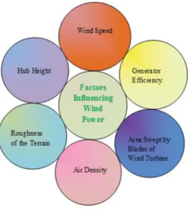
2. Factors Affecting Power Output
Wind speed, hub height, air density, area swept by blades of turbine, roughness of the terrain,
generator efficiency, turbine efficiency,
transmission system efficiency, temperature these are the factors affecting output power generated by wind turbine [2].
Given below is the equation specifying relationship between wind speed and height..
v2/ v1= (h2/ h1) (1)
Where,
v1, v2– wind velocity
h1, h2– height at which turbine is located
– ground friction coefficient
From this equation it is clear that wind speed is directly related to the height at which turbine is located.
More turbine efficiency, generator efficiency, transmission system efficiency promises more electric power.
Fig. 2: Factors affecting wind power.
Air density changes with change in value of altitude, temperature, and pressure and weather condition [15]. Atmospheric pressure decreases with height. So, power output on the high mountain gets reduced as compared to power output at sea level. Increase in wind speed gives maximum
power generated since wind speed is directly proportional to the power.
3. Models for Predicting Power Output
Fig. 3: Two broad categories of models for predicting power output.
3.1 Models Based On Fundamental Equation of Power Available in the Wind
The theoretical power captured by the rotor of a wind turbine (Pw) is given by
Pw= ½ ( AV3) W (2)
Ashok [Ashok 2007] presented that wind power output can be calculated as
Pe= t g(0.5) CpAv3 (3)
Variation in values of t , g and Cp with wind
speed and design of wind turbine, variation in value of air density with changing weather, variation in value of Pe for various wind speed ranges have not
been taken into consideration.
Nelson [Nelson 2006] evaluated average hourly wind speed data and converted it to wind turbine power and stated that
Pe(t) = ?? Av3(t)CpEffad (4)
Where, Effad is assumed as 95%
Variation in values of t , g and Cp with wind
speed and design of wind turbine, variation in value of air density with changing weather condition, mechanical transmission and generator efficiencies have not been taken into consideration.
El-Shatter [El-Shatter 2006] have captured power calculated by wind turbine as
Pe= 0.5 Cp R2v3 (5)
= mR/v
Variation in values of t , gwith wind speed and
design of wind turbine, variation in value of air density with changing weather condition, variation in value of Pe for various wind speed ranges ,for
calculating electrical power output, turbine and generator efficiencies have not been taken into considerations.
Limitations of models based on fundamental equation of power
Forecasting using power curve method preferred over mathematical model because of the complexity of mathematical calculations and since mathematical methods doesn’t take speed, rotational speed of turbine, turbine blade parameters, mechanical transmission efficiency, generator efficiency, etc. included in the model variation according to the time and weather condition. Hourly calculation of electrical energy generated by wind turbines using these models does not give accurate results and is cumbersome.
3.2 Models Based on Power Curve
In models based on power curve the only factor considered for power output is wind speed. Wind energy i.e. kinetic energy is converted into electrical energy. Amount of kinetic energy in any mass is calculated as
Kinetic Energy = (0.5) * mass * (Velocity)2
In above equation, velocity might be considered as a wind speed and mass might be considered as a particular volume of air. As wind turbine extracts KE (kinetic energy) from wind, it doesn’t consume air mass (since only nuclear reaction consumes mass). Air density remains almost constant at hub height; the power captured significantly depends on power coefficient (CP) and wind speed. Thus, only
wind speed has been taken into the consideration while calculating power generated.
The different techniques available in literature for wind turbine power curve modeling have been classi ed into parametric techniques and non-parametric techniques.
Parametric Methods
1.
Linear Regression2.
Polynomial Regression3.
Locally Weighted Polynomial and LinearRegression Models
4.
Cubic Spline Regression5.
Natural Cubic Spline RegressionNon – Parametric Methods
1. Multilayer Perceptron
2. Radial Basis Function
3. Extreme Learning Machine
3.2.1 Parametric Methods
Relationship between dependent and independent variable is known but contains some parameters whose value is unknown and its value is estimated from training set, it is known how the regression look like. Information is captured in parameters to predict future values only parameters need to be known.
3.2.1.1. Linear Regression
It establishes a relationship between dependent variable(y) and one or more independent variables(x) using best fit straight line.
y = bx + a + e
Where,
a – intercept, b – slope, e – error
Fig.4: Output of linear regression plotted wind speed versus power in MATLAB
The only advantage of linear regression is simplicity, but this regression looks only at linear relationships, sensitive to the outliers and can affect the regression line and eventually forecasted values, so this method is not widely used.
3.2.1.2 Polynomial Regression
It is used in situation where relationship between dependent and independent variables is curvilinear.
Following is the polynomial regression in one variable and is called second order model or quadratic model
Y= 0 + 1X+ 2X2 +
Coefficients 1 and 2 is called linear effect parameter and quadratic effect parameter respectively.
Fig.5: Output of polynomial regression of 4th
degree plotted wind speed versus power in MATLAB
Fitting a high degree polynomial regression model results in a good fit to the observed data set but may over fit data points. The fitted power curve will closely follow the noise of the power generating system. To compute value of power at a particular wind speed global data is taken into consideration.
Fig.6: Output of polynomial regression of 9th
degree plotted wind speed versus power in MATLAB.
3.2.1.3. Locally weighted polynomial & linear regression Models:
The fitted value of power at a given speed v0
depends strongly on all data values even those vi’s
that are far from v0, polynomials are more sensitive
to anomalies within the data. To avoid such problems is to fit a local regression model at a target point v0. Data points nearest to v0 are given
the highest weight and those farther away are given lower weights. This method is resistant against outliers by assigning low weights to observations, which generate large residuals. To compute these weights kernel functions are used like tri-cube kernel function, Gaussian Kernel Function.
Advantage: locally weighted polynomial regression models reduce the bias of polynomial regression models, especially at the boundaries.
3.2.2 Non-Parametric Methods
Non-parametric regression aims at estimating function from given data pattern, it has more degree of freedom.
Yi = f (xi)
Function can take any form; graph obtained from data will decide how the function will look like. Neural Network (Generalized Mapping Regress or and Feed-Forward Multi-layer Perceptron), Fuzzy Logic Methods (Fuzzy Cluster Centre Method), Data Mining Methods (Multilayer Perceptron, Random Forest and K-nearest neighbour) these are some examples of non-parametric regression. These non-parametric methods have been used to nd the relationship between the input wind speed data and output power. A brief description of such techniques used to model the wind turbine power curve has been given below:
3.2.2.1 Multilayer Perceptron
namely wind speed and direction as input and power produced as output [8]. In many researches it is proven that parametric multilayer arrangement of smooth non-linear processing elements, training parameters was difficult task. In this approach limitation was slow learning algorithm and trap in local minima. Number of iterations required for training is high and multilayer perceptron have less generalization property, high computation cost as well.
Because of these difficulties, first wave of improvements was directed towards improving gradient descent learning algorithm. Extreme learning machine was used later to overcome the difficulties faced in MLP (Multi-layer perceptron). As compared to MLP (multi-layer perceptron) with back-propagation algorithm, ELM has shown better results, this is achieved by imposing constraints on output weight that controls the output.
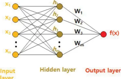
3.2.2.2 Radial Basis Function Network
RBF network is an artificial neural network that uses radial basis function as activation function.
The output of the network is a linear combination of radial basis functions of the inputs and neuron parameters. Radial basis function networks have many uses, including function approximation, time series prediction and classification.
Fig: 7: Output of RBFN in MATLAB.
Radial functions are a special class of function, they could be employed in any sort of model linear or nonlinear and any sort of network single layer or multilayer, but they have been popularly used for single layer network.
Their characteristic feature is that their response decreases or increases monotonically with distance from a central point. The centre, the distance scale
and the precise shape of the radial function are parameters of the model all fixed if it is linear.
A typical radial function is the Gaussian which, in the case of a scalar input is
h(x) = exp(െ (? ? ?)??? )
Its parameters are its centre c and its radius r. A Gaussian RBF monotonically decreases with distance from the centre.
A multi-quadric RBF is as follows
h(x) = ? ??? (? ? ?)??
A multi-quadric RBF monotonically increases with distance from the centre.
Gaussian RBFs are local, give a significant response only in a neighbourhood near the centre and are more commonly used than multi-quadric type RBFs which have a global response.
Fig. 8: Typical Radial Basis Function Network.
In [14], weather information is classified into three classes and corresponding radial basis function neural network providing wind power prediction is activated. Gaussian basis function is used at the hidden layer and centres are estimated by orthogonal least square algorithm, particle swarm optimization algorithm used to determine widths. It has been showed that result obtained from this method is superior as compared to multilayer perceptron.
RBF networks responds faster and give better approximation of desired output [15]. It employs linear learning rule that prevents the network to get struck up in local minima.
x keeping the mathematics simple it is just linear algebra
x the computations relatively cheap there is
no optimization by general purpose gradient descent algorithms
Conclusion
Wind power forecasting is critical to power system operation. However, wind power forecasting errors are unavoidable to some extent due to the nonlinear and stochastic nature of the weather system. This paper presents a comprehensive overview on the wind turbine power curve modeling techniques and mathematical models for wind power forecasting their advantages and disadvantages. These models assist the customers in making the appropriate choice of wind turbines, aid in wind energy assessment and prediction, and revolutionize wind turbine performance monitoring, troubleshooting and predictive control. The various parametric and non-parametric modelling techniques that have been employed for wind turbine power curve
modelling have been presented in detail.
Traditional neural network based forecasting models cannot provide satisfactory performances with respect to both accuracy and computing time needed. Thus, extreme learning machine applied for probabilistic interval forecasting of wind power. Comprehensive experiments using practical wind farm data of National Renewable Energy Laboratory of different season have been done in MATLAB2013a on Processor: Intel(R) Core(TM) i5-3210M CPU @ 2.50GHz, 2501 MHz, 2 Core(s), 4 Logical Processor(s).
References
[1] Vinay Thapar, Gayatri Agnihotri, Vinod Krishna Sethi, “Critical analysis of methods for mathematical modeling of wind turbines”, 10 March 2011.
[2] M. Lydia , S.SureshKumar , .Immanuel Selvakumar , G.Edwin PremKumar , “A comprehensive review on wind turbine power curve modeling techniques”, 21 October 2013.
[3] Shahab Shokrzadeh, Student Member, IEEE, Mohammad Jafari Jozani, and Eric Bibeau, ”Wind Turbine Power Curve Modeling Using Advanced Parametric and Nonparametric Methods”, IEEE TRANSACTIONS ON
SUSTAINABLE ENERGY, VOL. 5, NO. 4, OCTOBER 2014
[4] Guang-Bin Huang, Qin-Yu Zhu, Chee-Kheong Siew, “Extreme learning machine: Theory and applications”, 3 December 2005.
[5] Principe, J.C.; Dept. of Electrical & Computer Eng., Univ. of Florida, Gainesville, FL, USA; Badong Chen” Universal Approximation with Convex Optimization: Gimmick or
Reality?” IEEE Computational intelligence magazine may
2015.
[6] Shuhui Li, Donald C. Wunsch, Edgar O’Hair Michael G. Giesselmann, “Comparative Analysis of Regression and Artificial Neural Network Models for Wind Turbine Power Curve Estimation”, November 2001.
[7] Erik Cambria, Guang-Bin Huang, ”Extreme Learning Machines”, IEEE Computational intelligence December 2013.
[8] Shuhui Li, Member, IEEE, Donald C. Wunsch, Senior Member, IEEE, Edgar A. O’Hair, and Michael G. Giesselmann, Senior Member, IEEE, “Using Neural Networks to Estimate Wind Turbine Power Generation”,IEEE TRANSACTIONS ON ENERGY CONVERSION, VOL. 16, NO. 3, SEPTEMBER 2001.
[9] Can Wan, Zhao Xu, Pierre Pinson, Zhao Yang Dong, Kit Po Wong,” Probabilistic Forecasting of Wind Power Generation Using Extreme Learning Machine”, IEEE
TRANSACTIONS ON POWER SYSTEMS 3, May2014.
[10] Book: WEIFENG LIU, “Adaptive Filtering In Reproducing Kernel Hilbert Spaces”, 2008.
[11] Can Wan, student member; IEEE, Zhao Xu, Senior Member; IEEE, Pierre Pinson, Senior Member ; IEEE, Zhao Yang Dong, Senior Member; IEEE, and Kit Po Wong, Fellow; IEEE,” Probabilistic Forecasting of Wind Power Generation Using Extreme Learning Machine”, IEEE TRANSACTIONS
ON POWER SYSTEMS, VOL. 29, NO. 3, MAY 2014.
[12] W. Frost and C. Aspliden, “Characterics of the wind in Wind Turbine Technology”, D. A. Spera, Ed: AMSE Press, 1995, ch. 8, pp. 371–445.
[13] S. S. Haykin, “Neural Networks: A Comprehensive Foundation”: Macmillan, 1994, p. 160.
[14] George Sideratos and Nikos D. Hatziargyriou, Fellow, IEEE, “Probabilistic Wind Power Forecasting Using Radial Basis Function Neural Networks”, IEEE TRANSACTIONS ON POWER SYSTEMS, VOL. 27, NO. 4, NOVEMBER 2012