University of Windsor University of Windsor
Scholarship at UWindsor
Scholarship at UWindsor
Electronic Theses and Dissertations Theses, Dissertations, and Major Papers
10-19-2015
USING MACHINE LEARNING TECHNIQUES FOR FINDING
USING MACHINE LEARNING TECHNIQUES FOR FINDING
MEANINGFUL TRANSCRIPTS IN PROSTATE CANCER
MEANINGFUL TRANSCRIPTS IN PROSTATE CANCER
PROGRESSION
PROGRESSION
Siva Charan Reddy Singi Reddy
University of Windsor
Follow this and additional works at: https://scholar.uwindsor.ca/etd
Recommended Citation Recommended Citation
Singi Reddy, Siva Charan Reddy, "USING MACHINE LEARNING TECHNIQUES FOR FINDING MEANINGFUL TRANSCRIPTS IN PROSTATE CANCER PROGRESSION" (2015). Electronic Theses and Dissertations. 5433.
https://scholar.uwindsor.ca/etd/5433
This online database contains the full-text of PhD dissertations and Masters’ theses of University of Windsor students from 1954 forward. These documents are made available for personal study and research purposes only, in accordance with the Canadian Copyright Act and the Creative Commons license—CC BY-NC-ND (Attribution, Non-Commercial, No Derivative Works). Under this license, works must always be attributed to the copyright holder (original author), cannot be used for any commercial purposes, and may not be altered. Any other use would require the permission of the copyright holder. Students may inquire about withdrawing their dissertation and/or thesis from this database. For additional inquiries, please contact the repository administrator via email
USING MACHINE LEARNING TECHNIQUES FOR FINDING
MEANINGFUL TRANSCRIPTS IN PROSTATE CANCER
PROGRESSION
by
Siva Charan Reddy Singi Reddy
A Thesis
Submitted to the Faculty of Graduate Studies through School of Computer Science in Partial Fulfillment of the Requirements for the Degree of Master of Computer Science at the
University of Windsor
Windsor, Ontario, Canada 2015
c
USING MACHINE LEARNING TECHNIQUES FOR FINDING
MEANINGFUL TRANSCRIPTS IN PROSTATE CANCER
PROGRESSION
by
Siva Charan Reddy Singi Reddy
APPROVED BY:
L. Porter
Department of Biological Sciences
A. Ngom
School of Computer Science
L. Rueda, Advisor School of Computer Science
Author’s Declaration of Originality
I. Declaration of Previous Publication
This thesis includes one original paper that has been previously published/submitted for
publication in peer reviewed journals, as follows:
Thesis Chapter Publication title/full citation Publication status Chapters 5,6 and appendix Siva Singireddy et al. ”Identifying Differentially Expressed
Transcripts Associated with Prostate Cancer Progression using RNA-Seq and Machine Learning Techniques.” Com-putational Intelligence in Bioinformatics and Computa-tional Biology (CIBCB), 2015 IEEE 12th InternaComputa-tional Conference on. IEEE, 2015.
in proceedings
I certify that I have obtained a written permission from the copyright owner(s) to include
the above published material(s) in my thesis. I certify that the above material describes work
completed during my registration as graduate student at the University of Windsor.
I declare that, to the best of my knowledge, my thesis does not infringe upon anyones
copyright nor violate any proprietary rights and that any ideas, techniques, quotations, or
any other material from the work of other people included in my thesis, published or
oth-erwise, are fully acknowledged in accordance with the standard referencing practices.
Fur-thermore, to the extent that I have included copyrighted material that surpasses the bounds
of fair dealing within the meaning of the Canada Copyright Act, I certify that I have
iv
tained a written permission from the copyright owner(s) to include such material(s) in my
thesis. I declare that this is a true copy of my thesis, including any final revisions, as
ap-proved by my thesis committee and the Graduate Studies office, and that this thesis has not
Abstract
Prostate Cancer is one of the most common types of cancer among Canadian men. Next
generation sequencing that uses RNA-Seq can be valuable in studying cancer, since it
pro-vides large amounts of data as a source for information about biomarkers. For these
rea-sons, we have chosen RNA-Seq data for prostate cancer progression in our study. In this
research, we propose a new method for finding transcripts that can be used as genomic
fea-tures. In this regard, we have gathered a very large amount of transcripts. There are a large
number of transcripts that are not quite relevant, and we filter them by applying a feature
selection algorithm. The results are then processed through a machine learning technique
for classification such as the support vector machine which is used to classify different
stages of prostate cancer. Finally, we have identified potential transcripts associated with
prostate cancer progression. Ideally, these transcripts can be used for improving diagnosis,
treatment, and drug development.
Dedication
With an overflowing heart of thanksgiving, I wish to dedicate this thesis to my God Gifted
Parents Mr. Raja Reddy and Mrs. Shamala. I am also indebted to my loving brother Raja
Shekar Reddy, who took me under his wing in the early years of my education.
Acknowledgements
I would like to start by saying thank you to my supervisor Dr. Luis Rueda, the most
im-portant person and guidance for my research project. I love the unfailing energy,
profes-sionalism, and generosity that you carry in your DNA. The author is profoundly grateful to
Dr. Lisa Porter, Dr. Alioune Ngom, Dr. Dora Cavallo-Medved, and Dr. Iman Rezaeian.
Thank you for your unending and uncompromising support which has enabled me to finish
this thesis. Special thanks to my best friend Abedalrhman Alkhateeb for helping me
com-plete this project. It is a privilege to learn and work with you. Suchet Krishna, Nishanth
Singarapu, Amarender Reddy, Vamshi Reddy, Lal Bahadur Sastry, and Abdul Ameer,
ev-eryone needs friends like you who will extend love, time, and sacrifice in hard times. I am
in debt to you for the rest of my life, thank you all for helping me in my dark times and
encouraging to achieve my ambitions. Many thanks to all of you!
Contents
Author’s Declaration of Originality iii
Abstract v
Dedication vi
Acknowledgements vii
List of Figures ix
List of Tables x
1 Introduction 1
1.1 Prostate Cancer Progression . . . 3
1.2 RNA-Seq . . . 4
1.3 Thesis Motivation . . . 5
1.4 Main Problem . . . 6
1.5 Contributions . . . 6
1.6 Thesis Organization . . . 7
2 Literature Review 8 2.1 Using Genes as Biomarkers . . . 8
CONTENTS ix
2.2 Using Splice Junctions and Transcripts as Biomarkers . . . 10
2.3 Using Methylation Regions as Biomarkers . . . 11
2.4 Conclusion . . . 11
3 Transcriptomics Studies Using RNA-Seq 13 3.1 RNA-Seq Technology . . . 14
3.2 Challenges in RNA-Seq Studies . . . 15
3.3 Sequencing Technologies . . . 16
3.4 Read Alignment . . . 17
3.4.1 UnSpliced Aligners . . . 17
3.4.2 Spliced Aligners . . . 18
3.5 Transcriptome Assembly . . . 19
3.6 Web-Based RNA-Seq tool . . . 20
3.7 Conclusion . . . 21
4 Machine Learning 22 4.1 Classification . . . 22
4.1.1 Support Vector Machine . . . 23
4.1.2 Decision Tree . . . 25
4.1.3 Random Forest . . . 26
4.1.4 Na¨ıve Bayes . . . 27
4.1.5 Multi-class Classification . . . 27
4.2 Feature Selection . . . 28
4.2.1 Chi-squared . . . 29
CONTENTS x
4.3 k-Fold Cross-Validation . . . 30
4.4 Performance Measures . . . 31
4.5 Conclusion . . . 34
5 Methods 35 5.1 Datasets . . . 35
5.2 Data Preprocessing . . . 37
5.3 Classification and Feature Selection . . . 39
5.3.1 Multi-class Problem . . . 41
5.3.2 Feature Selection . . . 41
5.3.3 Classification . . . 42
5.3.4 Performance Evaluation . . . 43
5.4 Biological Significance . . . 43
5.5 Comparison with other methods . . . 44
5.6 Conclusion . . . 45
6 Results and Discussion 46 6.1 Matched Normal Versus Malignant Classification . . . 46
6.1.1 Performance Measures . . . 46
6.1.2 Biological Significance . . . 49
6.2 Prostate Cancer Progression . . . 51
6.2.1 Performance Measures . . . 51
6.2.2 Biological Significance . . . 55
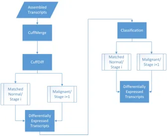
6.3 Comparison with CuffDiff . . . 57
CONTENTS xi
7 Conclusions and Future Work 62
7.1 Contributions . . . 63
7.2 Future Work . . . 63
Appendix A Documentation to run tools 65 A.1 SRA Conversion . . . 65
A.2 Mapping to Reference Genome using Tophat2 . . . 65
A.3 Transcriptome Assembly using Cufflinks . . . 66
A.4 Differential Expression using CuffDiff . . . 66
Appendix B Supplementary Results 67
Appendix C Copyrights Permission 73
Bibliography 74
List of Figures
1.1 Alternative splicing of the gene: DNA translates to RNA; RNA undergoes
splicing and forms mature mRNA; mRNA further translates to a protein. . 2
3.1 Work-flow of an RNA-Seq technology experiment. . . 15
4.1 SVM for linearly separable data. . . 24
4.2 Random forest example. . . 27
4.3 Illustration of thek-Fold cross-validation process. . . 31
4.4 Performance measures used to evaluate the efficiency of a classifier. . . 33
4.5 Receiver operating characteristic. . . 34
5.1 Preprocessing phase of our method: Tophat2 aligns the reads to the ref-erence genome, and Cufflinks assembles the transcriptome and estimates transcript abundance. . . 38
5.2 A sample input file for the classification algorithm. This file is the output of the preprocessing phase. . . 39
5.3 Pipeline of our method for matched normal versus malignant and prostate cancer progression classifications. . . 40
5.4 Workflow for the model we use for comparison. . . 45
LIST OF FIGURES xiii
6.1 Accuracy of classifiers for matched normal versus malignant classification
using mRMR feature selection. . . 48
6.2 AUC of classifiers for matched normal versus malignant classification using
mRMR feature selection. . . 48
6.3 Accuracy of SVM with linear kernel for matched normal versus malignant
classification using chi-squared feature selection. . . 50
6.4 AUC of SVM with linear kernel for matched normal versus malignant
clas-sification using chi-squared feature selection. . . 50
6.5 Expression trend of matched normal versus malignant transcripts. . . 52
6.6 Accuracy of classifiers for pair-wise stage classification using mRMR
fea-ture selection. . . 54
6.7 AUC of classifiers for pair-wise stage classification using mRMR feature
selection. . . 54
6.8 Accuracy of SVM with linear kernel for pair-wise stage classification using
Chi-squared feature selection. . . 56
6.9 AUC of SVM with linear kernel for pair-wise stage classification using
Chi-squared feature selection. . . 56
6.10 Expression trend of Long’s data set transcripts. . . 58
6.11 Accuracy of classifiers for CuffDiff selected transcripts on Long’s data set. 60
6.12 Accuracy of classifiers for our method selected transcripts on Long’s data set. 60
6.13 AUC of classifiers for CuffDiff selected transcripts on Long’s data set. . . 61
List of Tables
1.1 Stages in progression of prostate cancer according to the American Cancer
Society [38]. . . 4
4.1 Example of a two-class classification problem that involves two types of
cancer, matched normal and malignant. . . 23
4.2 Example of a two-class classification problem that involves two types of
cancer, matched normal and malignant. . . 29
5.1 Data sets used in our work. . . 36
5.2 Long’s data set samples in different stages of prostate cancer . . . 37
6.1 Matched normal versus malignant differentially expressed transcripts. . . . 52
6.2 Long’s data set differentially expressed transcripts across different stages. . 58
B.1 Biological significance of Long’s data set transcripts across T1c-T2
pair-wise stage. . . 67
B.2 Biological significance of Long’s data set transcripts across T2-T2a
pair-wise stage. . . 68
B.3 Biological significance of Long’s data set transcripts across T2a-T2b
pair-wise stage. . . 69
LIST OF TABLES xv
B.4 Biological significance of Long’s data set transcripts across T2b-T2c
pair-wise stage. . . 69
B.5 Biological significance of Long’s data set transcripts across T2c-T3a
pair-wise stage. . . 70
B.6 Biological significance of Long’s data set transcripts across T3a-T3b
pair-wise stage. . . 70
B.7 Biological significance of Long’s data set transcripts across T2c-T34
pair-wise stage. . . 71
B.8 Biological significance of matched normal versus malignant classification
Chapter 1
Introduction
A cell, the basic unit of life, is capable of independent reproduction [24]. There are two
kinds of cells: eukaryotic and prokaryotic. In eukaryotic organisms, every cell has a
nu-cleus, while the prokaryotic cell is a unicellular microorganism without a nucleus [24]. The
human body has eukaryotic cells, each with a nucleus at its centre and a cell membrane
for protection [24]. The chromosomes are distributed in the nucleus. Every human cell
has 23 pairs of chromosomes, and each chromosome contains many different genes [1].
Deoxyribonucleic acid (DNA) is used to build and maintain the cell and also carries
hered-itary information within the chromosomes. DNA is composed of nucleotides: adenine (A),
guanine (G), cytosine (C), and thymine (T) [46].
Cells undergo several ways to transform DNA into proteins. Generally, there are two
main steps to convert coding regions of DNA into proteins [24]. In the first step, DNA
transcribes to ribonucleic acid (RNA), while in the second step, RNA translates into proteins
(see Figure 1.1) [9; 20; 24]. The outcome of transcription is the precursor messenger RNA
(pre-mRNA), which undergoes RNA splicing or processing, a process in which exons are
retained and introns are removed [24]. The splicing of pre-mRNA occurs in several different
CHAPTER 1. INTRODUCTION 2
ways. The most common way is that an intron is excluded and an exon is included, which
leads to the formation of a different mRNA strand. This process is known as alternative
splicing [24].
Figure 1.1 illustrates alternative splicing of a gene. DNA contains exons and introns,
also called coding and non-coding regions, respectively. DNA transcribes to RNA, which
further translates to proteins. It can be observed from the figure that exon 1, exon 2, and
exon 4 are retained to form protein 1; exon 1, exon 3, and exon 4 make protein 2. On
the other hand, introns are removed to form the mature mRNA transcript. The study of an
entire group of transcripts or RNA for the diagnosis of precise disease conditions is known
as transcriptomics [45].
Figure 1.1: Alternative splicing of the gene: DNA translates to RNA; RNA undergoes
CHAPTER 1. INTRODUCTION 3
1.1
Prostate Cancer Progression
Prostate cancer is caused by the abnormal and uncontrolled growth of the prostate gland
[40]. According to Statistics Canada, one in five Canadian men will be diagnosed with
prostate cancer during their lifetimes, and one in four will die from prostate cancer [39].
An estimated 196,900 patients are anticipated to be diagnosed with cancer in 2015 [39].
Approximately 50% of these cases will be lung, breast, colorectal, or prostate cancer [39].
Lung cancer accounts for the majority of the cases, followed by colorectal and prostate
cancers [39]. Canadian males are primarily affected by prostate cancer; approximately
24,000 patients are anticipated to be diagnosed with cancer in 2015 [39]. As in other types
of cancer, there is a need to conduct research on prostate cancer. In addition, investigating
prostate cancer at the molecular level can help determine the structure of tumour initiation,
as well as its progression. Prostate cancer is very unlikely to progress; less than one third
of the patients will progress to advanced stages. This kind of investigation aids both the
diagnosis and treatment of the disease at the earliest possible stage.
The American Cancer Society has categorized prostate cancer into four different stages,
each of which is further divided into sub-stages [38; 40]. Table 1.1 provides some
informa-tion about each stage and sub-stage of prostate cancer. Prostate cancer can be discoverable
in the initial stage (T1c) [38]. In the second stage (T2), it spreads to the prostate gland [38].
Stage T2 is divided into three sub-stages (T2a, T2b, and T2c). Cancer grows at a moderate
rate in sub-stages T2a and T2b, whereas growth occurs at a higher rate in stage T2c [38].
At stage T3, the cancer spreads to neighboring tissues. This stage is further divided
into two sub-stages, T3a and T3b [38]. Both sub-stages are essential in prostate cancer
progression, as the cancer spreads to the seminal vesicles in sub-stage T3b [38]. In the
CHAPTER 1. INTRODUCTION 4
invading another organ is known as metastasis [38]. It begins to grow cancer cells in the
new location, thereby damaging the functioning of that organ [38]. Most cancer patients
die when they reach themetastaticstage [38]. Estimating the progression helps in detecting
and diagnosing cancer, and providing a patient with an appropriate treatment.
Table 1.1: Stages in progression of prostate cancer according to the American Cancer So-ciety [38].
Prostate cancer stage Description
T1c The tumour is not detectable via imaging techniques. Can-cer is detected using a needle biopsy performed due to an elevated serum prostate-specific antigen (PSA).
T2 The tumour is palpable, but confined to the prostate.
T2a The tumour is in half, or less than half, of one of the prostate glands two lobes.
T2b The tumour is in more than half of one lobe, but is not in both lobes
T2c The tumour is in both lobes but confined within the prostatic capsule.
T3 The tumour has started spreading out of the prostate tissue. T3a The tumour has spread through the prostatic capsule on one
or both sides, but has not spread to the seminal vesicles. T3b The tumour has invaded one or both of the seminal vesicles.
T4 The tumour has spread to other organs.
1.2
RNA-Seq
RNA-Seq is an emerging technology that uses next generation sequencing (NGS)
tech-niques. It helps biologists and clinicians understand the complexity of diseases at the
molec-ular level [11; 45]. It also provides precise information for analysis of alternative
CHAPTER 1. INTRODUCTION 5
RNA-Seq and NGS have made sequencing costs drop drastically, which has led researchers
to create many RNA-Seq data sets on prostate cancer [45]. We chose RNA-Seq data sets in
our studies for all these reasons, as discussed in more detail in Chapter 3.
1.3
Thesis Motivation
Various studies have found that aberrant splicing of the pre-mRNA yields different kinds of
cancers [49]. The discovery of biomarkers is the central step in diagnosis and handling of
any kind of disease, especially for cancer. Mayer et al. observed that a differential splice
variant, the RON isoform, was upregulated in ovarian cancer [26]. Ren et al. used next
generation sequencing technology and discovered that long non-coding RNAs, gene fusions
and aberrant splicing influence cell growth [33]. Long et al. worked on 106 malignant
samples using RNA-Seq data and extracted 24 genes, of which five genes (BTG2, IGFBP3,
SIRT1, MXI1, and FDPS) correlate with prostate cancer [25].
In recent years, researchers have been working to find biomarkers for different types
of cancer. They have focused mainly on the genetic level and have found differentially
expressed genes. Some researchers have also studied prostate cancer and its progression.
However, investigating the transcriptome activity of a cell or organism is more interesting
than studying it at the gene level, due to the precise information the activity provides on the
disease condition. We examined these kinds of patterns involved in prostate cancer and its
CHAPTER 1. INTRODUCTION 6
1.4
Main Problem
Researchers face the challenging issue of finding biomarkers for prostate cancer; it is
dif-ficult to find them with current approaches [25]. Previous researchers focus on matched
normal versus malignant using genes as biomarkers to find differentially expressed genes
associated with prostate cancer. We are given data sets of RNA-Seq reads that belong to
different samples each associated with particular stage; these samples come from patients
or cell lines. We aim to identify differentially expressed transcripts that are associated with
different stages of prostate cancer. Ideally, these transcripts can be used for improving
diagnosis, treatment and drug development.
To deal with this problem, we applied powerful feature selection and classification
algo-rithms to find discriminative transcripts that are related to prostate cancer and its different
stages.
1.5
Contributions
In this work, we introduce a novel model that integrates emerging RNA-Seq technology
with machine learning approaches to find the vital discriminative transcripts for the different
stages of prostate cancer.
The main contributions are:
• Developing an integrative model that uses feature selection to choose a subgroup
of transcripts and classification techniques to find the most relevant transcripts for
different stages of prostate cancer.
CHAPTER 1. INTRODUCTION 7
1.6
Thesis Organization
This thesis consists of seven chapters, starting with an introduction, which provides an
overview of the main topics. A literature review is presented in Chapter 2. An overview
of RNA-Seq data, workflow, and analysis comprise Chapter 3. In Chapter 4, machine
learning techniques for feature selection and classification are discussed. The methods and
results are discussed in Chapters 5 and 6, respectively. Finally, Chapter 7 presents the thesis
Chapter 2
Literature Review
In this chapter, we review the literature that identifies the problems that researchers are
currently facing in finding biomarkers for prediction of prostate cancer. This chapter is
organized based on the biomarkers used by different scientists. Most of them have used
genes, whereas Tavakoli et al. used junctions, as biomarkers to study prostate cancer. Also,
Kim et al. studied methylation patterns to investigate prostate cancer.
2.1
Using Genes as Biomarkers
Recently, researchers have found it difficult to predict the progression of prostate cancer.
Long et al. worked with genes as biomarkers to estimate the disease development [25]. The
authors gathered tissue cores from 106 prostate cancer patients and extracted RNA-Seq data
[25]. Initially, the RNA was prepared using a formalin-fixed paraffin-embedded approach
and sent for sequencing, which employed the Illumina HiSeq technology to perform 50
base pairs paired-end sequencing [25]. The data set can be retrieved via GEO accession
number GSE54460 [25].
CHAPTER 2. LITERATURE REVIEW 9
Long et al. started their work by following part of the tuxedo suite approach, which
utilizes Tophat2 to align the reads from the patients to the reference human genome and
uses Cufflinks for transcriptome assembly [25]. They used the DESeq tool to find
differ-entially expressed genes [25]. Subsequently, a set of 24 genes were obtained; 16 were
previously associated with prostate cancer, and among them, five genes (BTG2, IGFBP3,
SIRT1, MXI1, and FDPS) are typically associated with prostate cancer [25].
Zhai et al. also worked on RNA-Seq data to find differentially expressed genes that
are related to prostate cancer [47]. They found protein-coding genes and lincRNAs that
are differentially expressed between matched normal and malignant patients [47]. Zhai et
al. experimented on 10 matched prostate samples, which were taken from the European
Nucleotide Archive with accession number SRP002628 [47]. They performed an analysis
that is similar to that of Long et al., except that hierarchical clustering was used for finding
differentially expressed genes [47].
Zhai et al. claims that 10 genes and a lincRNA were differentially expressed [47]. The
authors claim that the lincRNA that is present in the Cullin-associated and
neddulation-dissociated 1 (CAND1) gene expressed high and low between malignant and matched
nor-mal samples, respectively [47].
Ren et al. studied prostate cancer in the Chinese population and revealed that long
non-coding RNAs influence the prognosis [33]. The authors stated that the non-destructive
nature of the prostate cell has no effect [33]. On the other hand, rapidly-advancing cell
growth will lead to metastasis, resulting in the death of the patient [33].
The authors generated RNA-Seq data on the 14 matched prostate samples [33]. The
RNA was gathered from samples, and oligo(DT) primers were used to separate poly(A)
CHAPTER 2. LITERATURE REVIEW 10
and Long’s data sets (discussed in Chapter 5). Ren’s data set used random hexamer primers,
while the other data sets used oligo (DT) primers. The selection of primers is very
impor-tant, since data set extraction depends on the primer used [37]. The two primers have their
own advantages and disadvantages. The choice of primers depends on the mRNA extracted
[37]. If the mRNA contains polyA at the end, usually oligo (DT) is preferable, while if
the mRNA is too long, it is difficult to cover the whole mRNA strand [37; 8]. In this case,
random primers are the best choice, since they are able to extract small pieces of mRNA
[8]. Afterwards, they were divided into fragments, and Illumina HiSeq 2000 was employed
to sequence the reads [33]. Ren et al. aligned these reads by applying the SOAP2 aligner,
and then performed supervised clustering to obtain differentially expressed genes and
non-coding RNAs [33].
Ren et al. studied 183 genes that surprisingly mutated to prostate cancer and three
gene fusions [33]. They found two new gene fusions, CTAGE5-KHDRBS3 and
USP9Y-TTTY15, which are highly linked to prostate cancer, and another gene fusion,
TMPRSS2-ERG, which is quite common in prostate cancer [33].
2.2
Using Splice Junctions and Transcripts as Biomarkers
Tavokoli et al. worked on the problem of finding biomarkers for prostate cancer. They
proposed splice junctions as biomarkers [41]. The authors started their experiment with
Kannan’s data set [5], which has 10 matched samples [41]. The RNA-Seq data was
gener-ated using the Illumina Genome Analyzer II platform [41].
Tavokoli et al. aligned the data set to the reference genome (GRCh37) with the
PAS-Sion tool [41], which outputs splice junctions with cut-off score. They filtered the splice
CHAPTER 2. LITERATURE REVIEW 11
a new scoring scheme was proposed for each junction; afterwards, they applied machine
learning algorithms to these junctions [41]. Finally, when a support vector machine was
used along the junctions, they achieved 100% classification accuracy [41]. They found 10
splice junctions that are highly correlated with prostate cancer [41].
2.3
Using Methylation Regions as Biomarkers
Kim et al. worked on differentially expressed methylated regions that are linked to prostate
cancer [15]. The authors produced a data set with four matched normal and seven malignant
samples by MethylPlex next generation sequencing technology [15].
The RNA-Seq library was prepared with LNCap and PrEC cells for malignant and
matched normal samples, respectively. Kim et al. employed hidden Markov model (HMM)
analysis on the data generated [15]. The reads were produced from enhanced portions that
include all the genes and accession number [15]. To determine the expression level of the
genes, they mapped the reads to the reference genome using the ELAND tool [15].
Kim et al. performed a gene set enrichment analysis (GSEA) to examine the genes
that are differentially-methylated regions [15]. GSEA validates and reports differentially
expressed genes, provided that two conditions are applied. Lastly, they found 2,481
methy-lated regions that are expressed differentially, and WFDC2 was found to be a novel
tumor-methylated region associated with prostate cancer [15].
2.4
Conclusion
The literature review suggests that researchers have recently depended on RNA-Seq data
can-CHAPTER 2. LITERATURE REVIEW 12
cer. Therefore, we have followed a similar tuxedo suite approach in this work. Previous
researchers focus on matched normal versus malignant, while we focus on progression of
prostate cancer. Other works mostly focus on genes as biomarkers and depend on statistical
tests to find differentially expressed genes. However, we focus on transcripts as biomarkers
Chapter 3
Transcriptomics Studies Using RNA-Seq
Analyzing a transcriptome involves determining splice junctions, mRNA, non-coding RNAs,
and post transcriptional alterations of transcripts present in a cell for some specific
experi-mental conditions. The study of transcriptomes is called transcriptomics [45].
There are several methodologies available to study transcriptomes [45]. Each
technol-ogy has its own benefits and drawbacks. Hybridized models, such as microarrays, are
ap-plied to analyze gene expression [45]. They provide reliable output and are cost-effective.
On the other hand, they have disadvantages, such as weak stability of the signals and low
dynamic range of nucleotides [45]. Sanger sequencing was developed to overcome these
limitations of microarrays [45]. Sanger sequencing resulted in an extremely expensive and
very low throughput method, which created a need to develop new approaches [45].
Tag-based approaches create high-end products [45]. However, they generate short reads that
cannot be accurately mapped to the genome. RNA-Seq technology was then developed as
a high-throughput methodology to quantify transcripts [45].
CHAPTER 3. TRANSCRIPTOMICS STUDIES USING RNA-SEQ 14
3.1
RNA-Seq Technology
Wang et al. proposed RNA-Seq, an emerging technology that utilizes next generation
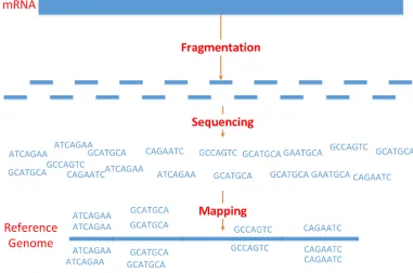
se-quencing techniques to investigate RNAs [45]. Figure 3.1 shows the workflow of an
RNA-Seq technology experiment. Initially, a library is constructed by extracting the RNA from
the underlying samples. Then, the RNA molecules are reverse transcribed to the
corre-sponding complementary DNA (cDNA) fragments. These fragments are defragmented
using RNA or cDNA fragmentation by adding adapters to both ends. Subsequently, the
resulting fragments are amplified in order to obtain the actual short reads; these reads are
then mapped to the reference genome [45].
Small RNA fragments can be sequenced directly. In contrast, mRNA fragments are
usually very large, and hence they are split into shorter fragments before sequencing [6; 45].
To reverse transcribe the RNA, a primer such as an oligo (DT) is attached to the fragments
and converted to cDNA [6]. Adapters are attached to the 5’ and 3’ ends of cDNA. Next, the
fragments are amplified by a polymerase chain reaction (PCR) procedure [6].
RNA-Seq provides short reads, which can produce highly-informative evidence about
the transcripts, and has a particularly superior dynamic range compared to previous
ap-proaches, producing more than 9,000-fold range sequences [45]. RNA-Seq has enhanced
sequence coverage, and has an amazing resolution at a single nucleotide. As such,
RNA-Seq is utilized to discover alternatively spliced RNA, novel isoforms, gene fusions, spliced
CHAPTER 3. TRANSCRIPTOMICS STUDIES USING RNA-SEQ 15
Figure 3.1: Work-flow of an RNA-Seq technology experiment.
3.2
Challenges in RNA-Seq Studies
RNA-Seq technology incorporates multiple steps for library preparation, and manipulation
at each step makes complicated for measuring the transcript expression [45]. Initially, the
entire RNA content of a cell is gathered, which then will undergo sequencing. Previous
surveys indicate that the ribosomal RNA content is high and constitutes more than 80% of
the whole RNA [45]. This leads to a decrease in resource usage, along with a reduction in
sequencing coverage [45]. Therefore, ribosomal RNA is removed by applying an enzymatic
degradation or hybridization-based depletion approach [5; 6].
To achieve higher coverage, deeper sequencing should be performed [45]. This
CHAPTER 3. TRANSCRIPTOMICS STUDIES USING RNA-SEQ 16
coverage, a large genome and a more sophisticated transcriptomics technology are required
[6; 45]. Obtaining such a coverage of a transcriptome has been burdensome until now,
because not all the transcripts are recognize [45]d.
Another challenge of RNA-Seq technology is the representation of gene and exon
bound-aries of the genome [45]. Finding introns and exons is the most difficult part of RNA-Seq
analysis [45]. Aligning the short reads to the reference genome becomes unmanageable for
the aligner tools due to the exon-intron boundaries; identifying the start and end of exons
and introns is extremely difficult [45]. Problems resulting from background noise make this
process very challenging [45].
3.3
Sequencing Technologies
There are several next generation sequencing technologies available in the marketplace.
They can be grouped into two types: single molecule-based and ensemble-based [5]. The
reads that are generated from these sequencing technologies are ready for use in
experi-ments.
There are two kinds of sequencing in RNA-Seq technology: single-end and paired-end
sequencing. In single-end sequencing, the cDNA fragments are sequenced from one end
[5]. This sequencing requires very limited DNA and produces high-quality reads [5]. The
drawback of this mode is that detecting novel isoforms is extremely difficult [5]. In
paired-end sequencing, the fragments are sequenced from both paired-ends to extract the corresponding
reads [5]. This type of reads is very useful in finding novel splice variants, due to the
reorganization of insertions and deletions [5]. The disadvantage of paired-end sequencing
CHAPTER 3. TRANSCRIPTOMICS STUDIES USING RNA-SEQ 17
3.4
Read Alignment
The reads generated by RNA-Seq sequencing technology are aligned to the reference genome
to identify splice sites. There are many tools used for this purpose. They fall into two
cate-gories: unspliced and spliced aligners.
3.4.1
UnSpliced Aligners
An unspliced aligner maps continuous reads to the reference genome. There are several
open source unspliced aligner tools. Bowtie2 is the tool most commonly used by
re-searchers [19]. It is part of the tuxedo approach, being this the reason for which it is applied
in our work.
Bowtie2
Langmead et al. proposed Bowtie2, a fast aligner that employs full-text minute (FM)
in-dexing based on the Burrows-Wheeler transform technique [18]. Langmead et al. made
advancements in the computation of aligning the reads in Bowtie2. This tool divides the
alignment process into four steps. First, reads are divided into seeds with certain base pairs,
using FM indexing. These seeds are aligned to the reference genome; seeds that are not
aligned due to the presence of insertions and deletions are marked and ranked [19]. The
lowest base pair seeds achieve the highest rank, and vice versa. The seeds are then mapped
using single instruction multiple data (SIMD) programming until all the seeds are accessed
CHAPTER 3. TRANSCRIPTOMICS STUDIES USING RNA-SEQ 18
3.4.2
Spliced Aligners
A spliced aligner aligns the spanned exons boundaries[14]. There are two types of spliced
aligner tools: reference-based and de novo-based. The reference-based tools work well
with known spliced junctions (i.e., providing the tool with annotated splice junctions) [14].
On the other hand,de novotools align the spliced reads without prior knowledge of splice
variants of the reference genome [14].
A hybrid spliced aligner tool integrates annotation and de novoalignment. Tophat2 is
such an aligner, which can perform splice alignment with (and without) knowledge of splice
variants, to find novel protein isoforms [14]. We have already discussed in Chapter 2 that
tuxedo is the most common approach used by scientists to extract splice variants. Tophat2,
integrated with Bowtie2, is used in this research as part of the tuxedo approach
Tophat2
Kim et al. addressed a common problem: alignment of RNA-Seq data to the reference
genome to find novel spliced events, which helps in the detection of tumours or cancer
[14]. The authors state that other tools fail to perform accurate mapping if there are higher
expression levels or more insertions and deletions in the genes [14]. Kim et al. describe a
three-step approach for mapping. Initially, Tophat2 uses transcriptome mapping when the
annotation is provided; genome mapping is performed, and spliced mapping is done in the
last step [14]. This approach produces splice junctions and reads accepted by the reference
CHAPTER 3. TRANSCRIPTOMICS STUDIES USING RNA-SEQ 19
3.5
Transcriptome Assembly
Transcriptome assembly involves assembling the reads that have the ability to form
poten-tial mRNA or transcripts [43]. The reads that are accepted by aligner tools to the reference
genome are ready for transcriptome assembly [43]. When transcriptome annotations are
provided, it is a reference-based assembly [43]. On the other hand,de novoassembly means
the tool does not use reference annotations [43]. Subsequently, transcripts’ abundance are
calculated in order to be compared within the same samples or with other samples [43].
Differences in the number of reads obtained from each sample or variations in the length of
the transcripts will change their abundance [43]. Therefore, a normalized value is needed
to compare a transcript with another. There are many ways of computing the normalized
value [43]. The usual means of calculating normalized values is fragment per kilo base of
transcripts per million reads (FPKM) [43]. The fragment refers to both ends of the cDNA,
which is considered one fragment. The per kilo base of transcripts normalizes the
num-ber of fragments dividing by the total numnum-ber of transcripts present in the gene [43]. The
calculation per million reads makes the transcripts comparable to different samples [43].
Cufflinks, a reference-based assembler, is used in our research, because we aim to find
transcripts that are present in the genes and are already associated with prostate cancer
pro-gression [43]. Moreover, Cufflinks is also part of the tuxedo approach. There are other
tools for transcriptome assembly and quantification, including iReckon; we briefly discuss
Cufflinks and iReckon in this chapter.
Cufflinks
Cufflinks is a transcriptome assembler that also estimates the abundance of the transcripts.
CHAPTER 3. TRANSCRIPTOMICS STUDIES USING RNA-SEQ 20
the reference genome. It identifies and filters the reads that are incompatible for assembly.
Reads that are compatible must receive at least one splice junction in common and are the
constituents of the graph being constructed [43].
Trapnell et al. implemented Dilworth’s theorem to cover the minimum path and
con-structed transcripts from the accepted reads [43]. Initially, reads are first marked for
com-patibility. The overlap graph is then constructed such that each transcript present in the
reference transcriptome is covered [43]. Transcript abundance is calculated as the FPKM
value [42]. This value is normalized to verify each transcript with another transcript in the
same gene or other samples [42]
iReckon
Mezlini et al. implemented iReckon, a tool for transcriptome assembly and abundance
es-timation for revealing protein isoforms [27]. iReckon is an implementation of the
regular-ized expectation-maximization (EM) algorithm for construction of transcriptome assembly
and estimating abundance. It discovers potentially novel isoforms by integrating the prior
knowledge of unspliced pre-mRNA and intron retention. Initially, potential isoforms are
identified. The accepted reads from the aligner tools are used to construct the splice graph.
These reads are then rearranged to form potential isoforms [27]. For each transcript, a
nor-malized abundance is calculated such that transcripts are comparable with other transcripts.
3.6
Web-Based RNA-Seq tool
There are many open source standalone tools available. Alternatively, recently-developed
web-based RNA-Seq tools are also used. Galaxy is the most commonly-used web-based
CHAPTER 3. TRANSCRIPTOMICS STUDIES USING RNA-SEQ 21
Galaxy
Blankenberg et al. designed and implemented Galaxy, a web-based open source tool for
Seq analysis [4]. Galaxy offers a wide range of tools to perform analysis on
RNA-Seq data; most of the latest tools used for read alignment, and transcriptome assembly are
installed in Galaxy. The web interface allows users to store data sets and run the tools using
a workflow. Users’ data sets and results can be shared with other users in Galaxy. Galaxy
provides good visualization of the results, and provides source code and documentation so
that the software can be deployed in any server. The advantage of the Galaxy suite works
efficiently on small projects. However, Galaxy cannot accommodate large data sets, due to
memory and space limitations [4]. We have used Galaxy to run Cufflinks on our data sets.
3.7
Conclusion
In this chapter, we discussed about RNA-Seq technology and its challenges. We have also
described different tools that are work on RNA-Seq reads. In the next chapter, machine
Chapter 4
Machine Learning
Machine learning is a branch of artificial intelligence that provides various methods and
al-gorithms that are trained on inputs, and a model is extracted from them [44]. Subsequently,
that model is tested on a different set of inputs, and then the algorithm performance is
mea-sured [44]. Classification and feature selection are two applications of machine learning
[44].
4.1
Classification
The objective of classification is to find a discriminant function from the inputs [44]. There
are three kinds of learning for classification purposes: supervised, unsupervised, and
semi-supervised.
In supervised learning, labeled samples are passed to the classification algorithm, which
creates the predictive model. Figure 4.1 represents a two-class supervised classification
problem; patients are in the rows, while transcripts are in the columns. The last column
contains the class labels: malignant and matched normal samples. We are attempting to
CHAPTER 4. MACHINE LEARNING 23
sign a model that can find a discriminating function between cancerous and non-cancerous
samples. In unsupervised learning, only the samples are given, without the class labels.
Semi-supervised learning uses supervised learning class label knowledge as well as an
un-supervised method for grouping similar data.
Table 4.1: Example of a two-class classification problem that involves two types of cancer, matched normal and malignant.
Samples t1 t2 t3 Class
S1 1 0 1 Malignant
S2 0 0 0 Matched normal
S3 0 0 1 Matched normal
Sk 1 1 0 Malignant
In this thesis, we use supervised learning approaches. Each sample has a class label
that indicates whether or not that sample is matched normal or malignant, or at a
particu-lar stages of prostate cancer. The input vectors are the transcripts that are extracted from
the preprocessing stage, which is discussed in Chapter 5. In the literature, transcripts are
referred to as features, variables, or attributes.
There are many algorithms that have been designed to work on classification problems.
In this thesis, we use support vector machine (SVM), random forest (RF), Na¨ıve Bayes, and
decision tree algorithms, as they worked efficiently for our data sets.
4.1.1
Support Vector Machine
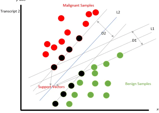
SVM is a classifier that is often used to solve biological problems, among others. It works
efficiently in finding the discriminant function, which is based on the support vectors. There
CHAPTER 4. MACHINE LEARNING 24
4.1 shows an example of linearly separable data. The data is plotted with transcript 1 on the
x-axis and transcript 2 on they-axis. The green-colored points represent matched normal
samples, whereas the red-colored points represent malignant samples. The black-colored
points represent the support vectors.
The goal of an SVM is to find a line that separates the two classes. We can find many
different lines. The SVM tackles this problem by relying on the samples that are the most
difficult to classify, known as support vectors [7]. Initially, the support vectors are
identi-fied, and a line is found, which has the maximum distance from the two classes, this model
is known as hard margin. In Figure 4.1, D2 has the maximum distance as compared to D1;
therefore, line L2 is obtained.
Figure 4.1: SVM for linearly separable data.
CHAPTER 4. MACHINE LEARNING 25
Imagine that, if the data is mapped to a higher dimension, then the line may separate the
data. However, transforming from one dimension to higher dimensions is computationally
expensive. SVM solves this problem by using the kernel trick. If the data becomes linearly
separable, then the line is drawn with the help of the support vectors to separate the classes.
The three most popular kernel methods are: linear, polynomial, and radial basis function.
All of them are used in our research.
Despite using kernel trick sometimes the data is still non-linearly separable [7]. In this
case, SVM uses slack variables on the original data set, which relax the constraints and
penalize the misclassified variable with a cost parameter [7]. The cost parameter is directly
proportional to the slack variable, and acts as a trade-off between the training error rate in
the classification and the maximum width of the margin; this model is termed as soft margin
[7].
4.1.2
Decision Tree
A decision tree is a supervised learning algorithm based on Quinlan’s algorithm used for
classification [30]. The decision tree algorithm builds a tree with a root node and leaves
[30]. The root node is selected based on the information gain value. First, the entropies of
the classes are calculated, and then the entropy of each feature is calculated [30].
Informa-tion gain is the difference between the entropy of the classes and features [30]. The highest
information gain attribute acts as a root node, and each node is constructed based on the
information gain value. The tree is allowed to grow in this manner [30]. Lastly, patterns are
induced by starting from the root, making a decision at each node, following one branch at
each step, ending with a leaf node that corresponds to a certain class. One of the advantages
CHAPTER 4. MACHINE LEARNING 26
4.1.3
Random Forest
Liaw et al. proposed the random forest classifier, which is a model that combines multiple
decision tree predictors [22]. In this classifier, the data set is divided into training and
testing sets. The training set is further divided into two subsets: in the bag and out of the
bag. Two thirds of the training samples are in the bag [22]. They are sampled in such a
way that the number of training samples is equal to the number of samples in the bag. The
sampling is done with replacement, and also known as bootstrapping [22]. The remaining
one-third of the data corresponds to the set that is out of the bag (OOB) [22]. In the bag
samples are input to the decision trees, which learn the classification rules from the given
data used to predict out of bag samples [22].
Figure 4.2 shows how the random forest works, when out of bag samples are given to
them as input. Each decision tree in the random forest will predict the class independently,
based on the OOB data. Each tree votes to which class each sample belongs. The total vote
count is calculated, and the majority-voted class is assigned to that sample. In the figure,
decision tree 1 and decision tree 2 voted for the + class; therefore, class + is assigned to the
sample. The decision tree is grown to the fullest, and there is no need for pruning. Random
forest is really fast and usually achieves very good accuracy for large data sets. For these
CHAPTER 4. MACHINE LEARNING 27
Figure 4.2: Random forest example.
4.1.4
Na¨ıve Bayes
Na¨ıve Bayes is a classification algorithm that uses Bayes’ theorem [34]. It performs
clas-sification based on prior probabilities and likelihoods. Initially, consider a two-class
classi-fication problem [34]. The prior probabilities and likelihoods of both classes are measured
with respect to the new input [34]. Finally, the posterior probabilities for the two classes are
calculated [34]. The class that has the highest posterior probability value is assigned to that
sample [34]. Na¨ıve Bayes classification performance is good when the data is high
dimen-sional; that is the reason for which Na¨ıve Bayes was selected as one of the classification
algorithms [34].
4.1.5
Multi-class Classification
In multi-class classification, there are more than two classes. The classification of stages of
CHAPTER 4. MACHINE LEARNING 28
problem. Two common approaches are one-against-all and one-against-one [22].
In one-against-all, each classifier is trained and tested on one class versus the remaining
classes [22]. If the data set hasrclasses, thenrclassifiers are built in this approach. A class
is assigned to new samples by the classifier that outputs the highest confidence score [22].
All classifiers solve the one-against-all problem in this way [22].
In one-against-one, the classifier is developed for pair-wise classes [22]. Each classifier
classifies a new sample with the class [22]. The class that receives the maximum number of
votes is assigned to that sample [22]. We have adopted a special case of the one-against-one
approach for our classification problem. The model is discussed in Chapter 5.
4.2
Feature Selection
Feature selection is a way of selecting a subset of features from the given data. It is used
to identify and eliminate noisy and redundant features, thereby reducing the dimensionality
of the data. Moreover, feature selection makes classification algorithms operate faster and
more effectively. The goals of feature selection are to reduce the classifier’s complexity and
increase classification accuracy as much as possible.
Consider a pseudo example given in Table 4.2, when all the features (t1,t2, andt3) are
used by the classification algorithm; classification may not work efficiently. However, if
we removet2 and t3, classification might work better as compared to using all features.
Alternatively, if those features are removed then classifier may not necessarily be more
accurate, due to existing interaction among features. Thus, features that have the capability
to discriminate both classes are preserved, while others are removed by feature selection
algorithms. There are two types of feature selection techniques: filter and wrapper methods.
CHAPTER 4. MACHINE LEARNING 29
out irrelevant features. These methods work very fast and ignore any dependencies among
the features. Chi-squared is one of those methods that is used in this research.
Table 4.2: Example of a two-class classification problem that involves two types of cancer, matched normal and malignant.
Samples t1 t2 t3 Class
S1 1 0 1 Malignant
S2 0 0 0 Matched normal
S3 0 0 1 Matched normal
Sk 1 1 0 Malignant
4.2.1
Chi-squared
Chi-squared is a statistical model that calculates a statistical score based on theχ2
distribu-tion. Initially, features are assumed to be independent, andχ2 values are calculated for all
features [23]. The features are then ranked by theirχ2 value in descending order. We have
used chi-squared feature selection in our method, because it operates very quickly and is
less computationally-intensive than other methods in filtering features.
In wrapper methods, all the features are mapped into the feature subset space, and the
classification algorithm is used to select a subset of features. The major advantage of
wrap-per methods is that more informative features are selected, because they consider
interac-tions among the features. On the other hand, the disadvantage is that it is very slow when
there are a large number of features. Using wrapper methods also incurs a higher risk of
CHAPTER 4. MACHINE LEARNING 30
4.2.2
mRMR
Minimum redundancy and maximum relevance (mRMR) is a feature selection method that
depends on mutual information values. The mRMR technique is implemented as a
wrap-per methods, and its main concept is maximum dependency [29]. It selects features in a
two-step process. Initially, mRMR selects the most relevant subset of features that have
maximum relevance for the target class, that is, mutual information [29]. Consider again
the example of Table 4.2 Suppose that we use of featurest1andt2features results in
clas-sification accuracy of 100%. If we then removet2and the classification accuracy is 100%
with only the featuret1, then it is useless to includet2 feature. This approach minimizes
redundancy among the selected subset of features. This is the key benefit of mRMR as
compared to other feature selection algorithms. Since in the main problem addressed in
this thesis we are looking for meaningful transcripts associated with prostate cancer
pro-gression, mRMR is used as a feature selection method. In addition, we have to choose a
classification algorithm, since mRMR is a wrapper method. An SVM with a linear kernel
was used because it yielded good results compared to other classification algorithms, as
shown later in the experimental results.
4.3
k
-Fold Cross-Validation
In this work,k-Fold cross-validation is used for classifier validation. This validation method
works as follows. Initially, the input data are divided intokequal subsets. The classifier is
then trained onk-1 subsets and tested on the remaining part. Figure 4.3 illustrates 10-Fold
cross-validation; we have used 10-Fold cross-validation in our this thesis. The data set is
CHAPTER 4. MACHINE LEARNING 31
part is used for testing the model. This process is iterated 10 times. Finally, the mean of the
desired performance measure is calculated to evaluate the classifier.
Figure 4.3: Illustration of thek-Fold cross-validation process.
4.4
Performance Measures
Performance measures are required to compare the classifiers’ performance on the data sets.
Each classifier reports a confusion matrix, which helps in evaluating the performance of the
classifier. There are many performance measures that can be used to compare classifiers:
accuracy, F-measure, area under the curve (AUC), and the Matthews correlation coefficient
(MCC).
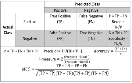
Figure 4.4 represents the formulas for calculating various performance measures.
Con-sider a classification problem in which there are two classes, positive and negative. In the
case of prostate cancer classification, the positives are malignant samples, and the
nega-tives are matched normal samples. In prostate cancer progression classification, the
CHAPTER 4. MACHINE LEARNING 32
For instance, consider the classification of the T3a and T3b classes. The positives are T3b
samples, while the negatives are T3a samples.
Based on Figure 4.4, the actual classes are the labels associated with each original
sample, whereas the predicted classes are the classifier-predicted classes for the samples. A
true positive occurs when a positive sample is predicted as a positive sample, while a false
positive occurs when a negative sample is predicted as a positive sample. Similarly, a false
negative occurs when a positive sample is classified as a negative sample. Lastly, a true
negative occurs when a negative sample is classified as a negative sample.
Generally, accuracy is a good performance metric in the case of balanced data sets.
The higher the accuracy, the better the performance of the classifier is considered (see
Figure 4.4). Precision and recall refer to the positive samples. They focus on how well the
classifier classifies only the positive samples. Recall is also known as sensitivity or true
positive rate. The false positive rate is the difference between 1 and specificity. Precision is
the probability of a sample being positive and actually being predicted as positive. Precision
and recall are inversely proportional to each other. F-measure is the harmonic mean of both
precision and recall. The higher the harmonic mean, the better the classifier is considered.
As shown in the Figure 4.4, the Matthews correlation coefficient (MCC) is considered
to be a balanced performance measure to evaluate a classifier. Referring to the formula
in the figure, MCC deals with all positives and negatives from the confusion matrix. The
MCC value varies from -1 to +1. If the value is close to -1, then the classifier contradicts
the actual and predicted classes. If the value is +1, then the classifier is considered the best
CHAPTER 4. MACHINE LEARNING 33
Figure 4.4: Performance measures used to evaluate the efficiency of a classifier.
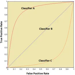
Finally, the receiver operating characteristic (ROC) is a graph that is used to measure
the performance of a classifier. In Figure 4.5, the false-positive rate is plotted on thex-axis,
while the true positive rate is plotted on they-axis for different thresholds. If the classifier
is close to the northwest corner, that classifier is considered the best. If the classifier is
close to the southeast corner, that classifier is considered the worst. From the figure, curves
A, B, and C corresponds to the best, random, and worst classifiers, respectively. However,
a quantitative measure is better suited for comparing classifiers. Thus, the area under the
receiver (AUC) operating characteristic is calculated for this purpose. The classifier with
CHAPTER 4. MACHINE LEARNING 34
Figure 4.5: Receiver operating characteristic.
4.5
Conclusion
In this chapter, we discussed machine learning algorithms used for classification and feature
selection. We have also reviewed cross-validation and performance measures in order to
compare classifiers. In the next chapter, the method that we have developed is examined
Chapter 5
Methods
In this chapter, we discuss the methodology used to work on RNA-Seq data sets in order
to extract transcripts. These transcripts act as potential biomarkers for identifying prostate
cancer and estimating progression stages. Moreover, machine learning techniques, such
as classification and feature selection, were used on these transcripts to find those that are
differentially expressed.
5.1
Datasets
There are many RNA-Seq data sets available for prostate cancer and progression stages
[21]. We selected three data sets that deal with matched normal versus malignant prostate
cancer classification: Kim’s [15], Ren’s [33], and Kannan’s [13]. The data set from Long
et al. [23] was also used, which deals with classification of prostate cancer progression
stages with a large number of samples present in each stage. Ren’s data set used random
hexamer primers, while the other data sets used oligo (DT) primers. All these data sets
are in sequence read archive (SRA) file format and are publicly available from the national
CHAPTER 5. METHODS 36
center for biotechnology information (NCBI) repository [32]. Details about the data sets are
shown in Table 5.1. The second column in the table represents the data set number used by
the NCBI repository [32]. Ren et al. researched prostate cancer in the Chinese population
using 14 matched prostate samples, whereas Kim et al. studied four matched normal and
seven malignant samples. Kannan et al. investigated ten matched prostate samples. Long’s
data set consists of 106 tumour samples.
Table 5.2 depicts the number of samples present in the various stages of prostate cancer
in Long’s data set. The first column in the table identifies the cancer stage, while the
second column specifies the number of patients per stage. The aligner tool that we use
accepts FASTQ/FASTA file formats. All the samples were converted from SRA to FASTQ
file format.
Table 5.1: Data sets used in our work.
Reference Data accession number Number of
samples
Study performed
Long et al. [25] GSE54460 106 malignant Identified differentially expressed genes
Ren et al. [33] ERP000550 14 matched Identified gene fusions
and non-coding RNAs
Kim et al. [15] GSE29155 four matched
normal and
seven malig-nant
Identified methylation patterns
Kannan et al. [13] GSE22260 10 matched Identified alternative
splicing and gene
CHAPTER 5. METHODS 37
Table 5.2: Long’s data set samples in different stages of prostate cancer
Prostate cancer stage Number of samples
T1c 14 T2 10 T2a 23 T2b 11 T2c 30 T3 2 T3a 6 T3b 8 T4 1
5.2
Data Preprocessing
All SRA file format samples were converted to FASTQ files and sent to the preprocessing
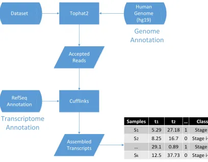
stage. Figure 5.1 shows a diagram for the preprocessing step performed on the data sets in
order to extract the transcripts. Tophat2 is used to align the reads. The inputs to Tophat2
are the FASTQ files from the patients and human genome (hg19) [17]. This tool outputs the
reads that are aligned to the reference genome, which are known as accepted reads.
Cuf-flinks is then used to perform transcriptome assembly. The inputs to this tool are accepted
reads and transcriptome annotation (RefSeq) [31]. Cufflinks outputs transcripts that are
as-sembled for which their abundance are calculated using FPKM values. This preprocessing
step is repeated for each sample.
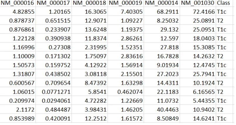
For each data set, we constructed a table with transcripts the corresponding FPKM
values for each sample. Figure 5.2 shows a sample table, which contains the transcripts
and their FPKM values. We already know that each sample belongs to a matched normal
or malignant class, or to a different stage of prostate cancer. This is represented in the last
CHAPTER 5. METHODS 38
Figure 5.1: Preprocessing phase of our method: Tophat2 aligns the reads to the reference
CHAPTER 5. METHODS 39
Figure 5.2: A sample input file for the classification algorithm. This file is the output of the
preprocessing phase.
5.3
Classification and Feature Selection
We have used Weka, a data mining tool that integrates feature selection and classification
algorithms [12]. Weka is an open-source Java tool developed by the University of Waikato
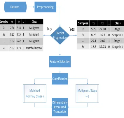
and is widely used for data mining in bioinformatics and other fields. Figure 5.3 shows
the pipeline of our proposed method. The preprocessing step produces a table that contains
transcripts and their FPKM values, as discussed in the previous section. In the figure,
there are two tables. The one on the left is for matched normal versus malignant tumour
classification, and the one on the right is for prostate cancer progression. These two tables
act as inputs to the feature selection algorithm, which will filter out noisy and redundant
transcripts.
CHAPTER 5. METHODS 40
the samples based on the classification rules learned in the training phase. Finally, the
differentially expressed transcripts are obtained.
10-Fold cross-validation is performed on the classifiers to maintain their generalization
capability on the test set. Performance measures are used to evaluate the performance of
the classifiers on different data sets.
Figure 5.3: Pipeline of our method for matched normal versus malignant and prostate
CHAPTER 5. METHODS 41
5.3.1
Multi-class Problem
Since we deal with different stages of prostate cancer, we model the problem as a
multi-class multi-classification problem. We have already discussed the multi-multi-class problem in Chapter
4. For this research, we consider a special case of the one-against-one scheme.
All biological processes are continuous. Consider cancer progression, in which the
can-cer continuously grows at each stage. Moreover, we are interested in finding differentially
expressed transcripts between neighboring stages. In Long’s data set, we have resolved
the multi-class problem by comparing samples between neighboring stages, such as T1c
with T2, and T2 with T2a. Another challenge in Long’s data set is that there are very few
samples in some stages, such as T3 and T4. This may cause a classifier to suffer from the
problem of over-fitting, due to a large number of features. To avoid this, we have merged
T3 samples with the T3a stage into one class calledT3aand T4 samples with the T3b stage
into a single class calledT3b.
We are more concerned about finding differentially expressed transcripts from T2 to T3
stages, because they play a vital role in progression of prostate cancer. In the T3 stage,
the tumour growths rapidly and aggressively to eventually getting closer to the metastasis
stage. Therefore, in addition to considering neighboring stages, we have also added another
class as a result of merging all the samples from stages T3, T3a, T3b, and T4; we call this
class T34.
5.3.2
Feature Selection
Feature selection has been previously discussed in Chapter 4. We have used feature
se-lection because the preprocessing stage extracted 43,497 transcripts per sample. Applying

![Table 1.1: Stages in progression of prostate cancer according to the American Cancer So-ciety [38].](https://thumb-us.123doks.com/thumbv2/123dok_us/1401201.1172782/20.612.117.525.257.495/table-stages-progression-prostate-cancer-according-american-cancer.webp)