Laut, Ingo (2017): Nonreciprocity and nonlinearity: applications in complex plasmas and time series. Dissertation, LMU München: Fakultät für Physik

Nonreciprocity and nonlinearity:

Applications in complex plasmas

and time series

Ingo Joachim Laut

Nonreciprocity and nonlinearity:

Applications in complex plasmas

and time series

Ingo Joachim Laut

Dissertation

an der Fakultät für Physik

der Ludwig-Maximilians-Universität

München

vorgelegt von

Ingo Joachim Laut

aus München

Zweitgutachter: Prof. Dr. Hartmut Zohm

Contents

Zusammenfassung vii

Abstract ix

1 Introduction 1

1.1 Nonlinear time series analysis . . . 1

1.1.1 Phase space representation . . . 1

1.1.2 Fourier representation . . . 3

1.1.3 Measures for nonlinearity . . . 4

1.1.4 Surrogate data . . . 7

1.2 Complex plasmas . . . 9

1.2.1 Basic Properties of Complex Plasmas . . . 10

1.2.2 Nonreciprocity effects in complex plasmas . . . 14

1.2.3 Molecular-dynamics simulations . . . 18

1.2.4 Characterizing complex plasmas . . . 20

1.3 Aims of this thesis . . . 22

2 Synchronization during the mode-coupling instability 25 2.1 Objectives . . . 25

2.2 Methods . . . 26

2.3 Results . . . 28

2.4 Conclusion . . . 30

3 Self-propelled motion of an extra particle 33 3.1 Objectives . . . 33

3.2 Methods . . . 33

3.3 Results . . . 34

3.4 Conclusion . . . 40

4 The role of Fourier phases in nonlinear time series 41 4.1 Objectives . . . 41

4.2 Methods . . . 42

4.3 Results . . . 43

4.4 Conclusion . . . 46

A Enclosed papers 49

Synchronization of particle motion in compressed two-dimensional plasma crystals (Ref. [102]) . . . 50 Anisotropic confinement effects in a two-dimensional plasma crystal (Ref. [113]) 58 Wake-mediated propulsion of an upstream particle in two-dimensional plasma

crystals (Ref. [121]) . . . 70 Time series with tailored nonlinearities (Ref. [126]) . . . 76 Surrogate-assisted network analysis of nonlinear time series (Ref. [127]) . . . 82

Zusammenfassung

Newtons drittes Gesetz von Aktion und Reaktion ist ein Grundpfeiler der klassischen Mechanik. In Nichtgleichgewichtssystemen kann dieses Gesetz durch effektive Wechsel-wirkungen, welche durch einen weiteren Körper vermittelt werden, gebrochen werden. In ähnlicher Weise bereicherte die Entdeckung des deterministischen Chaos das Gebiet der Zeitserienanalyse. Im Rahmen dieser Dissertation werden dynamische Effekte, die auf der nichtreziproken Wechselwirkung in komplexen Plasmen basieren, und der Einfluss der Fourierphasen nichtlinearer Zeitserien untersucht.

In einem komplexen Plasma, welches aus geladenen Mikropartikeln in einem schwach ionisierten Plasma besteht, können strömende Ionen die Rolle dieses weiteren Körpers übernehmen. Der erste untersuchte Effekt ist die Modenkopplungs-Instabilität, bei der bestimmte Schwingungsmoden in einem zweidimensionalen Plasmakristall exponentiell wachsen. In Simulationen wird gezeigt, dass die Instabilibät durch ein anisotropes horizon-tales Potential in einer asymmetrischen Art und Weise ausgelöst werden kann. Dadurch wird die Instabilität in nur zwei oder vier der sechs möglichen Richtungen aktiviert. In sehr guter Übereinstimmung zu früheren Experimenten wird während der asymmetrisch ausgelösten Instabilität eine synchronisierte Teilchenbewegung beobachtet. Es wird ein Ordnungspa-rameter entwickelt, der das richtungsabhängige Synchronisationsmuster quantifiziert. Es werden mögliche Mechanismen diskutiert, die zu einem weiteren Symmetriebruch führen der nicht durch das anisotrope Potential erklärt werden kann.

Ein weiterer Effekt, der auf nichtreziproken Wechselwirkungen basiert, ist der Git-terführungseffekt (englisch channeling). Ein zuätzliches Teilchen, welches nicht Teil des zweidimensionalen Kristallverbunds ist, bewegt sich knapp überhalb des Kristalls mit annähernd konstanter Geschwindigkeit auf einer durch die Kristallstruktur vorgegebenen Bahn. Der Effekt wird in Simulationen reproduziert. Aufgrund der Nichtreziprozität der Wechselwirkungen zieht das zusätzliche Teilchen umliegende Teilchen an, während es selbst eine repulsive Kraft von den sich annähernden Teilchen erfährt. Dies führt zu einem intrinsischen Antrieb des Teilchens. Mit einem einfachen theoretischen Modell für den Antriebsmechanismus kann die Geschwindigkeit des zusätzlichen Teilchens vorhergesagt werden.

Die Tatsache, dass die gesamte nichtlineare Information einer Zeitserie in den Fourier-phasen kodiert ist, wird in einigen Algorithmen zur Surrogaterzeugung genutzt, hat darüber hinaus jedoch keine große Beachtung gefunden. In dieser Arbeit wird gezeigt, dass Korre-lationen in den Fourierphasen Nichtlinearitätsmaße beeinflussen können. Es wird gezeigt,

Abstract

Newton’s third law of action and reaction is one pillar of classical mechanics. In nonequilib-rium systems this fundamental law can be broken when the effective interaction is mediated by a third body, enabling surprising and counterintuitive effects. In a similar manner, the discovery of deterministic chaos in nonlinear systems enriched the field of time series analysis. This thesis covers dynamical effects based on nonreciprocal interactions in complex plasmas and sheds a light on the role of the Fourier phases in nonlinear time series.

In a complex plasma, which consists of charged microparticles immersed in a weakly ionized gas, streaming ions can play the role of the third body in the microparticle interaction. As a first nonreciprocity effect, the asymmetric triggering of the mode-coupling instability, where some wave modes in a two-dimensional plasma crystal grow exponentially with time, is studied in molecular-dynamics simulations. It is shown that an anisotropic confinement in the horizontal plane can trigger the instability in only two or four out of the six directions that are allowed in the hexagonal crystal lattice. In very good agreement with previous experimental observations, the asymmetric triggering of the instability is accompanied by a synchronized motion of the particles. A novel order parameter is developed to quantify the direction-dependent synchronization pattern. Possible mechanisms leading to a more delicate symmetry breaking that cannot be explained by the anisotropic confinement are also discussed.

A second effect based on nonreciprocal particle interactions is the channeling mechanism, where an extra particle that is not part of the two-dimensional crystal lattice floats slightly above the crystal and moves with almost constant velocity through a channel formed by the lattice. The mechanism is reproduced in simulations. It is shown that due to the nonreciprocity of the interactions, the extra particle attracts nearby particles, while it is itself repelled from the approaching particles, leading to a self-propelled motion of the extra particle. A simple theoretical model for the propulsion is provided which predicts the velocity of the extra particle.

The fact that all nonlinearities of a time series reside in the Fourier phases is implicitly used in many schemes for generating surrogates, but has not received much attention beyond that. Here, correlations in the Fourier phases are shown to have an impact on the nonlinear properties of a time series. Spurious phase correlations in amplitude-adjusted surrogates, that should be devoid of nonlinear information, can in turn lead to a nondetection of nonlinearity. Finally, by comparing different nonlinearity measures, the nonlinear prediction error is found to be superior to more recent measures derived from network theory.

Chapter 1

Introduction

1.1

Nonlinear time series analysis

One main goal of nonlinear time series analysis is to determine whether a system has underlying chaotic dynamics [1, 2]. To this end, some measure of nonlinearity, most of which are derived from chaos theory, is calculated for the time series. As the outcome of most tests for nonlinearity yields a numerical value that alone cannot confirm or exclude the presence of nonlinearity, the measure is often also applied to surrogate data which mimic the linear properties of the original data but contain no nonlinearities. If nonlinearity is found in such a statistical test in a time series, purely linear models to describe the underlying physics can be ruled out.

1.1.1

Phase space representation

In his much renowned paper on cellular convection, Lorenz conjectured that low-dimensional, deterministic equations can show chaotic behavior in such a way that “prediction of the sufficiently distant future is impossible by any method, unless the present conditions are known exactly” [3]. The geometric shape of such a strange attractor in phase space cannot be described by an integer dimension, which led to the development of a multitude of dimensionality measures for chaotic systems.

In Fig. 1.1(a)–(d) are shown snapshots of the time evolution of 50 different realizations of trajectories on the attractor of the Lorenz system [3],

dx

dt =σ(y−x),

dy

dt =x(ρ−z)−y,

dz

dt =xy−βz,

(1.1)

where σ= 10, β= 8/3 and ρ= 28. Initially, at t= 0, the trajectories are within a small distance in phase space. First, the strong dependence on the initial conditions leads

x

0 5 10 15₂₀ 3020

y

102030

z

0 10 20 30 40 50

x

0 5 10 15₂₀ 3020

y

102030

z

0 10 20 30 40 50

x

0 5 10 15₂₀ 3020

y

1020 30

z

0 10 20 30 40 50

x

0 5 10 15₂₀ 3020

y

1020 30

z

0 10 20 30 40 50

x

20 30 6040

y

2040

z

4060 80 100120

140160

a

)

t

=12

.

50

b

)

t

=14

.

25

c

)

t

=16

.

50

d

)

t

=30

.

00

e

)

t

=30

.

00

1.1. Nonlinear time series analysis 3

to a spread of the different realizations in a direction tangential to the trajectories, see Fig. 1.1(a, b). The realizations then further spread (c) until they are scattered over the full attractor (d). This “unpredictability” of the dynamics of trajectories that are initially close in phase space is most striking when compared to the dynamics of the system in the linear regime shown in Fig. 1.1(e).

If not all variables of a dynamical system can be observed, it is difficult to fully characterize the system. Often, only one observable is available from a measurement of a system that is expected to depend on more than one parameters. The full dynamics of the system can then be regained by embedding the time series in an appropriate higher-dimensional phase space. Takens addressed the question how the phase space of an attractor could be reconstructed from this time series of observables [4]. He proved that there exists an embedding, i. e., a continuous mapping of the time series to an embedding space that is topologically equivalent to the attractor. The embedding is called delay-time embedding of a time series _{yi_} and reads [5]

yn= (yn−(d−1)τ, yn−(d−2)τ, . . . , yn) (1.2)

where d is the embedding dimensions and τ the delay time.

If the embedding dimension is too small, points may be near to one another only because the attractor is projected onto a lower dimension. With the false neighbor method [6], an appropriate embedding dimension d can be found by analyzing how the fraction of false neighbors decreases with increasing d. For determining an appropriate delay time τ two values can be considered: the first zero-crossing of the autocorrelation function or the first minimum of the mutual information [7].

1.1.2

Fourier representation

An elegant definition of “nonlinearity” can be given with the Fourier representation

F T[_{yn_}] = 1

N X

n

yne2πikn/N =_|ak_|eiφk (1.3)

of a time series _{yn} of length N. All linear information is contained in the Fourier amplitudes _|ak|, while all nonlinear information is contained in the Fourier phases φk. The reasoning is as follows. The linear properties of a time series are those that can be reproduced by an autoregressive (AR) process of the form

yn=µ+X

i

ciyn₋i+n, (1.4)

where µ is a constant, n is uncorrelated noise and the ci are the parameters of the process. The Yule-Walker equations [8, 9] relate the ci of the corresponding AR process to the autocorrelation function

ACF[_{yn_}] =X

n

of the time series. Since the Wiener-Khinchin theorem [10] is a bijective relation between the autocorrelation function and the power spectrum _{|ak_|2_{}given by}

F T[ACF[_{yn}] ] =|ak|2, (1.6)

the linear information of a time series is solely contained in the magnitude of the Fourier coefficients _|ak_|. As a consequence, the nonlinear information is encoded in the Fourier phases. This argument is often used for the generation of so-called surrogate data (see Sec. 1.1.4) that mimic the linear properties of a time series, but have all nonlinearities destroyed.

1.1.3

Measures for nonlinearity

Correlation dimension

Measures for nonlinearity can be divided into two classes, namely static and dynamic measures. Static measures take the data set as a whole into consideration and describe the distribution of the data points in phase space. Dynamical measures, in contrast, also take the time dynamics into account that are encoded in the underlying equations or can be reconstructed from the embedded data if the equations are not known.

The dimension estimates mentioned in Sec. 1.1.1 are static measures. One prime example is the correlation dimension D2. As a first step, one calculates the correlation dimension

C(r) = 1

N(N + 1)

X

n,j

θ(r−rnj) (1.7)

for different values of r. rnj =krn−rjk andθ is the Heaviside function. If the growth of C(r)with radius r obeys a power law, the correlation dimension can be associated with the slope ofC(r)in a double-logarithmic scale:

D2 = lim r→0Nlim→∞

dlogC(r)

dlogr . (1.8)

The attractor of the Lorenz equations shown in Fig. 1.1(a)–(d) has a non-integer correlation dimension of D2 = 2.05±0.01[11].

Nonlinear Prediction Error

The nonlinear prediction error is an example of a dynamical measure for nonlinearity [12, 13]. The idea is that for a deterministic system, points that are close to each other in phase space have a comparable time evolution. By averaging over the future positions of the neighbors of a point yn, an estimateF(yn, T) for the future position is obtained as

F(yn, T) = 1

g X

j∈Ug(n)

1.1. Nonlinear time series analysis 5

20 15 10 5 0 5 10 15 20

x

15 10 5 0 5 10 15 20

x

20 15 10 5 0 5 10 15 20

x

15 10 5 0 5 10 15 20

x

0.0 2.5 5.0 7.5 10.0 12.5 15.0 17.5 20.0En 0.000 0.005 0.010 ν 0.015 0.020 0.025

a)

b)

Figure 1.2: (a) Local nonlinear prediction error_Enfor the Lorenz system. Gray lines connect

points in embedding space that correspond to successive time steps. (b) Degree centrality

κν derived from a recurrence network. Gray lines connect points that are connected in the network. For the visualization of the network, every node ν is located at the point in phase space that it corresponds to.

where Ug(n) is the set of indices of the g nearest neighbors of point yn and T is the lead

time. The local nonlinear prediction error is then the distance from this estimate to the actual future position in phase space y_n+T,

En= q

kyn+T −F(yn, T)k2, (1.10)

and the global nonlinear prediction error is obtained by averaging over all points in phase space _E=p_hE2

nin.

The local nonlinear prediction error _En for the Lorenz system (see Eq. 1.1) is shown

in Fig. 1.2(a). 2000 data steps of thex coordinate with a step size of 0.08 time units are considered. The data are embedded in d= 3 dimensions with a delay time of τ= 0.16. The arrangement of the embedded points resembles the butterfly-shaped structure of the original Lorenz system shown in Fig. 1.1. For g= 4 and a lead time of T= 5,_En is small for

Recurrence network

With the substantial success of complex network theory in various fields of physics [14–17], it has recently also been applied to time series analysis. As there is no “natural” way of how to create a network from a time series, different procedures have been suggested to translate the data into nodes and edges of a network [18–21]. One procedure is therecurrence network

[20, 22, 23] which contains the information which points are sufficiently close to each other in phase space. The adjacency matrix A of the recurrence network [23] reads

Amn() = Θ (_{− k}ym−ynk)−δmn, (1.11)

where the _{yn} are the (embedded) points of the time series in phase space and an

appropriate threshold. The recurrence network as defined by Eq. 1.11 is an unweighted network as Amn can only take two values: it is unity if there is a connection, or edge,

between nodes m and n, and zero otherwise. The Kronecker delta in Eq. 1.11 prevents self-loops such that Ann= 0.

Once the recurrence network is obtained for a time series, it can be analyzed with different network measures. The most prominent measure for any network is the degree centrality kν which counts the number of nodes that are connected to node ν [24],

kν = N_X−1

i=0

Aν,i. (1.12)

Dividing by the maximum possible value yields the connectivityκν. The average connectiv-ity κ is defined as the mean of all nodes κν,

κ= 1

N N_X−1

ν=0 κν =

1

N(N −1)

N−1 X

ν=0

kν. (1.13)

Other measures include the clustering coefficient which is the fraction of neighbors of a nodeν that are themselves connected and the average path length fromν to any other node of the network. In Ref. [20], the bifurcation diagram of the logistic map, a one-dimensional nonlinear system, was analyzed. Different regimes such as period doublings and chaos were identified by dynamical changes of the measures as the control parameter was varied.

Symbolic network

1.1. Nonlinear time series analysis 7

In the symbolic network proposed in Ref. [25], each time step n is associated with a symbol-pair containing the amplitude information α(n) and the ordinal patternπ(n). The former is calculated by binning the time series in the interval [min({yn}),max({yn})] into

Qequal regions. α(n)is then simply the bin number of yn. To compute π(n), one considers the sequence [yn, yn+τ, ..., yn+(L−1)τ] for a given time-delay τ and window length L. The

ordinal pattern π(n) = (β1, β2, ..., βL) contains the indices sorting the sequence such that yn−1+β1 ≤ yn−1+β2 ≤ ...≤ yn−1+βL. The symbol-pair at step n, (α(n), π(n)), is then one

node of the network, and it is connected by a directed link to the symbol-pair (α(n+1),

π(n+ 1)) of the successive time step. In this representation, different time steps may correspond to the same symbol-pairs. Only nodes whose symbol-pairs are present in the time series are part of the network, the actual number of nodes may thus be smaller than the maximal possible value Nmax_=Q·L!.

1.1.4

Surrogate data

Surrogates are ersatz data which have the same linear properties as the original time series, but contain no nonlinearities. They provide a statistical test for a nonlinearity measure M

in a model-independent way. The outcome of measure M of the original time series under study is compared to the outcomes _{Ms_} of the surrogate data. The significance of the deviation of the time series from a set of surrogates is calculated as

S(M) = |M − h{Ms}is|

σ({Ms}) , (1.14)

where _h{Ms_}is and σ({Ms})are the mean and standard deviation of the outcomes of the

measures _{Ms} for the surrogate data.

Surrogate generating algorithms rely on the definition of nonlinearity that was given in Sec. 1.1.2, which states that all nonlinear information of a time series is contained in the Fourier phases. The most popular algorithms thus randomize the Fourier phases in order to remove potential nonlinearities present in the time series while preserving the autocorrelation function. Alternatively, the time series can be shuffled to destroy the nonlinearities, but then also the autocorrelation function is changed and has to be restored in an iterative scheme. Below, different surrogate generating algorithms are presented.

y(t) _|A(k)|eiφ(k) |A(k)|eiφr(k) y s(t)

F T randomize

phases

F T−1

y(t)

e

y(t) _|A(k)|eiφ(k) |A(k)|eiφr(k) y_e

s(t) ys(t)

ROR on Gauss

F T randomize

phases

F T−1

ROR ony(t)

y(t) _y{_si}_(t)

A{i}(k)eiφ{i}(k)

|A0(k)_|eiφ{i}(k)

e

ys{i}(t)

shuffle time series

F T

replace Fourier amplitudes

F T−1

ROR ony(t)

a)

b)

c)

Figure 1.3: Surrogate generating schemes. (a) FT surrogate. (b) AAFT surrogate. (c) IAAFT surrogate. Both the AAFT and IAAFT schemes use a rank-ordered-remapping (ROR) step. FT surrogates do not have a remapping step, but can only be applied to time

1.2. Complex plasmas 9

{ξn}. The reordered_{ξn}thus “follow” the original time series_{yn}while having a Gaussian amplitude distribution.

Amplitude-adjusted Fourier-transformed (AAFT) surrogates can be generated for time series with arbitrary amplitude distribution [26]. As sketched in Fig. 1.3(b), a copy of the original time series is first rank-ordered-remapped to a Gaussian distribution. Then, a FT surrogate of this remapped time series is created. Finally, the surrogate is rank-ordered-remapped to the original time series. The surrogate has the same amplitude distribution as the original time series, but a slightly broader power spectrum due to the final remapping step. As the remapping is done after the phase randomization, new correlations are can be introduced in the Fourier phases. Moreover, in Ref. [27] it was shown that the broader power spectrum may lead to an erroneous detection of nonlinearity in purely linear data.

The iterated amplitude-adjusted Fourier-transformed (IAAFT) surrogates were designed to overcome the shortcoming of AAFT surrogates described in Ref. [27]. The Fourier amplitudes _|A0(k)| of the original time series y(t) are initially saved. Then, as sketched

in Fig. 1.3(c), the scheme starts with a random shuffle ys{0}(t) of y(t). Now, the following

two steps are repeated iteratively. (1) Take the Fourier transform of y{si}(t), replace the

corresponding Fourier amplitudes by _|A0(k)| and transform back. The resulting time series e

y{si}(t) has now exactly the same autocorrelation function as the original time series, but

not the same amplitude distribution. (2) Rank-ordered-remap y_e{si}(t) to y(t) to obtain y{si+1}(t) for the next iteration. The IAAFT scheme stops when the remapping step leads

to no reordering of the time series.

The IAAFT surrogates reproduce both the autocorrelation and the amplitude spectrum of the original time series. However, the randomness of the Fourier phases that is only given at the very beginning of the iteration scheme can no longer be guaranteed. The rank-ordered-remapping step of the AAFT and IAAFT schemes can induce spurious phase correlations in the surrogates. It was shown in Ref. [28] that induced phase correlations in AAFT and IAAFT surrogate data can lead to a nondetection of weak nonlinearities.

1.2

Complex plasmas

a)

b)

c)

Figure 1.4: Complex-plasma experiments. (a) Side view of a large three-dimensional cloud in the PK-3 Plus laboratory onboard the International Space Station [39]. (b) and (c): Top view and side view of a two-dimensional plasma crystal in the Large Chamber in the research group of complex plasmas. Courtesy of John Meyer. For (a) and (c), the approximate positions of the bulk plasma, the plasma sheath and the electrode are shown to the left.

1.2.1

Basic Properties of Complex Plasmas

Most experiments with complex plasmas can be divided into two classes. First, large three-dimensional homogeneous structures can be obtained under microgravity conditions or with thermophoresis [38]. The particles levitate in the quasineutral bulk plasma. Microgravity conditions are met onboard the International Space Station [39] and during parabolic flights [40]. Various crystal geometries, like bcc, fcc and hcp lattices, can be observed. A typical side view is shown in Fig. 1.4(a). In the second class of experiments, in ground-based laboratories, particles levitate in the plasma sheath region above the lower electrode, where there is a force balance between, primarily, the gravitational and electrostatic forces (see Fig. 1.4(b) and (c)). The plasma sheath is the boundary region of positive space charge where an electric field decreases from the electrode to the bulk plasma [41]. In the sheath, the particles form extended structures consisting of 104_–105 _{particles arranged in one or a}

few horizontal layers. In a layer, the particles can form a hexagonal lattice.

The most important elementary processes in complex plasmas are the charging of the particles, the screening of the resulting electrostatic potential through the electrons and ions of the plasma, and the momentum transfer from flowing ions to the particles [35, 36]. The processes have a large impact on the external forces acting on the particles, and on the mutual particle interactions that will also be discussed in the following.

Particle charging

1.2. Complex plasmas 11

due to electrostatic repulsion and the electron and ion fluxes are balanced. A well-known approach to calculate the fluxes is the orbital motion limited (OML) approximation, where the cross section determining the fluxes are derived from the conservation laws of energy and angular momentum. A single particle in a collisionless isotropic plasma is assumed. In this theory, the normalized surface potential z=φse/kBTe only depends on the electron-to-ion temperature ratioτ=Te/Ti and the electron-to-ion mass ratio (determined by the gas used). For typical parameters τ ' 10–100 one obtains z ' 2–4 [35]. For small particles with a radius ap λ, where λ is the Debye screening length, the charge is given by Q=apφs, and thus increases linearly with particle radius ap. For typical values, ap = 1 µm and

kBTe= 1 eV, the charge is Q=−(1–3)×103_{e [35]. The effect of plasma flow anisotropy}

and ion-neutral collisions on the charging process can be taken into account using more complicated approaches, such as particle-in-cell simulations [42, 43].

Screening

The electrostatic potential φ(r) around a spherical charged particle of radius ap in an isotropic and collisionless plasma obeys the Poisson equation

4φ=−4πe(ni−ne) (1.15)

with the boundary conditionsφ(∞) = 0andφ(ap) =φs[35]. niandneare the ion and electron densities which also depend on the potentialφ and distancer[44, 45]. The surface potential

φs at the particle radius ap is connected to the particle charge Q through dφ_dr

r=ap=−Q/a 2 p.

An exact solution for Eq. 1.15 can be obtained numerically, or various approximations can be made to obtain analytical solutions. Assuming a Boltzmann distribution for ions and electrons

ne,i =n0e±eφ/kBTe,i, (1.16)

where n0 is the unperturbed plasma density, and further assuming |eφs/kBTe,i| 1 and ap λ, one obtains the Debye-Hückel (Yukawa) potential

φ(r) = Q

r exp

−_λr. (1.17)

The linearized Debye length λ=λeλi/ p

λ2

e+λ2i is expressed as function of the electronic

and ionic Debye lengthsλe,i=pkBTe,i/(4πn0e2). The absorption of plasma particles on the

particle surface has a great influence on the electrostatic potential. While this effect is rather weak for electrons, the ion flux on the particle makes the ion distribution non-Boltzmann. In the absence of ion-neutral collisions, the ion flux leads to a power-law dependenceφ(r)∝r−2

in the far-field of the potential [35, 46]. In the other limit of a strongly collisional plasma, the far-field instead has a Coulomb-like dependence φ(r) _∝r−1 _{[47, 48]. As the far-field}

limit can often be neglected, the bare Yukawa potential of Eq. 1.17 is often used in isotropic complex plasmas.

effective screening length λeff. In Ref. [49] it was shown numerically that for distances less

than a few λ, λeff 'λfor small particles with ap λ, and λeff 'λe for larger particles. As

a refinement, the numerical solutions can be fitted by an algebraic function with a single parameter, the nonlinearity parameterβ = (ap/λi)(e|φs|/kBTi) [48, 50, 51].

In the plasma sheath region, there is a strong electric field that leads to a downward drift of the ions relative to the particle that greatly influences the electrostatic screening. The flowing ions are focused below the particle, where they form a positive excess charge called the plasma wake. The electrostatic potential in the presence of ion flow has attracted considerable attention [52–57]. In Ref. [52], the anisotropic potential of a particle in a “cold” ion flow (where direction and velocity of all ions are identical) was calculated. Lampe et al.

found similar results with a numerical simulation [53]. The anisotropic potential obtained in Ref. [53] is shown in Fig. 1.5(a). The positive wake directly behind the particle is followed by another, negative wake. Such a pronounced oscillatory character of the wake was also found in other works [54, 56]. All of these works were done under the assumption of a homogeneous plasma. As this assumption is usually not true in the levitation region of the particles, Kompaneets et al. studied the plasma wake in an inhomogeneous plasma and found that the oscillatory character can be considerably reduced [57]. A simple way to model of the anisotropic electric field of Fig. 1.5(a) is the pointlike wake model [58]. The complicated wake structure is replaced by a positive pointlike charge q positioned a fixed distance δ below (in z direction) the particle of negative charge Q, see Fig. 1.5(b). The potential of a particle placed at the origin then reads

φ(r) = Q

r exp

−r

λ

+ q

rw exp

−rw

λ

, (1.18)

where ris the three-dimensional position vector (with magnituder) andrw =r+δez. Here, ez is the vertical unit vector. The force between two particles derived from Eq. 1.18 is

nonreciprocal, as it is mediated by a third body, the wake charge (see Sec. 1.2.2).

Electric and gravitational forces

The electric force acting on a particle can be written as

Fe =QE, (1.19)

where Q is the charge of the particle and E is the electric field. In Ref. [59] it was shown that the polarization of the bulk plasma in response to the electric field creates an additional field near the particle, increasing the electrostatic force. As the correction is on the order of a2

p/λ2, it can be neglected in most complex-plasma conditions.

For micron-sized particles in ground-based experiments, the gravitational force cannot be neglected. WithM the mass of the particle andg the gravitational acceleration, it reads

F_g =₋M ge_z. (1.20)

1.2. Complex plasmas 13

a)

b)

Figure 1.5: (a) Contour plot of the anisotropic potential around a negatively charged particle in an ion flow in the positivez direction. Solid lines indicate a negative potential, the dotted lines indicate the positive plasma wake. Reprinted from Ref. [53], with the permission of AIP Publishing. (b) Sketch of the pointlike wake model. The ion flow from top to bottom, sketched by the arrows, is focused below the particle of chargeQ <0(black circles), where it forms a positive wake charge q (gray circles). The distance δ between the particle and its wake is assumed to be constant. For each particle, the repulsive force between the particles and the attractive force towards the wake charge is shown by black arrows. The resulting forces (red arrows) are nonreciprocal, as the lower particle feels a stronger attraction to the wake than the upper particle.

parabolic [60]. Only for large amplitude oscillations, the nonlinear terms of the confinement play a role [61, 62].

Neutral drag

The neutral drag force is caused by collisions with neutral gas atoms or molecules. It is often modeled by the Epstein formula [63]

Ffric=−δE

4π

3 nnMn¯cna

2

pv≡ −M νv, (1.21)

where nn,Mn, andc¯n are number density, mass, and mean thermal velocity of the neutral

gas atoms. The Epstein coefficient has the limiting cases δE = 1 (specular reflection of the gas atoms) and δE= 1.442 (diffusive reflection). In Ref. [64], the value δE= 1.26 was measured for a complex-plasma system by accelerating a single particle with a laser. The friction coefficient ν has the dimension of inverse time and describes the damping rate of motion of a particle.

Ion drag

approach and the kinetic approach. The binary collision approach considers the ballistic scattering of the ions at the (isotropic) particle potential, excluding any type of multiple collision, in particular, with neutrals. The force is obtained by averaging over all impact parameters and a given ion velocity distribution. An analytical expression was derived by Barnes et al. for small scattering angles within the Debye sphere [65]. Khrapaket al.

extended the approach to the nonlinear regime of larger scattering angles [66, 67].

In the (linear response) kinetic approach, the plasma anisotropy and the ion-neutral collisions can be taken into account. To this end, the Poisson equation is coupled to a kinetic equation for ions, and the resulting electrostatic potential is evaluated at the position of the particle to obtain the ion drag force [68, 69]. It was argued in Refs. [68, 70] that the binary collision approach and the kinetic approach are rather complementary, as the former is more suitable to describe (nonlinear) scattering with subthermal ions in the bulk while the latter is suitable for the very anisotropic electrostatic potential in the case of superthermal ions flowing in the sheath region of the plasma.

1.2.2

Nonreciprocity effects in complex plasmas

A multitude of dynamical processes can be studied with complex plasmas at the kinetic level. Phase transitions can be studied in three-dimensional [71, 72] and two-dimensional [73, 74] systems. In two-dimensional complex plasmas, many dynamical effects are connected with waves, for example transport processes [75, 76], harmonic generation [77, 78] and extreme events [79, 80]. The nonreciprocity of the particle interactions, mediated by wake charges, has profound effects on the dynamics in dusty plasmas [60]. In three dimensional complex plasmas, the nonreciprocal interparticle forces can lead to the formation of particle strings in the crystalline [81, 82] and the liquid [83] phase. In the following, dynamical processes that are based on the nonreciprocal interparticle interaction in two-dimensional systems will be discussed.

In the case of the pointlike wake model, the force Fji exerted by particle j (and its

wake) on particle i is derived from Eq. 1.18 as

Fji = Q2 r2

ji

exp₋rji

λ 1 +

rji λ

_rji rji

+ qQ

r2 wji

exp−rwji

λ 1 +

rw_ji λ

_rw ji rwji,

(1.22)

where Q <0is the particle charge, q >0the wake charge,λthe screening length, rji =ri−rj

and rwji =ri−(rj−δez).

Equation 1.22 contains the nonreciprocal nature of the particle interactions, since in generalrwji 6=−rwij, and thusFji 6=−Fij. The effective interaction, which does not consider

1.2. Complex plasmas 15

crystals are based on the nonreciprocal interactions. Most prominently, the mode-coupling instability [58, 84, 85] can be understood and quantitatively analyzed within this model. More recently, the pointlike wake model also successfully described the existence of different kinetic temperatures for each of the species in a binary mixture [86].

Mode-coupling instability

When Ivlev and Morfill included the ion wakes in the analysis of dust lattice waves in one dimension, they discovered an instability due to a coupling between the vertical and longitudinal modes [58]. Shortly afterwards, the prediction was confirmed experimentally [84] and the theory of the mode-coupling instability (MCI) has since been thoroughly studied in experiments [87, 88], theory [89, 90] and simulations [85, 91].

In Ref. [89], an infinite hexagonal lattice was considered. The particle interaction was given by the pointlike wake model of Eq. 1.22 and the vertical confinement was parabolic with a confinement strength Ωz. One considers small deviations di from the equilibrium

particle position r0_i and assumes di ∝exp[−iωt+ik·r0i] for the wave-induced deviations.

The dispersion relation is then obtained from det[D₋ω(ω+iν)I] = 0 where Iis the unit matrix and D is the dynamical matrix

D=



αh2−γ β αh2+γ β iσiσyx

iσx iσy Ω2

z−2αv 

. (1.23)

The elements αh, αv, β, γ and σx,y are expressed in units of the dust lattice frequency ΩDL=

p

Q2_{/M λ}3 _{and depend on the magnitude and the direction of wave vector k, the}

crystal interaction rangeκ=a/λ (a is the equilibrium interparticle distance) and the wake parameters q˜=q/_|Q_| and δ˜=δ/a:

αh = (1−q˜)X

m,n

e−K(K−1+K−2+K−3) sin2(k_·s/2), αv = (1−q˜)

X

m,n

e−K(K−2+K−3) sin2(k_·s/2), β = (1−q˜)X

m,n

e−K(K−1+ 3K−2+ 3K−3)[(s2_y−s2_x)/s2] sin2(k_·s/2), γ = (1₋q˜)X

m,n

e−K_(K−1_{+ 3K}−2_{+ 3K}−3_)[s

xsy/s2] sin2(k·s/2),

σx,y = ˜qδ˜X m,n

e−K(K−1+ 3K−2 + 3K−3)[sx,y/s2] sin(k_·s).

(1.24)

The sum goes over all integers m andn with excluded (0,0) with K=κ√m2_+n2_{+mn, and}

the two-dimensional vector s has the components sx= (√3/2)maand sy=ma/2+na. It was assumed that ˜δ2 _{1. Writing Ω}2 _{=ω(ω+iν), the dispersion relation reads [89]}

0 5 10 15 20 Ωz = 2

π

.

TV

L

TH

θ

_θ

_θ

0 1 2 3 4 5 6 7

k

0 5 10 15 20 Ωz = 2

π

.

0 1 2 3 4 5 6 7

k

_k

0.00 0.25 0.50 0.75 1.00 0.00 0.25 0.50 0.75 1.00 R e(

ω

/

π

ω

/

π

Figure 1.6: Modes in a two-dimensional plasma crystal obtained from the solution of the dispersion relation Eq. 1.25 for different wave directionsθ and vertical confinement strengths Ωz. The real part of the solutionω is shown in black, corresponding to the longitudinal (L),

transverse horizontal (TH) and transverse vertical (TV) modes. The imaginary part, shown in blue, corresponds to the growth rate of the hybrid mode that forms during the MCI. The inset (zoomed in to the hybrid mode) also shows the uncoupled modes as thin lines. Parameters: M= 6.1_×10−13_{kg, Q=−18000e,λ= 400µm,ν= 1 s}−1_{,q= 0.2|Q|,δ= 0.3λ.}

where

Ωc= q

σ2 x+σy2,

Ω2_mix =αh+βσ 2 x−σ2y σ2

x+σ2y −

4γ σxσy σ2

x+σy2 ,

(1.26)

and the (uncoupled) wave modes are given by ΩL,TH = q

αh_±pβ2_{+ 4γ}2 _{and Ω} TV = p

Ω2

z−2αv.

The coupled wave modes are obtained by solving the dispersion relation 1.25. In the case of real solutions for ω, one obtains the branches of the longitudinal (L), transverse horizontal (TH) and transverse vertical (TV) modes. The modes are plotted for different wave directions θ in the upper line of Fig. 1.6. Only the wave vectors inside the first Brillouin zone are shown. The MCI is striggered upon decreasing the strengthΩz of the

1.2. Complex plasmas 17

Figure 1.7: Trajectory of an upstream extra particle (top view). The inverted and superim-posed pictures show the trajectory of an extra particle flowing above the crystal from the bottom left to the top right. Courtesy of Cheng-Ran Du.

conjugate solutions as the two modes form the unstablehybrid mode. As can be seen in the lower line of Fig. 1.6, the mode crossing initially takes place in the θ = 0◦ _{direction (and}

the directions θ = 60◦_,120◦_{, . . . , 300}◦ _{that are equivalent by symmetry). The imaginary}

part of the hybrid mode is responsible for an exponential growth of the wave motion in the crystal. In theory, the modes grow infinitely, but in experiments and in simulation the crystalline order of the crystal breaks at one point, leading to the melting of the crystal. A self-consistent wake model based on the kinetic equation for ions [90, 92] can give better results than the pointlike wake model when the physical parameters in the sheath region are well known. As this is rarely the case, the dispersion derived for the pointlike wake model (Eq. 1.25) is often used.

Extra particles

crystal, it can disturb experiments where an undisturbed crystal is wanted. To eliminate this effect, the crystal can be “purified” by reducing the levitation height of the crystal such that the lower extra particles hit the lower electrode.

More recently, extra-particles moving above the crystal lattice were observed [97, 98]. These extra particles are called upstream particles as they are positioned upstream with respect to the ion flow that passes perpendicularly through the crystal lattice in the downward direction. Upstream particles are observed less frequently and have a smaller effect on the crystal lattice than the downstream extra particles (positioned below the lattice) [98]. It was observed that upstream particles can follow the channel formed by lines of neighboring particles as shown in Fig. 1.7. Despite ambient gas friction, the particles move at a nearly constant velocity.

1.2.3

Molecular-dynamics simulations

Molecular dynamics (MD) simulations have proven to be an adequate tool to study and compare a wide range of experimental conditions [84, 91, 99, 100]. The equations of motion read

M¨ri+M νr˙i = X

j6=i

Fji+Ci+Li, (1.27)

where ri is the position of particlei. Apart from the friction force described by the damping

rate ν, the forces acting on a particle i are the interaction forces Fji exerted by all other

particles j, the confinement forceC_i and a Langevin heat force L_i.

The pairwise particle interaction is given by the pointlike wake model (Eq. 1.22), which is often used in MD simulations [85, 91, 101, 102]. In addition to a repulsive Yukawa force between two particles, an attractive component is exerted by the wake charge of one particle on the other particle.

In the simulations, the confinement force Ci can be used as a tunable parameter in

order to control the lattice configuration [99, 103] and the crystal stability [84, 91]. A parabolic confinement well is often used to simulate a monolayer suspension [84, 99, 103–106]. To model a monolayer extended in the xy-plane, a highly anisotropic three-dimensional confinement well is used with a vertical confinement frequency Ωz = 2πfz that is about 100

times larger than the horizontal confinement Ωh = 2πfh. The confinement force then reads

Ci =−M  Ω

2 hxi

Ω2 hyi

Ω2 zzi



. (1.28)

The central region of a crystal consisting of 3000 particles in a parabolic confinement is shown in Fig. 1.8(a).

1.2. Complex plasmas 19

5 mm

5 mm

5 mm

0.0 0.5 1.0 1.5 2.0 2.5 3.0 r [mm]

0 2 4 6 8 10

g(r)

0.0 0.5 1.0 1.5 2.0 2.5 3.0 r [mm]

0 2 4 6 8 10

g(r)

0.0 0.5 1.0 1.5 2.0 2.5 3.0 r [mm]

0 5 10 15 20 25 30 35 40

g(r)

a)

b)

c)

d)

e)

f)

Figure 1.8: Top view and pair correlation function for simulated two-dimensional plasma crystals for different horizontal confinements. (a), (b) Parabolic confinement (see Eq. 1.28) with fh = 0.3 Hz. (c), (d) Anisotropic parabolic confinement (see Eq. 1.29) with f_k = 0.315 Hz, f⊥ = 0.285 Hz and α= 0. (e), (f) Tenth-order confinement (see Eq. 1.30) with

R = 15 mm. Parameters: N = 3000, M = 6.1_×10−13_{kg, Q = −18000e, λ = 400µm,} fz = 22 Hz, ν = 1 s−1_{,T = 300 K,q = 0.2|Q|, δ= 0.3λ. The Voronoi cells are shown for all}

acting in the direction of an angle α and a smaller confinement frequency Ω⊥= 2πf⊥ that

is perpendicular to it. The confinement then reads

C_i =₋M  Ω

2

sxi+ Ω2a(xicos 2α+yisin 2α)

Ω2

syi+ Ω2a(xisin 2α−yicos 2α)

Ω2 zzi



, (1.29)

where Ω2

s,a= (Ω2_k±Ω2⊥)/2. In Fig. 1.8(c) a crystal that was compressed along the direction

of the x-axis, i. e., with an angle α= 0◦, is shown. The crystal was initially equilibrated in an isotropic horizontal confinement and subsequently compressed by the anisotropic potential.

The parabolic horizontal confinement wells of Eqs. 1.28 and 1.29 lead to crystals where the interparticle distance increases from the center to the crystal edge. As a consequence, domains of crystalline order have slightly bent lines. Very homogeneous crystals can be obtained with higher-order confinement wells, which are flatter in the region occupied by the crystal and have steeper walls on their edges as compared to a parabolic confinement. A confinement derived from a tenth-order potential was proposed in Ref. [108] as

Ci =−M  5(ρ

8

i/R8)Ω2hxi

5(ρ8i/R8)Ω2hyi

Ω2 zzi



, (1.30)

where ρi =px2

i +yi2 is the radial particle position andR is the approximate radius of a

comparable crystal in a parabolic horizontal confinement of strengthΩh. A crystal confined

in a tenth-order horizontal potential is shown in Fig. 1.8(e). It is apparent to the eye that the interparticle distance hardly varies in the central region of the crystal.

The particles are also coupled to a Langevin heat bath of temperature T,

hLi(t)i= 0, hLi(t+τ)Lj(t)i= 2νM T δijδ(τ). (1.31)

δij is the Kronecker delta and δ(τ)is the delta function. The heat bath models the random excitations of the particles from the background gas.

The equations of motion (1.27) are integrated using the Beeman algorithm with predictor-corrector modifications [109, 110]. The code is parallelized using OpenMP.

1.2.4

Characterizing complex plasmas

Pair correlation

The pair correlation function g(r)is a widely used tool to analyze the structure of particle arrangements. In two dimensions, it is defined as

g(r) =X

i Ns

i(r, dx, dy)

1.2. Complex plasmas 21

where Ns

i(r, dx, dy) is the number of particles in a rectangle of side lengths dx and dy a

distance r from particle i, N is the number of particles and ρ the particle density in the area that is considered.

When the structure can be assumed to be isotropic in the plane, the radial pair correlation function is often considered as

g(r) = X

i Nr

i(r, dr)

N2rπdrρ, (1.33)

where Nr

i(r, dr) is the number of particles that are at a distance between r and r+dr

from particle i. The radial pair correlation function g(r) for the simulated crystal with parabolic horizontal (see Fig. 1.8(a)) is shown in Fig. 1.8(b). It shows a distinct peak at the interparticle distance a= 0.508mm, followed by subsequent peaks that are increasingly difficult to discriminate. For the horizontally compressed crystal, the peaks are less pronounced and g(r) goes to unity for r_'3 mm, see Fig. 1.8(d). Finally, g(r) shows very sharp peak for the crystal in a tenth-order horizontal confinement shown in Fig. 1.8(f). For each crystal, g(r)was calculated for a central region of radius 10 mm.

Fluctuation spectra

Particle current fluctuation spectra are well suited to study wave processes in complex plasmas. For a 2D plasma crystal, the spectra are calculated from the longitudinal (L), transverse horizontal (TH) and transverse vertical (TV) particle currents which are defined as [111]

VL(k, t) = X

j

v_jk(t,k)e−ik·rj_, VTH(k, t) =

X

j

v_j⊥(t,k)e−ik·rj_, VTV(k, t) =

X

j

vj,z(t)e−ik·rj_,

(1.34)

where v_jk(t)and v_j⊥(t) are the components of the velocity of particlej at time t parallel and perpendicular to wave vector k= (kx, ky) in the horizontal plane. The spectra are then

obtained from the Fourier transform in the time domain of the respective current,

˜

Vs(k, f) =F T[Vs(k, t)] (1.35) where s_{∈ {}L,TV,TH_}. Each of the three currents corresponds to one of the three modes that are sustained in a (quasi-)two dimensional crystal. The spectra are thus well suited to measure the modes from experimental or simulated data and compare them to the modes obtained from the theoretical dispersion relation Eq. 1.25. The wave dynamics can be visualized by adding the three contributions_|V˜TOT|2 =|V˜L|2+|V˜TH|2+|V˜TV|2 and visualizing

-10 -5 0 5 10

k[mm−1_]

0 5 10 15 20 25

f

[H

z]

a)

θ

= 0

-10 -5 0 5 10

k[mm−1_]

b)

θ

= 90

2 1 0 1 2

|

˜_VTO

T

|

2[a

rb

.

un

it

s

,

lo

gs

ca

le

]

kx ky f

c)

Figure 1.9: Velocity current fluctuation spectra in the direction denoted by θ= 0 (a) and

θ = 90◦ _{(b) for the simulated crystal shown in Fig. 1.8(c). The spectra are shown as a}

function of wave number k and frequency f. To calculate the spectra, a central region consisting of 1400 particles was analyzed for a period of 28.8 s. To show all three modes, the spectra of the longitudinal, transverse horizontal and transverse vertical currents (see Eq. 1.35) are added up and shown in arbitrary units and logarithmic scale. (c) To visualize the spectra in the three dimensions spanned by kx, ky and f, lower intensities are set transparent. The region along the solid lines was cut out in order to offer a clear view on the origin of the kxky-plane. The plot was created with the Mayavi library [112]. Dashed lines indicate the border of the first Brillouin zone.

θ of the wave vector in the plane, as shown in Figs. 1.9(a) and (b). For a visualization in the kxky-plane, the spectra can be calculated for a large number ofk-vectors and then

averaged over a frequency range of interest [85, 88]. A novel way to inspect the spectra in the three-dimensional space spanned bykx, ky and frequency f is shown in Fig. 1.9(c), where smaller intensities are made transparent to give view to the larger contributions.

1.3

Aims of this thesis

1.3. Aims of this thesis 23

plasmas.

As a second example of nonreciprocity effects, the so-called channeling mechanism in two-dimensional plasma crystals will be analyzed in Chapter 3. During the channeling mechanism, an extra particle that is not part of the crystal lattice floats slightly above the crystal and moves with almost constant velocity through a channel formed by the lattice [97, 98]. As a theoretical analysis of the experimental findings has not yet been reported, the mechanism that propels the extra particle and confines it to the crystal channel is studied with simulations and a simple theoretical model.

Chapter 2

Synchronization during the

mode-coupling instability

This chapter provides complementary information to the following papers, which appear as Refs. [102] and [113] in this thesis.

I. Laut, C. Räth, S. Zhdanov, V. Nosenko, L. Couëdel and H. M. Thomas.

Synchronization of particle motion in compressed two-dimensional plasma crystals,

Europhysics Letters110, 65001 (2015)

I. Laut, S. K. Zhdanov, C. Räth, H. M. Thomas and G. E. Morfill.

Anisotropic confinement effects in a two-dimensional plasma crystal, Physical

Review E 93, 013204 (2016)

2.1

Objectives

When one calculates the theoretical dispersion relation in a two-dimensional plasma crystal (see Sec. 1.2.2), one expects all six symmetry directions to be perfectly equivalent, as can be seen in Fig. 2.1(a). In particular, the growth rates of the mode-coupling instability (MCI) should be equally large in the six directions. In contrast to these expectations, Couëdel et al. [88] observed a very asymmetric triggering of the MCI in experiments which is shown in Fig. 2.1(b). The onset of the instability was accompanied by a synchronization process: lines of particles were found to oscillate in phase, and in antiphase with the neighboring lines. The intention of the first paper [102] was to understand these synchronization effects by means of MD simulations.

As we will see in the following, under horizontal compression the MCI can be triggered in two or four (out of six) directions. During this asymmetric triggering of MCI, patterns of synchronized motion can be observed. However, two opposite directions, for example θ= 0◦

and 180◦ _{are still equivalent in the theoretical spectra of a compressed lattice. Possible}

mechanisms leading to a breaking of this symmetry were studied in the second paper [113].

0.00 0.02 0.04 0.06 0.08 0.10 0.12

Im(ω)/2π[Hz]

0 1 2 3 4

|V˜L|2[arb.units,log scale]

1 2 3 4 5 6

|V˜L|2[arb.units,log scale]

-5 0 5

k

-5 0 5

k

[m

m

−

1]

a

)

-10 -5 0 5 10

k

-10 -5 0 5 10

k

[m

m

−

1]

b

)

-10 -5 0 5 10

k

c

)

Figure 2.1: (a) Growth rate of the hybrid mode calculated for a perfect hexagonal lattice (see Eq. 1.23) for parameters from Fig. 1.6. (b) Longitudinal particle current fluctuation spectrum (see Eq. 1.35) of the experimental data of Ref. [88]. To visualize the spectra in the

kxky-plane, the intensity was averaged in the frequency range14 Hz< f <18 Hz containing the frequency of the hybrid mode. (c) The same as (b) for the simulation [102].

2.2

Methods

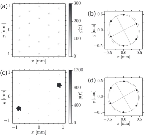
To quantify the deformation of the crystal lattice for the experimental data of Ref. [88], the pair correlation function g(r) in the horizontal plane defined in Eq. 1.32 is considered. The first six peaks of g(r) are fitted to an ellipse centered on the origin. The eccentricity

=p1₋B2

e/A2e of the ellipse, where Ae and Be are the major and minor half axes, is a

measure for the compression of the crystal, and the tilt angleβ between the minor axis and the x-axis denotes the direction of compression.

The synchronization pattern that was observed in Ref. [88] can be described as follows. A line of particles tends to oscillate in synchrony, with a larger oscillation amplitude in the direction perpendicular to the line. The oscillation is in antiphase to the neighboring lines which also oscillate in synchrony, such that a pattern of alternating oscillation is formed. In a hexagonal lattice, the pattern can be oriented in three different directions. A synchronization pattern with the lines along the y-axis and the particles oscillating along the x-axis is sketched in Fig. 2.2. To measure the degree of synchronization in the three directions of the crystal, an orientation-dependent order parameter motivated from the Kuramoto model [114] is proposed. To account for the stripe pattern of alternating phases in complex plasma crystals, a local order parameter is defined as

Ri,θ(t) = 1 Nn

Nn X

j=1

[kjcos(φj,θ−φi,θ)], (2.1)

2.2. Methods 27

θ

=0

i

R

_i,θ

₌₀

=1

y

x

i

R

_i,θ

₌₀

=0

Figure 2.2: Sketch for construction of order parameter. For the calculation of the order parameter in direction θ= 0, the two nearest neighbors of particlei along the y-direction (red circles) are associated with a factorkj= +1, while the other particles (blue circles) have kj=₋1. Counterdirected arrows stand for a phase shift ofπfor the particle oscillations. For two different situation, the resulting order parameter for the central particle i is indicated.

from the projection of the horizontal position in the directionθ. The instantaneous deviation from the time average is obtained with a sliding window of length0.2 s, and the phase is assumed to grow linearly by 2π between each maximum of the deviation. The factor

kj =

(

+1 for particles assumed to be on the same line as particlei

−1 otherwise, (2.2)

determines the sign of the contribution of particle j to the local order parameter. The line with kj = +1 is perpendicular to the direction denoted by the angle θ. As sketched in Fig. 2.2, forθ= 0◦_{, for a particleithe two nearest neighbors along the y-direction contribute}

with a positive factor, while for the other four nearest neighbors, kj=₋1. This leads to a maximal order parameter Ri,θ=0= 1 during a pattern of alternating oscillations as sketched

by the arrows in Fig. 2.2(a). When there is no synchronized pattern as in Fig. 2.2(b), the order parameter averages to zero.

Defects were extensively studied in complex plasmas. In a regular hexagonal lattice, all Voronoi cells are sixfold cells; a defect is then a cell with a different number of faces. Defect chains between domains yield information about structural properties [74, 105, 115]. Gliding dislocations, i. e., isolated pairs of one fivefold and one sevenfold cell, can be used as moving perturbations in the crystal [116]. Here we consider the dislocation dipole vector

d =r7−r5 [117], where r7,5 are the positions of the centers of the sevenfold and fivefold

θ

=0

°

θ

=60

°

θ

=120

°

0

π

2

π

φ

−

1

0

1

R

Figure 2.3: Snapshots of the instantaneous phases and the order parameters during asym-metrically triggered MCI in a simulated crystal. Black dots indicate the particle positions. In the upper line, the instantaneous phases φi,θ of the particle oscillations are shown for the three directions θ= 0◦, 60◦, and 120◦ at time t= 23.87 s. In the lower panels, the associ-ated local order local parameter Ri,θ (see Eq. 2.1) is shown. The crystal was compressed

horizontally under an angle α= 30◦ _{in order to trigger the MCI in the 0}◦ _and60◦ _directions.

See the paper [102] for a similar plot of the experimental data.

2.3

Results

By analyzing the pair correlation function g(r)of the experimental data of Ref. [88], a tilt angle β = 27◦_±2◦ _{and an eccentricity of = 0.42±0.07 were obtained. The crystalline}

lattice was thus clearly compressed. Reasons for an unwanted compression in experiments can be slight anisotropies in the global horizontal confinement or deformations due to the slow horizontal rotation of the crystal during the experiment.

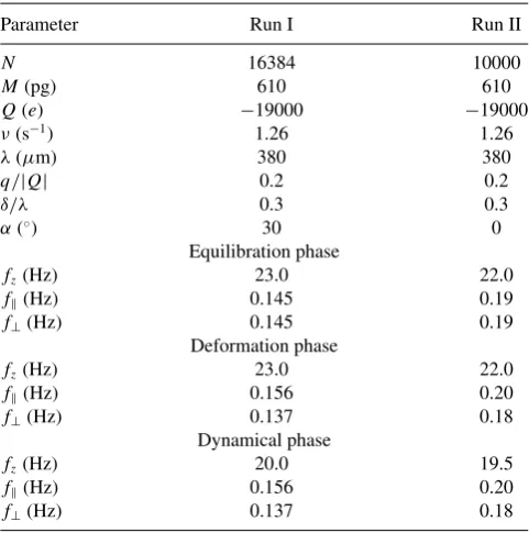
To reproduce the deformed crystal lattice in simulations, an anisotropic horizontal con-finement was considered (see Eq. 1.29) with an angle of α= 30◦ and horizontal confinement frequencies f_k= 0.156 Hz and f_⊥= 0.137 Hz. The anisotropic confinement resulted in a deformed lattice; the ellipse fitted to the first peaks ofg(r)had a tilt angle of β= 29.7◦_±0.5◦

2.3. Results 29

16

18

20

22

x [mm]

-16

-14

-12

-10

-8

y [mm]

12

14

16

18

x [mm]

2

4

6

8

10

y [mm]

a)

b)

Figure 2.4: Defect patterns for simulated (a) and experimental (b) data. The Voronoi cells of particles having more or less than six neighbors are shown in red for fivefold cells, green for sevenfold cells, and gray otherwise. The dislocation dipole vectors d are shown as white arrows. The center of the crystal is located (roughly) at the origin of the coordinate system.

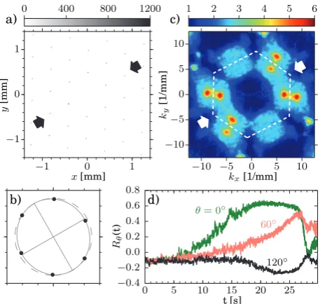
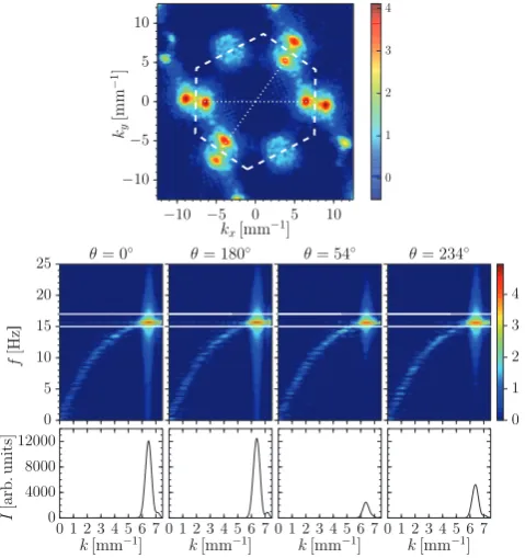
in Fig. 2.1(c), indicate an asymmetric triggering of the MCI in good agreement with the experimental spectra (Fig. 2.1(b)). The compressed crystal lattice allows the MCI to be triggered in the directionsθ= 0◦ _{andθ= 60}◦_{(and the two counterdirected directions θ= 180}◦

and θ= 240◦), while in θ= 120◦ direction no instability is triggered. Recently, the theory of the asymmetric triggering of the MCI was studied by Ivlev et al. by analyzing theoretically the wave modes in a compressed plasma crystal [118].

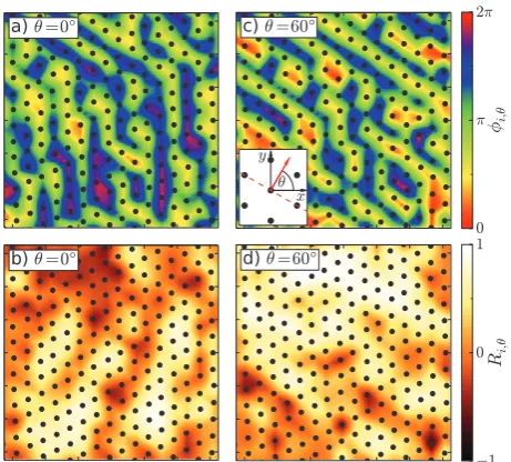
A snapshot of the instantaneous phases φi,θ of the particle oscillations in the three directions θ = 0◦_{, 60}◦_{, and 120}◦ _{is shown in Fig. 2.3 for the simulated crystal during MCI.}

The map of φi,θ=0◦ shows a pronounced pattern with the stripes along they-direction as can be seen in the upper left panel of Fig. 2.3. The map of the corresponding order parameter of Eq. 2.1 (lower left panel) shows values close to unity for almost all particles in the window. Forθ= 60◦_{, the stripes of alternating phases go from the top left to the upper right, and the}

order parameter indicates that synchronization under this angle is most pronounced in the upper region of the window (upper and lower center panels). Finally, when the horizontal trajectories are projected along θ= 120◦_{, as there is no large amplitude associated to MCI}

in this direction, the map of the instantaneous phases looks very similar to the case of

θ= 0◦ _{(compare upper left and upper right panels). The order parameter Ri,θ}

=120◦, however, now shows slightly negative values.

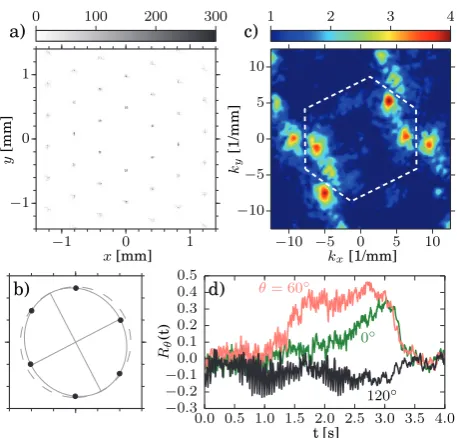
θ= 60◦, the order parameter is positive, while no positive values are obtained in the θ= 120◦ direction. At the beginning of the instability in the experiment, Rθ=60◦ rapidly grows and saturates at R60◦ ' 0.4, while in the other direction R0◦ follows more slowly. The analysis shows that there are two competing synchronization patterns. In the simulation, the dynamics of the order parameters is similar, but the roles of0◦ _and60◦ _{are interchanged.}

In addition, in the experiment the intensities in the 60◦ _{direction and the counterdirected}

240◦ direction are very different (see Fig. 2.1(b)); a similar, but weaker intensity difference can also be observed in the simulations (see Fig. 2.1(c)).

The theory of wave modes in compressed crystals of Ref. [118] cannot explain such a delicate symmetry breaking. From the asymmetric intensity distribution in Fig. 2.1(c) a net phonon flux can be calculated. In the second paper [113], the direction of this flux was calculated to be in the direction of θ = 223◦. Adding a nonvanishing phonon flux in the theoretic calculation of the wave modes indeed reproduces the broken symmetry as can be seen in Figs. 3(d) and 3(e) of the paper [113].

One possible reason for the net phonon flux is phonon scattering by the anisotropi-cally distributed defects in the crystal as indicated by a nonvanishing global dislocation polarization vector D = Pd. In the simulations, a majority of the polarization vectors

d was oriented outward as can be seen in Fig. 2.4(a). In experiments, only the central region of the crystal is observed in order to have a good resolution. In the experimental data considered in the paper, only one major defect line is visible. As can be seen in Fig. 2.4(b), the dislocation vectors are also loosely oriented away from the central region. For an analysis of the global polarization pattern in experiments dedicated studies with a larger field of view would be necessary. A second possible explanation for the net phonon flux is the umklapp scattering which can also happen in a perfect, dislocation-free crystal lattice.

2.4

Conclusion

This chapter focused on symmetry breaking during the mode-coupling instability. By compressing the crystal lattice horizontally, the MCI can be triggered in two or four directions (depending on the angle of compression), in contrast to the triggering of MCI in a perfect hexagonal lattice where all six directions are equally strong. The asymmetric triggering is accompanied by a synchronization pattern or a competition of patterns, which can be characterized by a direction-dependent order parameter.

By repeating the simulations but only taking the linearized interparticle interactions into account, it is possible to discriminate the linear and the nonlinear contributions to the synchronization process. As it is common belief that nonlinear terms are necessary for synchronization to occur, studying synchronization in such a linearized model of the MCI could show that nonreciprocal—but linear—interactions are sufficient, and shed light on the profound properties of synchronization processes [119].

2.4. Conclusion 31

anisotropic phonon scattering at defects and umklapp processes two mechanisms were proposed that could be responsible for the net phonon flux which in turn leads to the broken symmetry.

Chapter 3

Self-propelled motion of an extra

particle

This chapter provides complementary information to the following paper, which appears as Ref. [121] in this thesis.

I. Laut, C. Räth, S. Zhdanov, V. Nosenko, G. Morfill and H. Thomas.

Wake-mediated propulsion of an upstream particle in two-dimensional plasma crystals,

Physical Review Letters118, 075002 (2017)

3.1

Objectives

In 2012, Du et al. observed the intriguing motion of an upstream extra particle moving above the lattice of a two-dimensional plasma crystal [97]. “Extra” means that the particle was not part of the two-dimensional crystal lattice and “upstream” means that the downward ion flow passes by the particle before reaching the crystal. As shown in Fig. 1.7, the particle followed the channel formed by lines of neighboring particles and thus moved in a straight line through the crystal. What is more, the motion of the extra particle was not dampened despite ambient gas friction. It was assumed that the persistent motion was a result of the nonreciprocity of the particle interaction [97, 98], but the exact propulsion mechanism was not explained. The objective of the present work was to reproduce the channeling effect in simulations and study the underlying mechanism in greater detail.

3.2

Methods

To reproduce the channeling effect, the equation of motion Eq. 1.27 is initially integrated for N −1 particles in order to equilibrate the two-dimensional crystal. The crystal is oriented such that the crystal forms channels along the x-direction. After equilibration, the Nth particle, termed extra particle, is added to the crystal at t= 0. Its initial velocity

v(t= 0) =v0ex is oriented in the x-direction. In the experiments, the extra particle was