Efficient Divisor Class Halving on
Genus Two Curves
Peter Birkner?
Department of Mathematics, Technical University of Denmark (DTU) Matematiktorvet, Building 303, DK-2800 Kongens Lyngby, Denmark
Abstract. Efficient halving of divisor classes offers the possibility to improve scalar multiplication on hyperelliptic curves and is also a step towards giving hyperelliptic curve cryptosystems all the features that elliptic curve systems have. We present a halving algorithm for divisor classes of genus 2 curves over finite fields of characteristic 2. We derive explicit halving formulae from a doubling algorithm by reversing this process. A family of binary curves, that are not known to be weak, is covered by the proposed algorithm. Compared to previous known halving algorithms, we achieve a noticeable speed-up for this family of curves.
Keywords.hyperelliptic curve, divisor class halving, binary fields.
1 Introduction
Since hyperelliptic curve cryptosystems (HECC) gain similar attention as their elliptic counterparts, it is very interesting to investigate, whether ideas and methods can be transferred from the elliptic to the hyperelliptic case. The most important operation used by elliptic curve cryptosystems (ECC) is scalar multiplication which is composed of point addition and doubling (when using an double-and-add algorithm) or point addition and halving (when using an half-double-and-add algorithm [7,11]). These operations are well investigated and it is likely that the present formulae are the most efficient ones. For HECC explicit formulae for addition, doubling and hence scalar multiplication of divisor classes are also known [1,8].
Efficient halving of divisor classes offers the possibility to improve scalar multiplication on hyperelliptic curves and is also a step towards giving HECC all the features that ECC have. Halving a divisor class of a hyperelliptic curve is the reverse operation to doubling, i. e. given a divisor class
Done computes another divisor classEsuch that 2E=Dor written in slightly informal notation: 1
2D=E.
In this paper we present an efficient divisor class halving algorithm for hyperelliptic curves of genus 2 over finite fields of characteristic 2. Covering a large family of curves, that are of crypto-graphic interest, the complexity of our algorithm (1I, 8M, 5SR, 2S, 1HT, 1TR)1is only less higher than the complexity of the fastest doubling algorithm (1I, 5M, 6S) for divisor classes [9]. The pro-posed halving method is based on explicit doubling formulae [9] that we use to develop the halving formulae.
The first divisor class halving algorithm for binary curves was proposed by Kitamura, Katagi and Takagi [5,6]. To our knowledge this is the only result on halving of divisor classes so far. Their method covers the general case as well as some exceptional cases which do occur with very low
?Supported by the Danish Research Council for Technology and Production Sciences, grant no. 274-05-0151.
1To describe the complexity of an algorithm we use the following abbreviations: I – Inversion, M – Multiplication, S –
probability. In the general case their complexity is 1I, 18M, 2SR, 2S, 2HT, 2TR in the best case and 1I, 21M, 3SR, 2S, 2HT, 2TR in the worst case.
The special class of curves considered in Appendix D of [6] is covered by our study. However, instead of having a one-parameter family our curves has two free parameters. In the worst case our complexity is 1I, 8M, 5SR, 2S, 1HT, 1TR which is significantly faster even than their formulae.
The remainder of this paper is structured as follows: In the next section we recall some important notions and make a classification of genus 2 curves. In Section 3 we show how we developed the halving formulae by reversing the doubling formulae. The following section contains the actual halving algorithm.
2 Basic Notations and Preliminaries
In this section we briefly recall the definitions of hyperelliptic curves, divisor class groups and the Mumford representation. We also make a classification of hyperelliptic curves over finite fields of characteristic 2 because we focus on a family of curves in this paper. Within the halving algorithm we need to solve a quadratic equation in a finite field of even characteristic. So we will explain how to compute solutions for this at the end of this section.
A comprehensive source for the mathematics of finite fields is [10]. For background on hyperel-liptic curves we refer the interested reader to [1], from which the following definitions and notations are taken.
Definition 1 (Hyperelliptic curve). Let K be a field and let K be the algebraic closure of K. A curve C, given by an equation of the form
C:y2+h(x)y= f(x), (1)
where h∈K[x]is a polynomial of degree at most g and f ∈K[x]is a monic polynomial of degree
2g+1, is called ahyperelliptic curve of genusgoverK if no point on the curve over K satisfies both partial derivatives2y+h=0and f0−h0y=0.
The last condition ensures that the curve is nonsingular. In this paper we concentrate on hyper-elliptic curves of genus 2 over finite fields of characteristic 2. In this case we need a non-zero polynomialhin the curve equation as will be shown now according to [1, p. 309].
Assumingh=0, the partial derivative foryis equal to zero and the one forxis equal to f0(x) =0, which has 2g roots in K. Letx1 be one of them. Then we can find an element y1∈K such that
f(x1) =y21which leads to a singular pointP= (x1,y1)satisfying the curve equation and both partial derivatives. Hence, there is no hyperelliptic curve withh=0 over a field of characteristic 2.
Definition 2 (Divisor class group).Let C be a hyperelliptic curve of genus g over a field K. The group of degree zero divisors of C is denoted byDiv0C. The quotient group ofDiv0Cby the group of
principal divisors of C is called thedivisor class group ofC and is denoted byPic0C. It is also called
thePicard group ofC.
Theorem 1 (Mumford).Let C be a hyperelliptic curve of genus g over an arbitrary field K. Each nontrivial divisor class of C over K can be represented by a unique pair of polynomials u,v∈K[x], where
3. u|v2+vh−f .
Our proposed halving algorithm in Section 4 expects the input divisor class to be in Mumford representation and works directly on the coefficients of the polynomials u and v. The resulting divisor class is also given in the Mumford form.
2.1 Classification of Genus Two Curves
In this paper we deal with hyperelliptic curves of genus 2 overF2d. To avoid Weil descent attacks
[4] one usually restricts to prime degree field extensions for cryptographic applications. So in the following we particularly assume d to be odd.
The genus 2 curves overF2d can be sorted into three different categories depending on the
2-rank of the divisor class group of the curve (see [3]). All pointsPin the support of a divisor class of order 2 satisfyP=ι(P), whereι is the hyperelliptic involution. IfP= (x,y)is not the point at infinity, its coordinates must satisfyy=h(x) +y. So,xis a root ofh(x)and we have that the degree ofhequals the 2-rank of Pic0C. In this paper we focus on curves whose divisor class group has 2-rank equal to one, i. e. in the curve equation we have degh=1. In [2,1] these curves are called curves of Type II. Over a fieldF2d withdodd, one can perform the following transformations
x7→µ2x0+λ and y7→µ5y0+µ4αx02+µ2βx0+γ,
where µ is such that µ3=h1, λ =h0h−11, α =pλ+f4, β a root ofx2+h1x+f2+f3λ+εh21 withε=Tr (f2+f3λ)h−12andγ= (λ2f3+λ4+f1)h−11, to obtain a unique representative of each isomorphism class given by
C:y2+xy=x5+f3x3+f2x2+f0, (2)
where f2∈F2andf0,f3∈F2d[1, Proposition 14.37]. So, for the remainder of this paper we consider
(2) as a Type II curve.
Since f2∈F2, we have 2·2d·2d =22d+1 different choices for the right-hand side of (2), i. e. Type II covers (up to isomorphism) 22d+1 different curves of genus 2 where our halving algorithm can be applied.
2.2 Quadratic Equations inF2d
In the halving algorithm we need to solve a quadratic equation inF2d. Provided a solution exists,
we can use a simple formula to compute it.
Consider the quadratic equationX2+aX+b=0 over the finite fieldF2d. By substitutingXby X/a, one gets the simpler equation
T2+T =c, withc=b/a2, (3)
which has a solution in the fieldF2d if and only if the trace ofcis equal to zero [1, Section 11.2.6].
Ifdis odd, then a solution of (3) is given by
t=
(d−3)/2
∑
i=0
c22i+1. (4)
2.3 Choice of the Field Representation
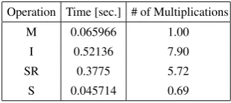
Like in the doubling formulae we have to compute inversions, multiplications and squarings to halve a divisor class. Additionally we need to be able to efficiently compute square roots, traces and half-traces. In order to speed these operations up, one can use a normal basis representation. Having this we can compute the square of a field element simply by shifting the representing vector. Computing a square root works the same way but shifting to the opposite direction. Because traces and half-traces are sums of powers of squares, they can be calculated very efficiently, too. In a hardware implementation, multiplications and inversions in the field can be hard-coded in order to get best performance.
Software libraries like NTL work with a polynomial basis representation and do not provide efficient square root computations in characteristic two. So, we implemented our own square root function for the finite fieldF283and present some timings for field operations. We used the Number
Theory Library (NTL 5.4) together with the GNU Multiple Precision Arithmetic Library (GMP 4.2.1) and the GNU Compiler Collection (GCC 4.0.1) on an Apple MacBook with a 2,0 GHz Intel Dual Core CPU to compute the benchmarks. The multiplication, inversion and squaring functions are taken from NTL, the square root function is our own implementation for that particular finite field. We measured the time for 100,000 operations each.
Operation Time [sec.] # of Multiplications
M 0.065966 1.00
I 0.52136 7.90
SR 0.3775 5.72
S 0.045714 0.69
Table 1.Timings of field operations inF283
3 From Doubling to Halving
In this section we derive the halving formulae from the doubling formulae. Therefore, we present first how to double a divisor class given in Mumford representation using explicit formulae. Then we explain how we found the halving formulae by reversing the doubling algorithm.
In the entire section we assumeCto be a Type II hyperelliptic curve of genus 2 overF2d, where d is odd, given by equation (2). In the following we also need to assume that the group order of PicC0(F2d) is 2r, where r is odd.2 For cryptographic applications one wants to work in a cyclic
subgroup of prime orderl. So we denote the orderl-subgroup of PicC0(F2d) byS. Note, however,
that the following considerations also hold muta mutandis in the subgroup of orderr.
3.1 Doubling of Divisor Classes
LetE= [x2+u01x+u00,v01x+v00]be a divisor class in the orderl-subgroupSof Pic0C(F2d). Becausel
is prime, there exists no proper subgroup ofSand hence it is cyclic. So, each divisor class contained inSis the double of another divisor class in the same subgroup, i. e. each divisor class inScan be
doubled and hence also be halved. In [5] the elements of this subgroup are calledproper divisor classes.
We can compute the doubled divisor classD=2E= [x2+u1x+u0,v1x+v0]using Lange and Steven’s explicit formulae (see [9]):
u1= u 0
0 2
f0+v002
!2
, (5)
u0=
u012+f3
u0
0 2
f0+v00 2
! +u01
!2
+ u
0
0 2
f0+v00 2
!
, (6)
v0=
u002
f0+v00
2+u
0
1 2
+f3
! u0+u00
2
, (7)
v1=
u002
f0+v002
+u012+f3
!
u012+f3
u0
0 2
f0+v002
!
+ u
0
0 2
f0+v002
!
u1+f2+v01 2
. (8)
Notice that we are considering a curve of form (2), i. e.h(x) =x. Hence, the coefficienth1occurring in Lange and Steven’s formulae equals one and does not appear here.
3.2 Halving of Divisor Classes
Now, we turn around and compute the half of a divisor class by applying the doubling formulae in reverse order. Given a divisor classD= [x2+u1x+u0,v1x+v0], we show how to compute a divisor classE = [x2+u01x+u00,v01x+v00]such thatD=2E. Therefore, we need again to say thatDmust be contained in the orderl-subgroupSof Pic0C(F2d)in order to ensure that the double and the half
of each divisor class does exist in this particular subgroup. Taking√u1from (5), we can writeu0using (6) as
u0=
(u012+f3)
√
u1+u01
2
+√u1. (9)
Now, using the fact that we are in characteristic 2 we can expand the quadratic expression and arrange the terms such that we get a quartic equation inu01on the right-hand side:
u0=u014u1+u012+ f32u1+√u1. (10)
SubstitutingU=u012yields a quadratic equation in the variableU:
U2u1+U=u0+f32u1+
√
u1. (11)
Multiplying both sides by u1 and substituting T =U·u1 afterwards yields a quadratic equation
T2+T =cwherec=u1u0+f32u21+u1
√
u1like (3).
Because Dis an element of the subgroup S, there exists an elementE ∈S with D=2E. So
that the trace ofcis equal to zero. We also know that there exist two solutionstandt+1 which can be computed using (4). After adjusting these two solutions by dividing byu1we have two solutions of (11). Re-substitutingu01=pt/u1 oru01=
p
(t+1)/u1 respectively yields two possible values foru01in (10). We will show how to figure out which of these two solutions is the right one at the end of this section. For now let us suppose that we already know the correctu01.
Takingv0from (7) and writing again u
0 0 2
f0+v00 2 as
√
u1, we obtain:
v0=
√ u1+u01
2
+f3
u0+u00
2
, (12)
which leads us to a new expression foru00using the already known valueu01:
u00= r
v0+√u1+u102+f3u0. (13)
Now we are able to computev00usingu00and (5):
v00= s
u002
√
u1
+f0. (14)
The last step is to computev01using (8):
v01= r
v1+
√
u1
(√u1+u012+f3)(u012+f3) +u1
+f2. (15)
Let us now come back to figuring out which of the two solutions of the quadratic equationT2+ T =c is the right one. In order to do that, we use the first solution t and continue computing the halved divisor class as explained above. If this choice was correct, then the halved divisor class is a proper one, i. e. it is contained in the subgroupS. So we have to check this. As we have seen above, the trace ofc=u21
u0
u1+f
2 3+ √ u1 u1
=u1 u0+u1f32+
√
u1
is zero if and only if the divisor class is contained in S. We now check if the obtained divisor class can be halved, i. e. whether Tr u01(u00+u10 f32+pu01)
=0.If this holds, then the first solutiont was correct and we have computed the correct halved divisor class. If the trace is not zero, we use the other solution
t+1 of the quadratic equation. So the trace serves as a criteria to determine the right solution of (11). Note, that this test involves computingu01 andu00. So it should be performed as soon as they are computed. If the other solution turns out to be the correct one, we have to redo the computation ofu01andu00usingt+1 instead oft.
After computingu01,u00,v01andv00we can write the halved divisor class in Mumford representa-tion:E= [x2+u01x+u00,v01x+v00].
3.3 The Caseu1=0
The formulae presented in the previous section hold in the generic case, i. e. if both the input and output haveuandvof full degree and no zero coefficients. To complete the above study we now consider how to compute the half of a divisor class withu1=0.
We now consider the divisor classD= [x2+u0,v1x+v0], whereu1equals zero. From equation (5) follows directlyu00=0. Using this and equation (6) we getu0=u012and hence,u01=
√
u0. This shrinks (8) tov1= f2+v012 and we havev01=
√
v1+f2. Havingu00=0, one can see that the four equations (5), (6), (7) and (8) do not depend onv00any longer, so this value becomes arbitrary. So, (14) should not be performed.
The complete procedure explained above leads to the actual halving algorithm presented in the next section.
4 The Divisor Class Halving Algorithm
We present an efficient divisor class halving algorithm for genus 2 curves of Type II (cf. Section 2.1) overF2d, whered is odd, based on the formulae derived in the previous section. We do not
follow the steps literally but change them to allow more efficient computations.
We shortly repeat the prerequisites: The curve parameters must be chosen such that the order of PicC0(F2d)is equal to 2rfor an odd numberr. The input divisor class must be contained in the order l-subgroup of PicC0(F2d), wherelis prime.
Algorithm 1Divisor Class Halving (HLV)
INPUT: Divisor classD= [u,v], whereu=x2+u1x+u0,v=v1x+v0and the
pre-computed valuesf32,√f0
OUTPUT: Halved divisor classE= [u0,v0]such thatD=2E
1: q1←√u1,q2←1/q1,q3←q22,q4←u0q3,q5←
√
q2 .1I, 1M, 2SR, 1S
2: q6←
√
q4,c←u1(q6+q5+f3) .1SR, 1M
3: t0← (d−3)/2
∑ i=0
c2(2i+1) .1HT
4: u01←t0q2,t←u012,s1←v0+ (q1+t+f3)u0 .2M, 1S
5: u00←√s1,b←Trace(u01(u00+t+f3)) .1M, 1SR, 1TR
6: ifb=0 then
7: v00←q5u00+
√
f0 .1M
8: else
9: t←t+q3,u01←u01+q2
10: u00←u00+q6,v00←q5u00+
√
f0 .1M
11: end if
12: v01←
r
v1+q1
(q1+t+f3)(t+f3) +u1
+f2 .2M, 1SR
13: return[x2+u01x+u00,v01x+v00] .Total: 1I, 8M, 5SR, 2S, 1HT, 1TR
We now explain the steps of the algorithm according to the formulae derived in the previous section.
Some expressions in the halving formulae do occur more than once. To avoid recomputations, we replace them by q1, . . . ,q6 in Step 1 and 2. To solve the quadratic equation (11) we have to computeu1(u0+u1f32+
√
u1). What we actually do in the algorithm is computingu1(q6+f3+q5) which is the square root ofu1(u0+u1f32+√u1)and use that Tr(a2) =Tr(a)for anya∈F2d. The
According to the explanation at the end of the previous section, we now have to compute the trace ofu01(u00+pu01+u01f32)in order to perform the check whether we calculated the right solution of the quadratic equation or not. To reduce the number of operations we compute the trace of
u01(u00+t+f3)instead. Doing this saves 1M, 1SR and 1S. To see that these two traces are equal, we point out that Tr(u01pu01) =Tr(u01t), Tr(u012f32) =Tr(u01f3)and that the trace is a linear map.
In Steps 6 to 11 we compute v00 depending on the trace b. If this trace is equal to zero, we continue by computingv00using (14). Forb=1 we uset0+1 instead oft0in Step 3. Hence, we have to adjustxby addingq3,u01by addingq2andu00by addingq6in Steps 9 and 10. After that we can computev00in the same way as in Step 7.
The last thing to do is computing v01 using (15) in Step 12. Finally the algorithm returns the desired halved divisor class in Mumford representation. The steps, considered so far, have a total complexity of 1I, 8M, 5SR, 2S, 1HT, 1TR in both casesb=1 andb=0.
5 Conclusion and Outlook
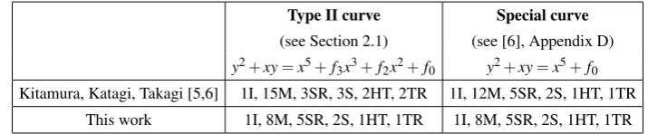
In this paper we presented an efficient halving algorithm for divisor classes of a family of hyper-elliptic curves of genus 2 over binary fields. Compared to the previous result by Kitamura, Katagi and Takagi [5,6] we gained a notable speed-up for this family (see Table 2).
In Appendix D of [6] the authors consider curves of form
y2+xy=x5+f1x+f0.
The transformationy7→y˜+f1 maps to the isomorphic curve ˜y2+xy˜=x5+f˜0, which is a Type II curve. This equation shows that their family of curves has only one parameter that can be chosen freely while our family achieves full generality for Type II curves needing far less operations (cf. Table 2).
Type II curve Special curve
(see Section 2.1) (see [6], Appendix D)
y2+xy=x5+f3x3+f2x2+f0 y2+xy=x5+f0
Kitamura, Katagi, Takagi [5,6] 1I, 15M, 3SR, 3S, 2HT, 2TR 1I, 12M, 5SR, 2S, 1HT, 1TR This work 1I, 8M, 5SR, 2S, 1HT, 1TR 1I, 8M, 5SR, 2S, 1HT, 1TR
Table 2.Complexity of halving algorithms in worst case
We would like to point out that we can improve the efficiency of our algorithm as well as that of doubling by leaving out the computation ofv1in a Montgomery like scalar multiplication, since the new valuesu0,u1andv0do not depend on it. We are investigating the required addition formulae.
References
1. Roberto Avanzi, Henri Cohen, Christophe Doche, Gerhard Frey, Tanja Lange, Kim Nguyen, and Frederik Ver-cauteren.The Handbook of Elliptic and Hyperelliptic Curve Cryptography. CRC Press, 2005.
2. Bertrand Byramjee and Sylvain Duqesne. Classification of genus 2 curves overF2nand optimization of their
3. YoungJu Choie and Dong Kyun Yun. Isomorphism Classes of Hyperelliptic Curves of Genus 2 overFq. In Infor-mation Security and Privacy – ACISP 2002, volume 2384 ofLecture Notes in Computer Science, pages 190–202. Springer-Verlag, 2002.
4. Pierrick Gaudry, Florian Hess, and Nigel P. Smart. Constructive and destructive facets of Weil descent on elliptic curves.Journal of Cryptology, 15(1):19–46, 2002.
5. Izuru Kitamura, Masanobu Katagi, and Tsuyoshi Takagi. A Complete Divisor Class Halving Algorithm for Hyper-elliptic Curve Cryptosystems of Genus Two. InInformation Security and Privacy – ACISP 2005, volume 3574 of
Lecture Notes in Computer Science, pages 146–157. Springer-Verlag, 2005. (for a full version see [6]).
6. Izuru Kitamura, Masanobu Katagi, and Tsuyoshi Takagi. A Complete Divisor Class Halving Algorithm for Hyper-elliptic Curve Cryptosystems of Genus Two.Cryptology ePrint Archive of IACR, Report 2004/255, 2005.
7. Erik Woodward Knudsen. Elliptic Scalar Multiplication Using Point Halving. InASIACRYPT’99, volume 1716 of
Lecture Notes in Computer Science, pages 135–149. Springer-Verlag, 1999.
8. Tanja Lange. Formulae for Arithmetic on Genus 2 Hyperelliptic Curves. Applicable Algebra in Engineering, Communication and Computing, 15(5):295–328, 2005.
9. Tanja Lange and Marc Stevens. Efficient Doubling for Genus Two Curves over Binary Fields. InSelected Areas in Cryptography – SAC 2004, volume 3357 ofLecture Notes in Computer Science, pages 170–181. Springer-Verlag, 2005.
10. Rudolf Lidl and Harald Niederreiter.Finite Fields, volume 20 ofEncyclopedia of Mathematics and its Applications. Addison-Wesley, 1983.
11. Richard Schroeppel. Elliptic curve point halving wins big. 2nd Midwest Arithmetical Geometry in Cryptography Workshop, Urbana, Illinois, November 2000.
A Magma Implementation of the HLV Algorithm
Here is a sample Magma implementation of the HLV algorithm for the finite fieldF27.
GF2 := FiniteField(2); R_GF2<z> := PolynomialRing(GF2);
F := ext < GF2 | z^7 + z + 1 >; // Define the extension field F_{2^7} R<x> := PolynomialRing(F);
f0 := F.1^41; // Setup the curve parameters f2 := 1; //
f3 := F.1^32; //
f := x^5 + f3*x^3 + f2*x^2 + f0; // Curve equation: y^2 + h(x)y = f(x) h := x; //
C := HyperellipticCurve(f, h); J := Jacobian(C);
r := #J; // Compute the order of the Jacobian
halving := function(D)
u0 := Coefficient(D[1], 0); u1 := Coefficient(D[1], 1); v0 := Coefficient(D[2], 0); v1 := Coefficient(D[2], 1);
q1 := Sqrt(u1); q2 := 1 / q1; q3 := q2^2; q4 := u0 * q3; q5 := Sqrt(q2); q6 := Sqrt(q4);
c := u1 * (q6 + q5 + f3);
xp := &+[c^2^(2*i + 1) : i in [0..2]];
u1p := xp*q2; x := u1p^2;
t := Trace(u1p * (u0p + x + f3));
if (t eq 0) then
v0p := q5 * u0p + Sqrt(f0); else
x := x + q3; u1p := u1p + q2; u0p := u0p + q6;
v0p := q5 * u0p + Sqrt(f0); end if;
v1p := Sqrt(v1 + q1 * ((q1 + x + f3) * (x + f3) + u1) + f2);
return [u1p, u0p, v1p, v0p]; end function;
// Now define a sample divisor class and compare D, 2D and the half of 2D D := J ! [x^2 + F.1^18*x + F.1^80, F.1^17*x + F.1^117];