Article
1
Improving the Accuracy in Text Classification
2
Methodology in Light of Modelling the Latent
3
Semantic Relations
4
Nina Rizun1, Yurii Taranenko 2 and Wojciech Waloszek 3,*
5
1 Gdansk University of Technology; [email protected]
6
2 Alfred Nobel University, Dnipro; [email protected]
7
3 Gdansk University of Technology; [email protected]
8
9
* Correspondence: [email protected]; Tel.: +48-575-434-778
10
† This manuscript is an extended version of our paper “The Algorithm of Modelling and Analysis
11
of Latent Semantic Relations: Linear Algebra vs. Probabilistic Topic Models” published in the
12
proceedings of Knowledge Engineering and Semantic Web, Szczecin, Poland, 8–10 November
13
2017
14
15
Abstract: The research presents the Methodology of Improving the Accuracy in Text Classification
16
in Light of Modelling the Latent Semantic Relations (LSR). The aim of this Methodology is to find
17
the ways of eliminating the Limitations of Discriminant and Probabilistic methods for LSR revealing
18
and customizing the Text Classification Process to the more accurate recognition of the text tonality.
19
This aim should be achieved by using the knowledge about the text’s Hierarchical Semantic Context
20
in the form of Corpora-based Hierarchical Sentiment Dictionary. The main scientific contribution of
21
this research is the following set of approaches to improve the qualitative characteristics of Text
22
Classification process: combination of the Discriminant and Probabilistic methods allowing to
23
decrease the influences of the Limitations of these methods on the LSR revealing process;
24
considering each document as a complex structure allowing to estimate documents integrally by
25
separated classification of topically completed textual component (paragraphs); taking into account
26
the features of Argumentative type of documents (Reviews) allowing to use the author’s subjective
27
evaluation of text tonality for development the Text Classification methodology. Tonality, expressed
28
by the Review’s author, has a significant, but not critical, effect on the qualitative indicators of
29
Sentiment Recognition.
30
Keywords: Text Classification; Topic Modelling; Latent Semantic Analysis; Latent Dirichlet
31
Allocation; Hierarchical Sentiment Dictionary, Contextually-Oriented Hierarchical Corpus; Text
32
Tonality; Evaluation
33
34
1. Introduction
35
The rapid development of computer technology and the Internet space in recent decades has led
36
to the fact that the procedures for creating and accessing the information content of many web
37
resources have become an integral part of private and professional activities of a person. The content
38
of information resources such as social networks, feedback services, web forums and blogs, is actively
39
formed by the users themselves and is publicly available.
40
On the other hand, this content, as well as some more official information (for example, financial
41
statements of enterprises, scientific and news articles) forms a large array of unstructured text
42
information containing a huge amount of Explicit and Hidden knowledge.
43
One of these types of knowledge is the Latent Semantic Relations (LSR), hidden both inside the
44
documents and between them in order to identify the context of the analyzed document, as well as
45
to classify a group of documents based on their semantic proximity. Modelling and Analysis of Latent
46
Semantic Relations (LSR) – is the approach of constructing a model, reflecting the transition from a
47
set of documents and set of words in the documents to a set of topics, describing the contents of
48
documents. We can say that in the mathematical model of text collection, describing the words or
49
documents is associated with a family of probability distributions on a variety of topics [1, 2, 3].
50
In addition to the Latent Semantic analysis, an important task of the classification of texts is to
51
identify their emotional coloring. A special section of computer linguistics is devoted to extraction of
52
such information – automatic analysis of text tonality (Sentiment Analysis or Opinion Mining) [4].
53
The initial goal of Sentiment analysis methods was classification of documents, and later of sentences,
54
according to a given scale of tonality, usually a two-point negative) or three-point
(positive-55
negative-neutral). However, instead of a general assessment of tonality, a more detailed study of the
56
expressed views on specific aspects (contexts) is required. Therefore, over time, the initial formulation
57
of the task of tonality analysis has acquired a more detailed formulation and has emerged as a
58
separate problem of contextually-oriented sentiment analysis, which is to automatically determine
59
the views of the user, expressed in the text, with respect to specific aspects being examined.
60
This research is devoted to finding ways of Improving the Accuracy in Text Classification via
61
effective implementation of Modelling the Latent Semantic Relations approaches for extracting the
62
knowledge about the documents Semantic Context and further representation, and using this
63
knowledge in the form of Corpora-based Hierarchical Contextually-Oriented Sentiment Dictionary.
64
This paper is an extended version of [5], and the following section were added:
65
extended version of Case Study Results and Discussion section for Latent Semantic Relations
66
Revealing Phase;
67
representation of the new stage of research, based on the results obtained in the paper [5]. In this
68
regard, a new section has been added describing the methodological and experimental parts of
69
the Phase of Text Classification Based on the Contextually-Oriented Sentiment Dictionary.
70
2. Theoretical Background of the Research
71
2.1. Vector Space Models of the Semantic Relations Analysis
72
The aim of the LSR analysis is to extract "semantic structure" of the collection of information
73
flow and automatically expands them into the underlying topic. Significant progress on the problem
74
of presenting and analyzing the data has been made by researchers in the field of information
75
retrieval (IR) [6-8]. The basic methodology proposed by IR researchers for text collection reduces each
76
document in the corpus to a vector of real numbers, each of them representing ratios of counts.
77
In the popular TFIDF scheme [9-13], on the basis of vocabulary of “bag of words” the
78
) (m n
A terms-document matrix is built, which contains (as elements) the counts of absolute
79
frequency of words occurrence. After suitable normalization, this term frequency count is compared
80
to an inverse document frequency count, which measures the number of occurrences of a word in the
81
entire corpus:
82
df
D
t
w
tf
IDF
TF
F
wi
(
,
)
log
2
, (1)
where,
tf
(
w
,
t
)
– relative frequency of the wth word occurrence in document t:83
df
t
w
k
t
w
tf
(
,
)
(
,
)
, (2))
,
(
w
L
tk
– the number of wth word occurrences in the text t;df
– total number of words in the84
Then, for solving the problem of finding the similarity of documents (terms) from the point of
86
view of their relation to the same topic, different metric can be applied. The most appropriate metric
87
is cosine measure of the edge between the vectors:
88
y x
y x dist
i
t
cos , (3)
where xy – scalar product of the vectors,
x
andy
– quota of the vectors, which are89
calculated by the formulas:
90
n
i i
i n
i i
i y y
x x
1 2
1 2
, , (4)
Further part of the algorithm is to divide the source data into groups corresponding to the events,
91
as well as to determine whether a text document describes a set of any topic. The main idea of the
92
solution is the use of clustering algorithms [3, 14, 9-13].
93
The limitations of this method are: the calculations measure the "surface" usage of words as
94
patterns of letters; they can't distinguish such phenomena as polysemy and synonymy [3, 7, 15].
95
2.2. Latent Semantic Indexing
96
In 1988, Dumais et al. [16] proposed a method of Latent Semantic Indexing (LSI), most frequently
97
referred to as LSA. Deerwester et al. in 1990 [17], designed to improve the efficiency of IR algorithms
98
and search engines by projection of documents and terms in the space of lower dimension, which
99
includes semantic concepts of the original set of documents.
100
LSA is a matrix algebra process. The most common version of LSA is based on the singular value
101
decomposition (SVD) of a term-document matrix [7]. As a result of the SVD of the matrix A we have
102
three matrices:
103
T K K K Kd
t
X
tdU
td tdV
tdX
, (5)
T K Ktd V td – represents terms in k-d latent space;
d t d t K
K
U
– represents documents in k-d
104
latent space; d t
K
U
, VKtd – retain term–topic, document–topic relations for top k topics.
105
But, as [9, 10] proved, there are three limitations to apply LSA: documents having the same
106
writing style (Lim#1); each document being centered on a single topic (Lim#2); a word having a high
107
probability of belonging to one topic but low probability of belonging to other topics (Lim#3). The
108
limitations of LSA are based on orthogonal characteristics of dimension factors as well as on the fact
109
that the probabilities for each topic and the document are distributed uniformly, which does not
110
correspond to the actual characteristics of the collections of documents [16, 17, 18]. That is why, LSA
111
tends to prevents multiple occurrences of a word in different topics and thus LSA cannot be used
112
effectively to resolve polysemy issues (Lim#4).
113
2.3. Probabilistic Topic Models
114
In contrast to the so-called discriminative approaches (LSI, LSA), in a probabilistic approach the
115
topics are given by the model, and then term-document matrix is used to estimate its hidden
116
parameters, which can then be used to generate the simulated distributions [4, 6, 17, 24].
117
2.3.1. Latent Dirichlet Allocation
118
LDA – generative probabilistic graphical model proposed by David Blei [1, 2, 15]. LDA is a
three-119
level hierarchical Bayesian model. The algorithm of the method is as follows: Each document is
120
generated independently: randomly select its distribution for document on topics
d for each word121
select a word from the distribution of words in the chosen topic
k( distribution of words in the123
topic k). In the classical model of LDA the number of topics is initially fixed and specifies the explicit
124
parameter k.
125
2.3.2. Methods of Evaluating the Quality of Results
126
The most common method of evaluating the quality of probabilistic topic models is calculation
127
of the Perplexity index on the test data set
D
test [1, 2, 20, 21]. In information theory, perplexity is a128
measurement of how well a probability model predicts a sample. Low perplexity indicates that the
129
probability distribution is good at predicting the sample:
130
M
d d
M
d d
test
N w p D
Perplexity
1
1log ( )
exp
( , (6)
The limitation of LDA method is: it is possible to choose the optimum value of the k but, even
131
under condition of finding the optimal value of the k, the level of probability of a document belonging
132
to a particular topic could be insignificant (Lim#5) [1, 2, 22].
133
2.4. Textual Content Classification
134
Methods of contextually-emotional analysis of the text are developed within the framework of
135
two machine learning approaches: supervised and unsupervised machine learning [4]. In the
136
approach based on supervised machine learning, a marked collection of documents is needed, which
137
lists examples of emotional expressions and aspect terms.
138
The methods of unsupervised machine learning allow to avoid dependence on training data. For
139
their work, one also needs a Corpus of documents, but preliminary markup is not required. Within
140
the framework of this approach, the probabilistic-statistical regularities of the text are found and, on
141
their basis, the key subtasks of the aspect-emotional analysis are solved: identification of aspect terms
142
and determination of their tonality. However, such methods require complex tuning to a given
143
domain. For example, the method based on Latent Dirichlet Allocation (LDA) in its original form is
144
not able to effectively detect topics, therefore, its additional adaptation and adjustment of
145
correspondence of identified topics to the target set of contexts is required [23].
146
The methods of Text Classification, considered above, require the presence of Sentiment
147
Dictionary of text tonality evaluation. There are three basic approaches to such Dictionary [4]: expert;
148
based on dictionaries / thesaurus; and on the basis of text collections.
149
With the expert approach, the dictionary is compiled by experts. The approach differs, on the
150
one hand, by complexity and high probability of the absence of domain-specific words in the
151
dictionary, on the other – by high quality of the dictionary in sense of adequacy of the assigned key.
152
In the dictionaries / thesaurus approach, the initial small list of evaluation words is expanded by
153
various dictionaries, for example, explanatory or synonyms / antonyms. This also does not take into
154
account the subject area.
155
In the approach based on text collections, statistical analysis of the marked texts, as a rule,
156
belonging to the subject domain in question, is used to compile the Dictionary.
157
In [24], the dictionary of emotional vocabulary, compiled by experts manually, was used to
158
determine the tone of individual words. In the dictionary, each word and phrase are associated with
159
orientation of the key (positive / negative) and with strength (in points).
160
The author's methods proposed in [25, 26] are based on a dictionary approach: to determine the
161
tonality of texts, a dictionary of estimated words is used, where each word has a numerical weight
162
that determines the degree of word significance. In the method of working with the dictionary closest
163
to the paper [27]), however: the dictionary firstly is created on the basis of a statistical analysis of
164
training collection; secondly, the weight of words is determined with the help of a genetic algorithm.
165
In most studies, tone of the text is determined on the basis of calculation of weights of the
166
C
N
i i С
T
w
W
1, (7)
where
W
TС – weight of text T for tonality C; wi – weight of the evaluated word i; NC – number168
of estimated bigrams of tonality C in the text T.
169
To classify texts according to the linear function:
170
negT neg pos T neg T pos
T
W
W
k
W
W
f
,
, (8)
where
W
Tposis the positive weight of the text T;W
Tnegis the negative weight of the text T;k
neg171
is the coefficient compensating the fact of preponderance of positive vocabulary in text [28]. If the
172
value of the function f is greater than zero, the text is positive, otherwise – negative.
173
3. Methodology
174
In this paper the following author’s definitions will be used:
175
1. Term is a basic unit of discrete data.
176
2. Contextual Fragment (CF) is an indivisible, topically completed sequence of terms, located within
177
a document’s paragraph.
178
3. Document is a set of CF.
179
4. Corpus (films reviews corpus, FRC) is a collection of Documents.
180
5. Topic is the Label (one term) that defines the main semantic context of the CF.
181
6. Contextual Dictionary (CD) is a set of key words that describe semantic context of the Topic.
182
7. Semantic Cluster (SC) is the set of CF that have hidden semantic closeness (HSC).
183
8. Contextually-Oriented Corpus (HC) is a Hierarchical structure of semantically closes CF, built via
184
application of unsupervised machine learning Discriminant and Probabilistic Methods of the
185
Topic Modelling and Latent Semantic Relations Analysis.
186
9. Corpora-based Sentiment Dictionary (CBSD) is a Manually Created Dictionary, which has Semantic
187
and Hierarchical Structure thanks to using the Contextually-Oriented Corpus for its building.
188
3.1. Novelty and Motivation
189
Motivation scenario of this research presupposes taking into account the Specificity of the
190
analyzed Document Type and concerns finding the ways to completely or partially:
191
Eliminate the Limitations characterizing the Discriminant and Probabilistic approaches for
192
Latent Semantic Relations revealing;
193
Customize the Text Classification Process to the more accurate recognition of the text tonality in
194
light of Semantic Context of the topic.
195
In this regard the following scientific research questions (RQ) were raised:
196
RQ_1. Whether taking into account the specific features of Argumentative/ Persuasive type of
197
document allows to affect Quality of the Topic Modelling Process Results.
198
RQ_2. Is it possible to increase the Level of Quality of the Topic Modelling Process Results via
199
using the combination of the Discriminant and Probabilistic Methods?
200
RQ_3. Whether taking into account Hierarchical structure of Latent Semantic Relations within
201
the Corpus allows to affect Accuracy of the Text Classification Results.
202
RQ_4. Is it possible to increase the Text Classification Process Accuracy via building and using
203
the Contextually-Oriented and Semantically Structured Sentiment Dictionary?
204
For finding the answers to these questions the following main Assumptions (A) were formulated:
205
A1. Taking into account the specificity of Type of Documents, chosen for this study, and presence
206
of the nonofficial requirements of Film’s Review structure and writing rules [29], assume that the
207
A2. Taking into account the chosen Document Type Specificity, assume that each document has
209
a complex structure and can be estimated integrally by separated classification of topically completed
210
textual component (paragraphs), centered on a single Topic, as elements of their structure
211
(eliminating the Lim#2).
212
On the basis of the research questions and proposals raised, the following scientific Hypotheses
213
(H) were formulated:
214
H1. Combination of the unsupervised machine learning Discriminant and Probabilistic methods
215
has a synergistic effect to improve the recall rate and precision indicator of Topic Modelling Process
216
realization. This effect is expected to be achieved via increasing:
217
Quality of LDA-method of topics recognizing via increasing the level of probability of assigning
218
the topic to particular CF by taking into account the hidden LSR phenomena (eliminating the
219
Lim#5);
220
Quality of LSA-method of LSR recognition via adjusting the consequences of influence of the
221
uniform distribution of the topics within the document by taking into account the probabilistic
222
approaches (eliminating the Lim#3 and #4).
223
H2. Identifying and taking into account the Hierarchical structure of Latent Semantic Relations
224
within the Corpus effect to improve the Text Classification Process Accuracy. This effect is expected
225
to be achieved via increasing:
226
Adequacy of Tonality Assessment Instruments via building the Manually Creating Hierarchical
227
Contextually-Oriented and Semantically Structured Corpora-based Sentiment Dictionary;
228
Quality of the Sentiment Analysis results via adjusting the Algorithms of using the Tonality
229
Assessment Instruments by applying integral evaluation of its individual topically-oriented
230
fragments using the CBSD and taking into account the tonality, subjectively assigned to texts by
231
the author.
232
Proposed Methodology of Improving the Accuracy of Text Classification based on revealing and
233
using the knowledge about Latent Semantic Relations includes 2 main phases:
234
Latent Semantic Relations revealing Phase;
235
Text Classification based on the CBSD Phase.
236
As a sample for case study experiments the Polish-language film reviews dataset from the
237
filmweb.pl was used. The experimental part of author's Methodology has been implemented in
238
Python 3.4.1.
239
3.2. Latent Semantic Relations Revealing Phase
240
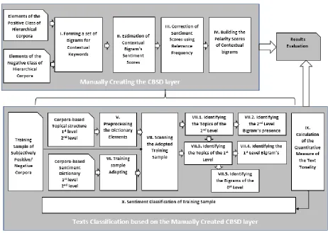
Basic version of Latent Semantic Relations RevealingPhaseincludes 7 steps (figure 1).
241
3.1.1. LDA-based Analyzing of Latent Semantic Relations Layer
242
Step I. Identifying the Topics
243
LDA-based Analysis of LSR is the layer, which aims:
244
1. To reveal the optimal number of latent probabilistic topics that describe the main content of the
245
analyzed document;
246
2. To assign them to the CFs based on the probabilistic LSR within the paragraphs.
247
As a technical support, for the implementation this phase the LDA Genism Python package
248
(https://radimrehurek.com/gensim/ models/ldamodel.html) was used. For demonstration of the basic
249
workability of the Latent Semantic Relations revealing phase, as a preliminary case study (PCS) was
250
252
Figure 1. The steps of the Latent Semantic Relations Revealing Phase. Source: own research results
253
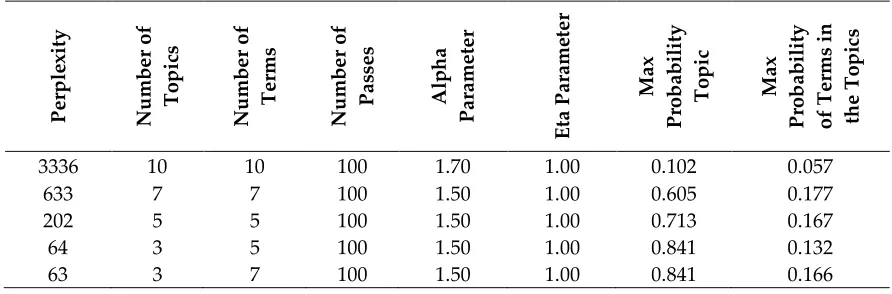
Table 1 demonstrates the pretesting experiments results of preliminary case study of the main
254
parameters of LDA model. The optimum value of the Perplexity index is achieved in the point, when
255
further changes in the parameters do not lead to its significant decrease. In accordance with author’s
256
algorithm, obtained optimal number of latent probabilistic topics will be used as a recommended
257
number of semantic clusters in the LSA-based level of SLR analysis.
258
Table 1. PCS results of the Studying of the of LDA Model Parameters
259
P
er
p
le
xity
Nu
m
b
er
o
f
To
p
ic
s
Nu
m
b
er
o
f
Ter
m
s
Nu
m
b
er
o
f
P
as
ses
A
lp
h
a
P
ar
am
eter
E
ta
P
ar
am
eter
Max
P
ro
b
ab
ility
To
p
ic
Max
P
ro
b
ab
ility
o
f
Ter
m
s
in
th
e
To
p
ic
s
3336 10 10 100 1.70 1.00 0.102 0.057
633 7 7 100 1.50 1.00 0.605 0.177
202 5 5 100 1.50 1.00 0.713 0.167
64 3 5 100 1.50 1.00 0.841 0.132
63 3 7 100 1.50 1.00 0.841 0.166
The list of obtained latent probabilistic topics with information about most probable (significant)
260
terms, described this topic, is presented in the Table 2.
261
Table 2. PCS results of the List of Latent Probabilistic Topics with Distribution of Terms
262
Terms Probability Terms Probability Terms Probability
Topic #0 Topic #1 Topic #2
story 0.080 cinema 0.109 character 0.166
action 0.062 creator 0.066 playing 0.140
effect 0.050 woman 0.062 good 0.130
character 0.047 cast 0.052 character 0.090
book 0.046 stage 0.051 role 0.040
image 0.044 main 0.050 typical 0.030
Step II. LDA-clustering of СF in Semantic Dimensions of Corpus
263
Based on information about the maximum probability of matching the obtained Latent
264
Probabilistic Topics to the CF, on this step the process of Semantic (topical) clustering of CF could be
265
performed. The PCS results of this process are presented in Table 3.
266
Table 3. PCS results of the Semantic Clustering of CF
267
CF CF_5 CF_0 CF_1 CF_4 CF_6 CF_2 CF_3
# topic (cluster) 0 1 1 1 1 2 2
Probability 0.8411 0.6228 0.8022 0.7039 0.4800 0.7957 0.6603
268
The values of the Perplexity in the Table 1 proves the validity of the assumption A2 about
269
providing the analysis the Corpora by paragraphs. But, on the other hand, we can note, that the level
270
of probability of a CF belonging to a particular topic/cluster is not significant for all CF (for example,
271
for CF_6 it is lower than 0.5).
272
3.1.2. The LSA-based Analysis of Latent Semantic Relations Layer
273
LSA-based Analysis of LSR is the layer, which aims to identify the patterns in the relationships
274
between the terms and latent semantic topics. As we already stated, LSA method is based on the
275
principle that terms that are used in the same contexts tend to have similar meanings. For revealing
276
this information about LSR between topics and CF/terms, we need: to assess the degree of semantic
277
correlation relationship between CF/terms via building the reduced model of LSR; to form the
278
semantic clusters of CF via determining the cosine distance between the CF in order to identify the
279
LSR between topics and CF; to form the contextual dictionary of semantic clusters of CF via
280
determining the cosine distances between the terms in order to identify the LSR between k terms and
281
topics.
282
283
Step III. Identifying the Hidden Semantic Connection within the Documents
284
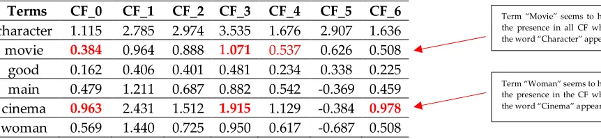
Mathematically the Reduced model, as the instrument of preliminary LSR presence
285
identification, is the process of multiplying of SVD transformation results with chosen k-dimension
286
T K K KKtd U td td V td
X
. The fragment of PCS results of Reduced model is presented in Table 5.
287
Via comparison of the red numbers in Table 5 with zero’s values in the same places of Table 4
288
could be, as an example, identified the existence of the phenomena of LSR:
289
Table 4. The fragment of PCS results of the Absolute Frequency Terms-CF Matrix
290
Terms CF_0 CF_1 CF_2 CF_3 CF_4 CF_5 CF_6 Sum
character 1 1 4 5 2 2 1 16
movie 0 2 1 0 0 1 1 5
good 0 1 0 2 1 3 2 9
main 1 3 0 2 1 0 2 9
cinema 0 3 0 0 1 0 0 4
woman 1 2 1 0 0 0 0 4
291
Table 5. The fragment of PCS results of the Reduced Model for Identifying the LSR
292
Terms CF_0 CF_1 CF_2 CF_3 CF_4 CF_5 CF_6 character 1.115 2.785 2.974 3.535 1.676 2.907 1.636 movie 0.384 0.964 0.888 1.071 0.537 0.626 0.508 good 0.162 0.406 0.401 0.481 0.234 0.338 0.225 main 0.479 1.211 0.687 0.882 0.542 -0.369 0.459 cinema 0.963 2.431 1.512 1.915 1.129 -0.384 0.978
woman 0.569 1.440 0.725 0.950 0.617 -0.687 0.508
Term “Movie” seems to have the presence in all CF where the word “Character” appears
At the same time, we can observe the increasing of the values of the correlation coefficient (CC)
293
between terms, compared the results of Tables 4 and 5 (Table 6):
294
Table 6. Example of PCS results of the Comparison of the CC Between Terms
295
Source Terms
Absolute Frequency Terms-CF Matrix
Reduced Model for Identifying the Hidden Connection
Character. Movie -0.333 0.985
Cinema. Woman 0.641 0.984
Steps IV-VI. Identifying the Degree of Closeness Between the CF / Terms in the Semantic Dimensions of
296
Topics. LSA Clustering of CF / Terms in the Semantic Dimensions of Topics
297
For measuring the level of LSR, identified on the previous step, the matrix of cosine distance
298
between the vectors of СF and terms should be built. Based on the matrices of cosine distances
299
between the vectors of СF and terms, in this step the Semantic clustering process should be realized.
300
An example of the implementation of k-means clustering [18, 30] algorithm for CF and terms (in the
301
condition of LDA-based number of SC) is presented in the Tables 7-8.
302
Table 7. PCS results of the Labels of Contextual Fragments’ Clustering
303
CF CF_0 CF_1 CF_5 CF_2 CF_3 CF_4 CF_6
Cluster 0 0 1 2 2 2 2
3.1.3. Adjustments of the Results of the Two Levels of Analysis
304
On the VII step of Author’s Algorithm, it is supposed to combine the results of the
305
implementation of LSA and LDA levels for analysis, namely:
306
1. Forming the table of the Comparison of the numerical labels of Latent Semantic Clusters of a set
307
of CF, obtained on two levels of research (Table 9). As we can see, the results of clustering for
308
CF_4 and CF_6, obtained in LSA- and LDA-analysis levels, do not match.
309
Table 9. PCS results of the Comparison of the Semantic Clusters as a set of CF Labels
310
LDA-level LSA-level
CF # Topic (Cluster) Probability CF Cluster
CF_0 1 0.6228 CF_0 0
CF_1 1 0.8022 CF_1 0
CF_2 2 0.7957 CF_2 2
CF_3 2 0.6603 CF_3 2
CF_4 1 0.7039 CF_4 2
CF_5 0 0.8411 CF_5 1
CF_6 1 0.4800 CF_6 2
2. Formulation and implementation the Rules of Adjustments of the results obtained in the LSA-
311
and LDA-analysis levels.
312
As stated above, LDA method implementation presupposes the assignment of the
313
corresponding topics to CF based on the largest (from existing) probability (P) of degree of their
314
compliance with the analyzed CF. In this connection, the author’s concept of Rules of Adjustments
315
(RA) of the results of Semantic Clustering of the LSA- and LDA-analysis levels for each particular CF
316
is proposed (Table 10).
317
These rules allow:
318
to improve the quality of LDA-method recognizing the CF’s topics (rules 3, 4) due to the
319
possibility of correcting the results of clustering, which are characterized by the low level of
320
probability of a CF belonging to a particular topic. Suggested instrument – latent semantic
321
specificity of the LSA method;
322
to improve the quality of LSA-method recognition of hidden relations between the CF (rules 2,
323
when CF coordinates located on the cluster’s boundary. Suggested instrument – the probabilistic
325
characteristics of the LDA method.
326
Table 10. Rules of Adjustments of CF Clustering Results
327
Rule LSA-analysis Result
Compari son Result
LDA-analysis Result
LDA Probability
(P)
Assignable Cluster
1 LSA Cluster = LDA Cluster P>0.3 LSA Cluster = LDA Cluster
2 LSA Cluster = LDA Cluster P≤0.3 Cluster is Not recognized
3 LSA Cluster ≠ LDA Cluster P≤0.3 LSA Cluster
4 LSA Cluster ≠ LDA Cluster 0.3<P≤0.7 LSA Cluster /
Re-clustering
5 LSA Cluster ≠ LDA Cluster P>0.7 LDA Cluster
328
The PCS results of the implementation of Rules of Adjustments are presented in Table 11.
329
Table 11. PCS results of the of Final Version of the Labels of the CF’s Semantic Clusters
330
CF CF_5 CF_0 CF_1 CF_4 CF_2 CF_3 CF_6
# topic 0 1 1 1 2 2 2
3.1.4. Case Study Results and Discussion
331
For the process of verification of the author's Methodology in this phase was formed the
332
sentimental structure of FRC via classification of the reviews collection on the Subjectively Positive
333
(SPSC) and Subjectively Negative Sentiment Corpuses (SNSC). This procedure is realized on the basis
334
of information on the subjective evaluations of their tonality (SE) of films by the reviewers (measured
335
by 10-point scale). We consider the SPCS films reviews if the subjective review’s assessment is more
336
than 5 points, and SNCS – if it is equal or less than 5 points.
337
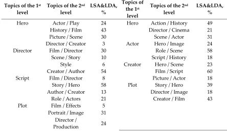
During the verification, the 5000 Polish-language films reviews (2500 SNCS and 2500 SNSC)
338
reviews were analyzed. As a result, two-level Contextual Hierarchical structure of Topics (CHST)
339
was defined (Table 11). The recommended number of clusters (identified in LDA-level of analysis):
340
at the 1st level of hierarchy is equal to 5 for SNCS and is equal to 4 for SNSC;
341
at the 2nd level of hierarchy is equal to 4 for SNCS and is equal to 3 for SNSC.
342
Table 11. PCS results of the of Final Version of the Labels of the CF’s Semantic Clusters
343
Topics of the 1st level
Topics of the 2nd level
LSA&LDA, %
Topics of the 1st
level
Topics of the 2nd level
LSA&LDA, %
Hero Actor / Play 24 Hero Action / History 49
History / Film 43 Director / Cinema 21
Picture / Scene 30 Scene / Actor 31
Director / Creator 3 Actor Hero / Image 24
Director Film / Director 30 Role / Scene 58
Scene / Story 10 Script / History 18
Style 6 Creator Hero / Scene 23
Creator / Author 54 Film / Script 60
Script Film / Director 8 Picture / Actor 18
Story / Hero 58 Plot Story / Hero 39
Author / Creator 13 Director / Image 18
Role / Actors 21 Creator / Film 43
Plot Film / Effects 5
Portrait / Image 31 Director /
344
The Hierarchical structure of the Contextually-Oriented Corpus (HC), created as a two-point
345
(Positive/Negative Classes) structure of the sets of Paragraphs, semantically close to revealed Topics
346
with Contextual Dictionaries (for each separate layer and after adjustment – on the 1st level of Topics)
347
is presented in Table 12 [30, 31]. The Contextual labels (CL) of the Topics were assigned automatically
348
on the bases of the terms with the highest frequency in each topic.
349
Table 12. The Hierarchical structure of the Contextually-Oriented Corpus
350
CL of the 1st level
Topics
SPSC SNSC
LSA,
% LDA, %
LSA&LDA, %
Topics of
the 1st level LSA, % LDA, %
LSA&LDA, %
Hero 29.05 23.50 32.50 Hero 35.10 38.40 37.30
Director 15.80 12.70 10.30 Actor 19.30 20.30 18.30
Script 30.11 26.19 30.94 Creator 28.10 29.10 29.20
Plot 9.50 12.40 15.11 Plot 17.50 12.20 15.20
Spectator 15.54 25.21 11.15
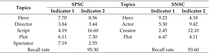
351
The quantitative indicators of the adjustments process of the Latent Semantic Relations Analysis
352
results: percentage of not recognized CF inside the Topic (Indicator 1); percentage of CF, which
353
changed the Cluster (Indicator 2) and as well as final qualitative characteristic of research (Recall rate)
354
the 1st level of Topics are given in Table 13.
355
Table 13. The Quality of the of LSR Analysis Results
356
Topics SPSC Topics SNSC
Indicator 1 Indicator 2 Indicator 1 Indicator 2
Hero 7.70 8.56 Hero 9.23 4.18
Director 3.84 3.44 Actor 5.30 9.42
Script 4.19 16.60 Creator 2.45 12.10
Plot 6.11 7.30 Plot 6.47 4.11
Spectator 7.19 2.55
Recall rate 95.30 Recall rate 93.60
357
In this phase we can conclude that the combination of the Discriminant and Probabilistic
358
Methods (Hypothesis H1) gave the opportunity:
359
to improve the following qualitative characteristics of LSR Analysis: recall rate (as a ratio of the
360
number of semantically clustered/recognized paragraphs to the total number of paragraphs in
361
the corpora) to 90-95%; precision indicator (as the average probability of significantly
362
clustered/recognized paragraphs) from 62 to 70-75%;
363
to increase the depth of recognition of Latent Semantic Relations by providing the a
364
mathematical and methodological basis for building the Contextual Hierarchical structure of
365
Semantic Topics.
366
3.2. Text Classification Based on the Contextually-Oriented Sentiment Dictionary Phase
367
Basic version of Text Classification phaseincludes 9 steps (figure 2).
368
Script / History 40
Spectator Hero / Fan 40
Film / Aspects 20 Role /
Formulation 16
369
Figure 2. The steps of the Text Classification based on the CBSD phase. Source: own research results
370
3.2.1. Creating the Corpora-based Sentiment Dictionary Layer
371
Creating the Corpora-based Sentiment Dictionary is the layer, which aims to identify the
372
Contextually Oriented Hierarchically structured set of Dictionary items (bigrams) and their
373
Sentiment Scores, allowing to measure and evaluate the tonality of the analyzed texts with the high
374
accuracy. One of the two components of bigram must be the elements of Contextual Dictionary of
375
Semantic Clusters (Phase 1). CBSD should have three levels [32]:
376
0s level is the set of Dictionary items without taking into account the Contextual Hierarchical
377
structure of Topics;
378
1st level is the set of Dictionary items with taking into account the 1st level of CHST;
379
2nd level is the set of Dictionary items with taking into account the 2nd level of CHST.
380
To enable the implementation of steps I-IV of the 2nd phase of author’s Methodology (figure 2),
381
only Truly Subjectively Positive (TSP) and Truly Subjectively Negative (TSN) Corpora Samples from
382
Hierarchically structured Contextually-Oriented Corpus (Table 12-13) should be used. To consider
383
the text if the element of TSP, if the subjective text’s assessment is truly positive (more than 8), and
384
the element of TSN – if it is truly negative (assessment less than 4 points) [31].
385
Definition of the Sentiment Scores of the bigrams are estimated by the frequency of occurrence
386
of this bigram in the elements of Corpora. To increase of the degree of accuracy of the Sentiment
387
Scores estimation the parameter to reverse the frequency – RF (Relevance Frequency) is used [33]:
388
) , 1 max( 2 log2
b a
RFS , (9)
where a – number of documents related to category S (positive, negative) and containing this
389
bigram, b – number of documents not related to category S and containing this bigram as well.
390
The purpose of this layer is to evaluate the adequacy and prove the effectiveness of using
391
The main tasks of this layer are:
393
to teach the developed Text Classification algorithm to classify the texts, based on the
394
quantitative measures of the tonality (Sentiment Scores) and with taking into account the one
395
and two-level Hierarchical structure of the Corpora-based Sentiment Dictionary
396
to evaluate the quality of the conducted classification for the purpose of modification /
397
improvement the applied Algorithm via comparing the results of the Text classification.
398
3.2.1. Texts Classification Based on the Manually Created CBSD Layer
399
Steps V-VI. Preparing to Perform the Sentiment Classification Procedure
400
In the step of Training Sample preparing, taking into account the specificity of the case study, as
401
well as limited number of existing software and algorithmic implementations for the analysis of texts
402
in Polish [29], in addition to standard procedures for text pre-processing, the authors have provided
403
text adaptation procedure [30].
404
Step VII. Scanning the Corpora Sample to Identify the Presence of Sentiment Dictionary Elements
405
With the purpose of acceptance / rejection of the Hypothesis 2, this step of algorithm involves
406
the implementation of the following three procedures of scanning the Subjectively Positive/Negative
407
Corpora Samples (SPCS/SNCS).
408
Procedure 1. Using CBSD without taking into account their Topical structure – Simple
409
Classification (step VII.5);
410
Procedure 2. Using CBSD with taking into account their CHST – One-level classification (steps
411
VII.3-5).
412
Procedure 3. Using CBSD with taking into account their CHST – One- and Two-level
413
classification (steps VII.1-5)
414
As was accepted in this study as an Assumption 2, scanning and recognition of topics for One-
415
and Two- Level Classification will be performed by paragraphs (elements of document) [5].
416
For realizing the Procedures 3 (with the deepest Topics Identification process) the following
417
algorithm is developed):
418
Step VII.1. This step realized via scanning the Adopted Training Sample texts and identifying
419
the topics at the 2nd Level of the CHST for each Review paragraph. This procedure is implemented
420
by adding to Training Sample the Topic (Contextual Dictionary elements) from CHST as one of its
421
Paragraphs and then using the LSA method to find paragraphs that have a Latent Semantic
422
Relationships.
423
Step VII.2. This step realized via scanning the part of the Training Sample for which Topics at
424
the 2nd Level were identified, with the aim to find the bigrams form 2nd level of CBSD which
425
correspond to the Topic identified for each Paragraph.
426
Steps VII.3-4. For paragraphs for which topics not been defined in the step VII.1, these steps
427
realized via scanning this part of Adopted Training Sample texts for identifying the topics at the 1st
428
Level of the CHST and subsequent search the bigrams form 1st level of CBSD which correspond to
429
the Topic identified for each Paragraph.
430
Step V. For paragraphs for which topics not been defined in the steps VII.1 and VII 3, these step
431
realized via search the bigrams form 0s level of CBSD.
432
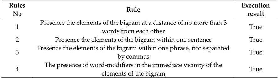
The rules for determining the presence of the elements of the Sentiment Dictionaries and
word-433
modifiers in the text are presented in Table 14.
434
Table 14. Rules for Detecting the Presence of Elements of the Sentiment Dictionary in the Text
436
Rules
No Rule
Execution result
1 Presence the elements of the bigram at a distance of no more than 3
words from each other True
2 Presence the elements of the bigram within one sentence True
3 Presence the elements of the bigram within one phrase, not separated
by commas True
4 The presence of word-modifiers in the immediate vicinity of the
elements of the bigram True
Step IX. Calculation of the Quantitative Measure of the Text Tonality
437
To determine the quantitative measure of the tonality estimate for the entire text of document T
438
from Subjectively Corpora Samples, the number of positive pos C
N , neutral NCneu and negative NCneg
439
bigrams from the corresponding CBSD, found in Texts in accordance with the rules in Table 15, is
440
calculated.
441
Corresponding to the found bigrams Polarity scores
w
ipos,w
ineu andw
ineg are corrected (if442
necessary) taking into account the rules for Words-modifiers and are summed up.
443
pos C
N
i pos i pos
T w
W
1
,
neu C
N
i neu i neu
T w
W
1
,
neg C
N
i neg i neg
T w
W
1
, (10)
where
W
T – weight of text T for particular tonality; wi – Polarity score of bigram i; NC – the444
number of estimated bigrams of particular tonality in the text T.
445
Each texts are placed in a three-dimensional estimated space (positive–neutral–negative tonality)
446
in accordance with their scales
W
T . To find the final basic estimator of the texts tonality we can447
according to the linear function:
448
negT neg neu T pos T neg T neu T pos
T W W W W k W
W
f , ,
, (11)
where kneg is the coefficient, compensating fact of preponderance of positive vocabulary in texts [32].
449
Step IX. Sentiment Text Classification
450
The implementation of this step involves the use of the following rules:
451
Rule 1. Classification for each training sample will be performed in three classes respectively:
452
for Subjectively Positive Corpora Sample (SPCS):
453
C1. Text have the High Positive tonality (HP).
454
C2. Text have the Quite Positive tonality (QP).
455
C3. Text have the Reasonably Positive tonality (RP).
456
for Subjectively Negative Corpora Sample (SNCS):
457
C4. Text have the Rather Negative tonality (RN).
458
C5. Text have the Clearly Negative tonality (CN).
459
C6. Text have the Absolutely Negative tonality (AN).
460
Rule 2. To implement the training procedure for the algorithm being developed, the Sentiment
461
Classifying of texts is suggested using basic quantitative measure of the text tonality [32]:
462
neg
T neu T pos
T
W
W
W
f
Rule 3. Take into account the specificity of chosen case study, to implement the training
463
procedure for the algorithm being developed, the Sentiment Classification is suggested using the
464
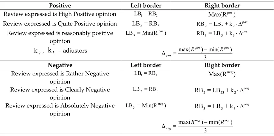
following empirical rules for determining belonging the Text to a certain class (Tables 15-16):
465
466
467
Table 15. Rules for Determining Belonging the Text to a Certain Class (Actual Classes)
468
Positive Left border Right border
Review expressed is High Positive opinion 8 10
Review expressed is Quite Positive opinion 6 7
Review expressed is Reasonably Positive opinion 5
Negative Left border Right border
Review expressed is Rather Negative opinion 3 4
Review expressed is Obviously Negative opinion 2 3
Review expressed is Absolutely Negative opinion 0 1
469
Table 16. Empirical Rules for Determining Belonging the Text to a Certain Class (Predicted Classes)
470
Positive Left border Right border
Review expressed is High Positive opinion LB1=RB2 Max(Rpos)
Review expressed is Quite Positive opinion LB2=RB3
pos
2 2
2 =LB +k
RB
Review expressed is reasonably positive opinion
) Min(R =
LB3 pos
pos
3 3
3=LB +k
RB
2
k
,k
3 – adjustors3
) min( )
max( pos pos pos
R
R
Negative Left border Right border
Review expressed is Rather Negative opinion
2
1=RB
LB Max(Rneg)
Review expressed is Clearly Negative opinion
3 2 =RB
LB neg
2 23 2=LB +k
RB
Review expressed is Absolutely Negative opinion
) Min(R =
LB neg
3
neg
3 3 3 =LB +k
RB
3
) min( )
max( neg neg
neg
R
R
3.2.3. Case Study Results and Discussion
471
For testing and evaluating the adequacy of the Text Classification based on the CBSD phase, as
472
a case study were used the following training samples: for the first layer (CBSD Creation Algorithm)
473
– 5000 Polish-language films reviews (2500 TSP and 2500 TSN); for the second layer (Sentiment
474
Classification Algorithm) – 3000 Polish-language films reviews (1500 SPCS and 1500 SNCS) from the
475
filmweb.pl. To consider the SPCS films reviews, if the subjective review’s assessment is more than 5
476
points, and SNCS – if it is equal or less 5 points.
477
3.2.3.1 CBSD Creation Algorithm
478
As a result of the first layer of the developed methodology the Hierarchical Topically Oriented
479
Corpora-based Sentiment Dictionary was created (Table 17).
480
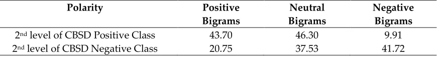
Table 17. The Semantic Structure of CBSD (%)
482
Polarity Positive
Bigrams
Neutral Bigrams
Negative Bigrams
2nd level of CBSD Positive Class 43.70 46.30 9.91
2nd level of CBSD Negative Class 20.75 37.53 41.72
483
The main specificities of the received CBSD [32]:
484
for Positive Class of CBSD: Almost equal numbers of bigrams of neutral and positive polarity.
485
This suggests that half of the adjectives and verbs used to characterize the reviewer's opinion
486
without having a positive coloring, formally confirm (ascertain) the existing facts. 10% of
487
negatively colored bigram, indicating that, despite the truly positive tonality of reviews, the
488
reviewer doubts about the positivity of certain shades (elements) of the film. The greatest
489
number of positively colored Bigram is related to the to the Topics: Role / Actors and Script /
490
History.
491
for Negative Class of CBSD: Almost more bigrams are negative and, are less, neutral polarity.
492
Negative reviews are characterized, in turn, by a large number of oppositely painted bigrams.
493
Perhaps some of these positive emotions are introduced by the authors for comparison or
494
contrast. most of the negatively colored bigram refers to the Topics: Scene / Actor and Role /
495
Scene.
496
3.2.3.2 Sentiment Classification Algorithm
497
Simple Sentiment Classification
498
At the step VII.5 of the developed methodology the algorithm of Sentiment Classification using
499
CBSD 0s level of CBSD (without taking into account their Contextual Hierarchical structure of Topics)
500
was realized (Table 18).
501
Table 18. Evaluation of the Quality of Sentiment Classification of the Films Reviews Results (Simple
502
Classification, in %)
503
SPCS SNCS
C
las
s
%
P
rec
is
io
n
Rec
all
A
cc
u
ra
cy
C
las
s
%
P
rec
is
io
n
Rec
all
A
cc
u
ra
cy
HP 28.57 53.57 51.72
47.96
RN 33.00 33.33 29.73
43.00
QP 47.96 51.06 53.33 CN 56.00 53.57 57.69
RP 23.47 34.78 33.33 AN 11.00 18.18 18.18
504
Additionally, results of comparing the quality of the recognition of the reviews of the films SPCS
505
/ SNCS allowed to draw the following conclusions:
506
1. A large part of reviews is characterized by an average degree of density of the distribution of
507
words with recognizable tonality. This fact complicates the process of an assessment of the rating
508
of the film.
509
2. The morphological analysis of Training Sample testifies that [31]:
510
the positive reviews characterized by highly semantic structured opinion, expressed in a
511
carefully and balanced manner. In this connection, they have a more even (in comparison with
512
negative) distribution of words that have the explicit tonality color.
513
the negative reviews characterized by average level of semantic structure of the opinion,
514
expressed more spontaneously and under the influence of emotions. On the other hand, this
515
spontaneity causes less variability of the words used, and, as a consequence, greater probability
516
of their precise recognition and classification.
517
Realizing the algorithm of Sentiment Classification using the 1st level of CBSD, taking into
519
account the recommendations formulated at the previous stage, allowed:
520
1. Recognize the Sentiment of texts Paragraphs taking into account the 1st level Topics of CBSD
521
(Table 19).
522
Table 19. The Contextual Framework of 1st level of Films Reviews Corpora
523
(% to the total number of paragraphs)
524
Class Hero Director Script Plot Spectator Unrecognized
HP 19.28 57.45 46.38 17.39 45.45
9.29
QP 37.35 34.04 37.68 26.09 31.82
RP 43.37 8.51 15.94 56.52 22.73
Class Hero Actor Creator Plot Unrecognized
RN 57.14 - 44.12 37.84
14.50
CN 28.57 - 47.06 45.95
AN 14.29 - 8.82 16.22
2. Recognize the Sentiment of texts Paragraphs taking into account the 2nd level Topics of CBSD
525
(Table 20).
526
Table 20. The Contextual Framework of 2nd level of Films Reviews Corpora
527
(% to the total number of paragraphs)
528
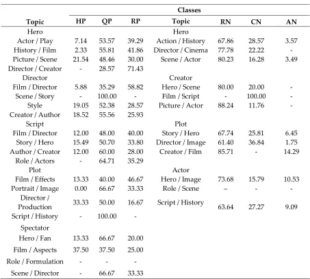
Topic
Classes
HP QP RP Topic RN CN AN
Hero Hero
Actor / Play 7.14 53.57 39.29 Action / History 67.86 28.57 3.57 History / Film 2.33 55.81 41.86 Director / Cinema 77.78 22.22 - Picture / Scene 21.54 48.46 30.00 Scene / Actor 80.23 16.28 3.49 Director / Creator - 28.57 71.43
Director Creator
Film / Director 5.88 35.29 58.82 Hero / Scene 80.00 20.00 -
Scene / Story - 100.00 - Film / Script - 100.00 -
Style 19.05 52.38 28.57 Picture / Actor 88.24 11.76 -
Creator / Author 18.52 55.56 25.93
Script Plot
Film / Director 12.00 48.00 40.00 Story / Hero 67.74 25.81 6.45 Story / Hero 15.49 50.70 33.80 Director / Image 61.40 36.84 1.75 Author / Creator 12.00 60.00 28.00 Creator / Film 85.71 - 14.29
Role / Actors - 64.71 35.29
Plot Actor
Film / Effects 13.33 40.00 46.67 Hero / Image 73.68 15.79 10.53
Portrait / Image 0.00 66.67 33.33 Role / Scene – - -
Director /
Production 33.33 50.00 16.67 Script / History 63.64 27.27 9.09 Script / History - 100.00 -
Spectator
Hero / Fan 13.33 66.67 20.00
Film / Aspects 37.50 37.50 25.00
Role / Formulation - - -
Scene / Director - 66.67 33.33
529
3. To compare the Quality of Simple, One- and Two-level Sentiment Classification of the Films
530
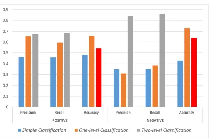
532
Figure 3. The difference between the Average values of Quality evaluation of the One-level and
533
Simple Sentiment Classifying. Source: own research results
534
The general conclusions on the stage of classification can be the following: in comparison with
535
the results of using 0s, 1stand 2nd level of CBSD, the Quality of Sentiment classification has increased
536
significantly.
537
However, a more detailed analysis of the results obtained allows us to identify the following
538
strengths and weaknesses of the conducted stages of text classification:
539
1. Indicators of Precision and Recall for Subjectively Positive Sample grow from 0s Level step to 2nd
540
Level step linearly and gradually. This confirms the previous conclusions that, in general,
541
positive reviews have a higher level of semantic structure and orderliness in expressing
542
emotions. In this regard, the process of recognizing the tonality of the text is better and more
543
accurate even without using the Hierarchical Context Structure of the Sentiment Dictionary;
544
2. Indicators for indicators of Precision and Recall for Subjectively Negative Sample at the 2nd Level
545
step grow steeply. This can be explained by the following facts:
546
during the process of Text Classification using the 1st level of the CBSD, the topic Actor was not
547
recognized for any paragraph of the SNCS. However, when using CBSD of the 2nd level, 2 of 3
548
subtopics of the topic Actor were recognized and assigned to paragraphs of the analyzed sample.
549
This fact, on the one hand, it affected the stepwise increase in the recognition Quality Indicators
550
at the Two-Level Text Classification, on the other hand, it explains the decrease in the Precision
551
Indicator for the One-Level Text Classification;
552
this phenomenon is also explained by the results of research conducted at the previous stages,
553
indicating spontaneous, unstructured and sometimes illogical use of words of different tonality
554
when writing Negative reviews under the influence of emotions.
555
3. A slight decrease in the average Accuracy indicator for the both Samples is could be caused by:
556
too many Topics of the Second level of the Hierarchy used for Reviews analysis
557
provided in the algorithm 6-class Tonality classification of each paragraph,
558
which makes the matrix of the results of the classification sufficiently sparse. For those first level
559
of hierarchy, Accuracy values are much higher.
560
561
562
563
0 0.1 0.2 0.3 0.4 0.5 0.6 0.7 0.8 0.9
Precision Recall Accuracy Precision Recall Accuracy
POSITIVE NEGATIVE