Search | Preprints

(1)

Bayesian VAR Modeling and Forecasting of the Dynamic

Interrelationship between Economic Growth and Revenue from Oil and Non-Oil Sectors in Nigeria+

Monday Osagie Adenomon

Department of Statistics, Nasarawa State University, Keffi, Nasarawa State

Abstract

The present reality about the Nigerian economy calls for investment and development in the non-oil sector. This becomes necessary as a result of fall in the oil price in the global market. This paper examined the Bayesian Vector Autoregression (BVAR) modeling and forecasting of the dynamic interrelationship between Economic growth and revenue from the oil and non-oil sectors in Nigeria. To achieve this, annual data on Gross Domestic Product (GDP), revenue from oil and non-oil sectors were collected from Central Bank of Nigeria (CBN) bulletin, the sample from 1981 to 2008 was used for analysis, while sample from 2009 to 2014 was used for model validation. Six (6) versions of Sims-Zha BVAR models were compared for out-of-sample forecast, the result revealed the superiority of the BVAR6 model over the other BVAR models. Lastly, evidence from the decomposition forecast errors revealed that revenue of oil sector contributed 7.69% to GDP while revenue from non-oil sector contributed 0.12% to GDP in Nigeria. This paper therefore recommended that the present government should encourage investment that is geared toward development in the non-oil sector, of which it has the capacity to improve the Economic growth of the Nigerian economy.

Keywords: Bayesian Vector Autoregression (BVAR), Modeling, Forecasting, Gross Domestic Product (GDP), Economic Growth, Revenue, Oil sector, Non-oil Sector

Introduction

Revenue is defined as all amounts of money received by a government from external sources for example those originating from “outside the government” net of refunds and other correcting transaction, proceeds from issuance debt, sale of investments, agency or private trust transactions, and intra-governmental transfers (Ahmed, 2010; Okwori & Sule, 2016). For instance in Nigeria, provision of economic infrastructures, social services, debt services, providing the Army, the Police, the court system and any other operation of the government, are provided by the Nigerian government through oil revenue, non-oil revenue and federal government independent revenue (Omachi, 2011). Unfortunately, the Nigerian economy has suffers decline in revenue during this period of recession, leading to high inflation rate and leading to shortfalls in government capital and recurrent expenditures.

(2)

The following are related literature review: Ude and Agodi (2012) used cointegration and error correction model to investigate the impact of non-oil revenue on economic growth in Nigeria. They used annual data from 1980 to 2013 and the study revealed that agricultural revenue, manufacturing revenue and interest rate have significant impact on economic growth in Nigeria. Offia (2012) examined the impact of non-oil exports on economic growth in Nigeria from 1986-2010. Results from multiple regression revealed that non-oil export is statistically significant to Nigeria economic growth. In a similar work by Abogan et al (2014) investigated the impact of non-oil export on economic growth in Nigeria between 1980 and 2010. Evidence from ordinary least squares method involving error correction mechanism revealed that the impact of non-oil export on economic growth was moderate. Akwe (2014) investigated the impact of non-oil tax revenue on economic growth in Nigeria. Results from the empirical study revealed a statistical significance of economic growth effects of non-oil tax revenue. Oziengbe (2015) investigated the effects of important penetration and FDI inflows on the performance of Nigera’s non-oil exports in the period from 1981-2012 using the methodology of ARDL (Bounds test) approach to cointegration and error correction analysis. The study indicated that import penetration impacted positively on the performance of Nigeria’s non-oil export in the short run, though its long run impact was negative. The short run and long run impact of FDI on non-oil export performance were not statistically significant. Furthermore, the currency depreciation positively impact the performance of Nigeria’s non-oil export in the long run, but its short run impact was not significant. Okwori & Sule (2016) fitted a long run relationship between GDP and Oil revenue, non-oil revenue, domestic debt and external debt in Nigeria. Evidence from their study revealed that oil revenue, non-oil revenue and external debt are positively related to GDP while domestic debt was negatively related to GDP. Okezie and Azubike (2016) evaluated the contribution of non-oil revenue to government revenue and economic growth in Nigeria from 1980 to 2014. Results from ordinary least squares regression revealed a positive and significant contribution of non-oil revenue to economic growth and positive insignificant contribution to government revenue.

This study therefore examined the contribution of oil and non-oil revenues to Gross Domestic Product (GDP) growth rate in Nigeria using six (6) versions of Sims-Zha Bayesian Vector Autoregressive (BVAR) models for out-of-sample forecast comparison.

Model Specification and Description

Bayesian Vector Autoregression with Sims-Zha Prior

(3)

Sims-Zha BVAR estimates the parameters for the full system in a multivariate regression (Brandt and Freeman, 2006).

Given the reduced form model

1 0 1 0 1 0 1 0 1 0 1 1

and

,

,...

2 ,

1 ,

,

where

.

− − − − − − −



=



=

−

=

+

=

A

u

p

l

A

B

dA

c

u

B

y

B

y

c

y

t t l l t p p t t t



The matrix representation of the reduced form is given as

)

,

0 (

~

,

) 1 ( ) 1 (

+



=

  + + 



X

U

MVN

Y

m T m mp mp T m T



We can then construct a reduced form Bayesian SUR with the Sims-Zha prior as follows. The prior means for the reduced form coefficients are that B1=I and B2, . . . Bp=0. We assume that the prior has a conditional structure that is multivariate Normal-inverse Wishart distribution for the parameters in the model. To estimate the coefficients for the system of the reduced form model with the following estimators

)

,

(

~

and

)

,

(

~

/

is

ts

coefficien

for the

prior

Wishart

inverse

-Normal

the

where

)

ˆ

)

(

ˆ

(

ˆ

)

(

)

(

ˆ

1 1 1 1 1 1

v

S

IW

N

S

X

Y

T

Y

X







+





+



+



−



=





+





+



=

− − − − − −



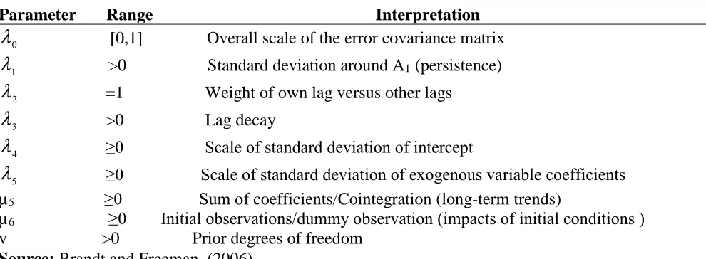
This representation translates the prior proposed by Sims and Zha form from the structural model to the reduced form (Brandt and Freeman, (2006, 2009), and Sims and Zha, (1998, 1999). The summary of the Sims-Zha prior is given in Table 1.0.

Table 1.0: Hyperparameters of Sims-Zha reference prior

Parameter Range Interpretation

0



[0,1] Overall scale of the error covariance matrix

1



>0 Standard deviation around A1 (persistence)

2



=1 Weight of own lag versus other lags

3



>0 Lag decay

4



≥0 Scale of standard deviation of intercept

5



≥0 Scale of standard deviation of exogenous variable coefficients µ5 ≥0 Sum of coefficients/Cointegration (long-term trends)

µ6 ≥0 Initial observations/dummy observation (impacts of initial conditions ) v >0 Prior degrees of freedom

Source: Brandt and Freeman, (2006)

(4)

) 5 0.07, 0.15, 1, 0.15, , 9 . 0 ( BVAR6 2) 0.07, 0.1, 1, 0.1, , 9 . 0 ( BVAR5 2) 0.07, 0.15, 1, 0.15, , 8 . 0 ( BVAR4 2) 0.07, 0.15, 1, 0.15, , 6 . 0 ( BVAR3 5) 0.07, 0.1, 1, 0.1, , 8 . 0 ( BVAR2 5) 0.07, 0.1, 1, 0.1, , 6 . 0 ( BVAR1 6 5 5 4 3 1 0 6 5 5 4 3 1 0 6 5 5 4 3 1 0 6 5 5 4 3 1 0 6 5 5 4 3 1 0 6 5 5 4 3 1 0 = = = = = = = = = = = = = = = = = = = = = = = = = = = = = = = = = = = = = = = = = = = = = = = =                                          

where nµ is prior degrees of freedom given as m+1 where m is the number of variables in the multiple time series data. In this work nµ is 4 (that is three (3) time series variables plus 1(one)). The following are the criteria for Forecast assessments used:

1. Mean Absolute Error (MAE) has a formular 1

n i i j e MAE n =

=



. This criterion measures

deviation from the series in absolute terms, and measures how much the forecast is biased. This measure is one of the most common ones used for analyzing the quality of different forecasts.

2. The Root Mean Square Error (RMSE) is given as

2

(y y )

n f i i j n

RMSE

−



=

_{where y}_i_is

the time series data and yf is the forecast value of y (Caraiani, 2010).

For the two measures above, the smaller the value, the better the fit of the model (Cooray, 2008)

Materials and Methods

The data used in this paper was sourced from CBN 2014 Statistical Bulletin. The data on annual GDP, Oil revenue and non-oil revenue in Nigeria spanned from 1981 to 2014. The unit of measurement for GDP, Oil revenue and non-Oil revenue are all in Billion naira (N). The sample from 1981 to 2008 was used for analysis, while sample from 2009 to 2014 was used for model validation.

Results and Discussion

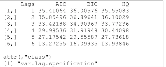
To carry out a BVAR analysis, it is required to obtain the optimal lag for the model. Result from the VAR lag specification revealed lag 6 as the optimal (see table 2 below for detail) Table 2: VAR lag Specification

$ldets

Lags Log-Det Chi^2 p-value [1,] 6 8.090737 44.163130 1.317016e-06 [2,] 5 22.811780 21.768731 9.641553e-03 [3,] 4 26.439902 38.292377 1.544683e-05 [4,] 3 30.694610 39.015096 1.144858e-05 [5,] 2 33.945868 5.607955 7.784235e-01 [6,] 1 34.319732 0.000000 0.000000e+00

(5)

Lags AIC BIC HQ [1,] 1 35.41064 36.00576 35.55083 [2,] 2 35.85496 36.89641 36.10029 [3,] 3 33.42188 34.90967 33.77236 [4,] 4 29.98536 31.91948 30.44098 [5,] 5 27.17542 29.55587 27.73618 [6,] 6 13.27255 16.09935 13.93846

attr(,"class")

[1] "var.lag.specification"

The analysis of the variables (GDP, Oil revenue and non-Oil revenue) using BVAR in R, and the forecast were compared with the actual values of the variable using the forecast assessment criteria and the result is presented in table 3 below.

Table 3: Performance Ratings of the six (6) version of Sims-Zha Bayesian VAR Models RMSE MAE

BVAR1 12532.12 8453.85 BVAR2 12294.701 8360.998 BVAR3 12206.281 8329.391 BVAR4 12020.970 8270.493 BVAR5 12206.281 8329.391

BVAR6 11924.605 8237.353

From the table 3 above the minimum RMSE and MAE is associated with BVAR6. Hence BVAR6 is the best model among others. Details of BVAR6 are presented at the appendix.

Table 4A: Actual Series from 2009 to 2014

Actual Series

Year GDP Oil Revenue Non-Oil Revenue 2009 24794.24 3191.94 1652.65

2010 54612.26 5396.09 1907.58

2011 62980.4 8878.97 2237.88

2012 71713.94 8025.97 2628.78

2013 80092.56 6809.23 2950.56

2014 89043.62 6793.72 3275.12

Table 4B: BVAR6 Forecast Series from 2009 to 2014

Forecast from BVAR6 Model

Year GDP Oil Revenue Non-Oil Revenue 2009 29037.08 8001.757 1612.811

(6)

2012 49022.26 13167.680 2724.771 2013 58297.99 15700.070 3239.744 2014 69353.94 18699.247 3853.369

Model validation used the actual series in Table 4A to compare the forecast from BVAR6 in Table 4B. The Impulse response function for the model is presented at the appendix.

Table 5: Decomposition of Forecast Errors for a Shock to GDP

--- Std. Error gdp oilrev nonoilrev

[1,] 768.5614 84.28936 15.249626 0.4610175 [2,] 1143.1991 88.12734 11.659314 0.2133470 [3,] 1474.9375 90.73917 9.121355 0.1394709 [4,] 1819.1347 92.18394 7.693131 0.1229263

---

In table 5 above on decomposition of forecast errors for a shock to GDP at step 4 revealed that Oil revenue contributed 7.69% to GDP while Non-Oil revenue contributed only 0.12% to GDP in Nigeria. This result revealed that oil revenue still dominates the non-oil revenue in terms of their contribution to GDP in Nigeria which agrees with Omachi (2011) and contradict the findings of Okezie and Azubike (2016). The implication of this finding show some level of overdependence on oil sector and a level of neglect on the non-oil sector.

Conclusion

(7)

References

Abogan, O. P; Akinola, E. B. & Baruwa, O. I.(2014): Non-Oil Export and Economic Growth in Nigeria (1980-2011). JREIF, 3(1):1-11.

Ahmed, Q. M. (2010): Determinants of Tax Buoyancy: Empirical Evidence from Developing Countries. European Journal of Social Sciences, 13(3):408-414.

Akwe, J. A. (2014): Impact of Non-Oil Tax Revenue on Economic Growth: The Nigerian Perspective. Intl Journal of Finance & Accounting, 3(5):303-309.

Brandt, P. T. and Freeman, J. R. (2006): Advances in Bayesian Time Series Modeling and the Study of Politics: Theory, Testing, Forecasting and Policy Analysis. Political Analysis. 14(1):1-36.

Brandt, P. T. and Freeman, J. R. (2009): Modeling Macro-Political Dynamics. Political Analysis. 17(2):113-142.

Caraiani, P. (2010): Forecasting Romanian GDP using A BVAR model. Romanian Journal of Economic Forecasting. 4:76-87.

Cooray, T. M. J. A.(2008): Applied Time series Analysis and Forecasting. New Delhi: Narosa Publising House.

Offia, N. P.(2012): The Impact of Non-Oil Export on Economic Growth in Nigeria (1986-2010). BSc Thesis, Caritas University, Amorji-Nike, Enugu.

Okezie, S. O. & Azubike, J. U.(2016): Evaluation of the Contribution of Non-Oil Revenue to Government Revenue and Economic Growth: Evidence from Nigeria. Journal of

Accounting and Financial Management, 2(5):41-51.

Okwori, J. & Sule, A.(2016): Revenue Sources and Economic Growth in Nigeria: An Appraisal. Journal of Economics and Sustainable Development, 7(8):113-123.

Omachi, A. O.(2011): Effects of Public Revenue on Economic Growth in Nigeria (1980-2008). MSc Thesis, Ahmadu Bello University, Zaria.

Oziengbe, S. A.(2015): Import Penetration, FDI Inflows and Non-Oil Export Performance in Nigeria (1981-2012): A Cointegration and Error Correction Analysis. Botswana Journal of Economics (BOJE), 13(1):40-67.

(8)

Sims, C. A. and Zha, T. (1999): Error Bands for Impulse Responses. Econometrica. 67(5):113-1155.

Ude, D. K. & Agodi, J. E.(2012): Investigation of the Impact of Non-Oil Revenue on Economic Growth in Nigeria. IJSR, 3(11):2571-2577.

Appendix A

--- Sims-Zha Prior reduced form Bayesian VAR --- Prior form : Normal-inverse Wishart Prior hyperparameters :

lambda0 = 0.9 lambda1 = 0.15 lambda3 = 1 lambda4 = 0.15 lambda5 = 0.07 mu5 = 5 mu6 = 5 nu = 4

--- Number of observations : 26

Degrees of freedom per equation : 7 --- Posterior Regression Coefficients :

--- Autoregressive matrices:

B(1)

[,1] [,2] [,3]

[1,] 1.065863 0.053400 0.026101 [2,] 0.234580 0.733754 0.035377 [3,] 0.265913 0.159131 0.710972

B(2)

[,1] [,2] [,3]

[1,] 0.020815 0.031796 -0.004895 [2,] -0.070519 -0.106017 -0.017032 [3,] 0.096299 0.020217 -0.000877

B(3)

[,1] [,2] [,3]

[1,] 0.029628 0.024648 -0.001369 [2,] -0.005843 0.053943 -0.005075 [3,] 0.019319 0.078149 -0.008379

B(4)

[,1] [,2] [,3]

[1,] 0.009202 0.011388 0.001951 [2,] 0.015156 0.067673 0.004021 [3,] 0.049522 0.047226 0.001880

B(5)

[,1] [,2] [,3]

[1,] 0.006134 0.007031 0.000549 [2,] 0.033225 0.033936 -0.003672 [3,] 0.028314 0.006616 -0.006481

B(6)

(9)

[1,] 0.002496 0.000892 -0.000704 [2,] 0.001570 -0.009863 -0.000472 [3,] -0.017998 -0.018567 0.004818

--- Constants

22.09845 -7.788908 0.06743

--- --- Posterior error covariance

[,1] [,2] [,3]

[1,] 497885.96 211774.23 -36821.56 [2,] 211774.23 254821.12 -11341.83 [3,] -36821.56 -11341.83 29473.70

---

Appendix B

1 3 5

-5 e + 0 9 -1 e + 0 9 gdp gdp

1 3 5

-3 .0 e + 0 9 0 .0 e + 0 0 o ilr e v

1 3 5

0 e + 0 0 6 e + 0 8 n o n o ilr e v

1 3 5

-5 e + 0 9 -1 e + 0 9 oilrev

1 3 5

-3 .0 e + 0 9 0 .0 e + 0 0

1 3 5

0 e + 0 0 6 e + 0 8

1 3 5

-5 e + 0 9 -1 e + 0 9 nonoilrev

1 3 5

-3 .0 e + 0 9 0 .0 e + 0 0

1 3 5

0 e + 0 0 6 e + 0 8 R e sp o n se i n Shock to

Appendix C

Decomposition of Forecast Errors for a Shock to gdp

--- Std. Error gdp oilrev nonoilrev

(10)

[2,] 1143.1991 88.12734 11.659314 0.2133470 [3,] 1474.9375 90.73917 9.121355 0.1394709 [4,] 1819.1347 92.18394 7.693131 0.1229263

--- Decomposition of Forecast Errors for a Shock to oilrev --- Std. Error gdp oilrev nonoilrev

[1,] 406.0257 0.000000 99.93128 0.06871849 [2,] 514.4502 3.632023 96.14352 0.22445996 [3,] 568.3475 10.222174 89.44650 0.33132222 [4,] 617.2525 18.473032 81.15791 0.36905860

--- Decomposition of Forecast Errors for a Shock to nonoilrev --- Std. Error gdp oilrev nonoilrev

[1,] 163.2092 0.000000 0.000000 100.00000 [2,] 206.5427 4.415172 1.581163 94.00367 [3,] 247.8532 18.995612 4.127369 76.87702 [4,] 303.8179 37.475378 7.197465 55.32716