Adaptively Secure, Universally Composable, Multi-Party Computation in Constant Rounds

(1)

Adaptively Secure, Universally Composable,

Multi-Party Computation in Constant Rounds

Dana Dachman-Soled∗ Jonathan Katz∗† Vanishree Rao‡

Abstract

Cryptographic protocols withadaptive security ensure that security holds against an adver-sary who can dynamically determine which parties to corrupt as the protocol progresses—or even after the protocol is ﬁnished. In the setting where all parties may potentially be cor-rupted, and secure erasure is not assumed, it has been a long-standing open question to design secure-computation protocols with adaptive security running inconstant rounds.

Here, we show a constant-round, universally composable protocol for computing any func-tionality, tolerating a malicious, adaptive adversary corrupting any number of parties. Interest-ingly, our protocol can computeall functionalities, not just adaptively well-formed ones.

1 Introduction

When designing and analyzing protocols for secure computation, there are several diﬀerent ad-versarial models one can consider. The original deﬁnitions of security assume a static adversary who decides which parties to corrupt before execution of the protocol begins. Subsequently [3, 9], researchers began to consider the more challenging setting in which the adversary may adaptively decide which parties to corrupt as the protocol progresses—or even after the protocol ends. It is easy to come up with examples of protocols that are secure in a static-corruption model, but that are trivially insecure in the adaptive setting.

Even in a setting where adaptive corruptions are considered, there are different assumptions one can make. Initial work on adaptive security [3] made the assumption that honest parties can securely erase local data (e.g., randomness or other internal state) when no longer needed. Later work, led by Canetti et al. [9], sought to avoid this assumption, arguing that it is unwise to rely on other parties to erase data (since there is no way such erasure can be verified) and that it is generally difficult—even for an honest party who intends to erase data—to ensure that all traces of data are gone. Whether or not erasure is assumed has a significant impact on the complexity of adaptively secure protocols; for example, adaptively secure public-key encryption is fairly simple and efficient [3] if erasure is assumed, but much more complicated (and much less efficient) [9, 2, 15, 13] without this assumption. Similarly, adaptively secure two-party computation is much easier with the assumption of secure erasure [26] than without [11].

Designing protocols without the assumption of secure erasure is diﬃcult, in part, due to the need to deal with post-execution corruption (PEC), whereby an adversary can corrupt parties

∗_{University of Maryland. Email:} _{[email protected],}_{[email protected].} †_{Work supported in part by NSF awards #1111599 and #1223623.}

(2)

(and hence obtain the randomness they used) even after execution of the protocol has concluded. Handling PEC is inherent to the setting of universal composability (UC) [7], and is important for ensuring sequential composition even in the stand-alone setting [6]. If secure erasure is assumed, the deﬁnition of adaptive security does not change whether or not PEC is allowed [8], but without erasure the requirement of dealing with PEC adds signiﬁcant additional complications.

Prior work. We are interested in adaptive security, with PEC, in a model where secure erasure is not assumed. Some prior protocols for secure computation in this setting (e.g., [9, 2]) assume a majority of the parties remain uncorrupted. Other work [24, 23, 18, 21], including concurrent work of [16], allowsall but one of the parties to be corrupted. While it may seem strange to worry about corruption ofall parties, consideration of this case is important when a protocol Πouter invokes some

protocol Πinner (not involving all parties running Πouter) as a subroutine. In this case, all parties

running Πinner may eventually be corrupted, and security of Πouter should still be guaranteed.

To the best of our knowledge, all prior work giving adaptively secure protocols for general functionalities (without erasure), and tolerating an arbitrary number of corruptions, are based on the Goldreich-Micali-Wigderson [19] paradigm for semi-honest computation, and thus have round complexity linear in the depth of the circuit being computed. These include protocols in the common reference string model [11], the “sunspots” model [12], the key-registration model [1], and, more generally, based on adaptively secure UC puzzles [14]. In addition, all prior work in this setting handles only “adaptively well-formed functionalities” (see [11] for a deﬁnition).

1.1 Our Result

We show a constant-round, universally composable protocol for multi-party computation of arbi-trary functionalities, with security against a malicious, adaptive adversary corrupting any number of parties. Once again, we stress that we do not assume secure erasure.

Overview of our techniques. The main diﬃculty in our setting is to construct a constant-round protocol with security against asemi-honest, adaptive adversary corrupting any number of parties. Given any such protocol, we can compile it as in [11] to obtain a universally composable protocol with security against a malicious, adaptive adversary, and still running in constant rounds. We may also assume secure channels, which can be implemented using adaptively secure encryption.

Our protocol in the semi-honest setting relies on a common reference string (CRS). While it would be more elegant to avoid this assumption, note that a CRS—or some other form of setup— is anyway needed [10] in order to obtain universally composable computation in the presence of malicious adversaries corrupting half or more of the parties, even in a static-corruption model. Thus, as far as our ﬁnal result (i.e., our protocol with security in the malicious setting) is concerned, some form of setup is unavoidable. We remark further that results of Garg and Sahai [18] indicate that a CRS (or some other form of setup) is needed to obtain constant-round protocols with adaptive security even in the semi-honest case; see further discussion at the end of this section.

(3)

and then outputting (output,Explain(input,output)). That is, the Explain algorithm provides the ability to sample random coins for Algf that “explain” any given input/output pair.

Sahai and Waters [27] introduced the notion of explainability for the speciﬁc case of public-key encryption schemes, in the context of constructing a deniable encryption scheme. We observe that their techniques can be suitably generalized to give an explainable version of arbitrary algorithms based on indistinguishability obfuscation for general circuits (and one-way functions). We refer the reader to Section 3 for a formal statement of this result.

Let C be a circuit taking n-bit inputs.1 Consider the following functionality NextMsg that (essentially) computes the next-message function for a two-round secure-computation protocol for C based on garbled circuits: NextMsg takes as input a sequence of ﬁrst-round messages

OT1,1, . . . ,OT1,n for a two-round, adaptively secure, oblivious-transfer (OT) protocol (e.g., the protocol of [11]); it then (1) computes a garbled circuit GC corresponding toC, along with input-wire labels{(yi,0, yi,1)}ni=1, and (2) computes a sequence of OT responsesOT2,1, . . . ,OT2,n. (These responses allow the party that generatedOT1,iusing input bitbto recoveryi,b while learning noth-ing aboutyi,1−b.) The output ofNextMsg is (GC,OT2,1, . . . ,OT2,n). The CRS for our protocol will beNextMsg^ , an explainable version ofNextMsg.2 _{We note that, in contrast to [27], in the real-world} execution no parties have access to the Explainalgorithm corresponding to NextMsg^ .

Our multi-party protocol computing C can now be described quite simply. The protocol pro-ceeds in four rounds. Say we have n parties P1, . . . , Pn holding inputs x1, . . . , xn, respectively. These parties generate ﬁrst-round OT messages OT1,1, . . . ,OT1,n (with the party who is sup-posed to provide the ith input generating OT1,i), and send these to Pn. Party Pn then runs

^

NextMsg(OT1,1, . . . ,OT1,n) to obtain GC,OT2,1, . . . ,OT2,n, and sends OT2,i to the corresponding party (which might be itself). Each party Pi then locally recovers yi, the label for the ith input wire of the garbled circuit, and sends yi toPn. Finally, Pn evaluates the garbled circuit GC using the provided input-wire labels to obtain the outputz, and sendsz to all the other parties.3 Only the third- and fourth-round messages need to be sent via a secure channel.

We now describe the simulator informally. Our simulator begins by generating NextMsg^ along with its associatedExplainalgorithm, and lettingNextMsg^ be the CRS. It simulatesOT1,1, . . . ,OT1,n andOT2,1, . . . ,OT2,n using the simulator for the OT protocol (recall the OT protocol is adaptively secure), and uses these for the ﬁrst two rounds of the protocol. Upon corruption of party Pi, the simulator corrupts that party in the ideal world and learns its inputxi and the output z. Then:

• If this is the ﬁrst corruption, the simulator generates a simulated garbled circuitGCconsistent with output z, along with n input-wire labels y1, . . . , yn. It also uses the Explain algorithm to generate random coinsr∗ consistent with runningNextMsg^ on inputOT1,1, . . . ,OT1,n and obtaining outputGC,OT2,1, . . . ,OT2,n.

• The simulator uses the simulator for the OT protocol to generate internal state forPi consis-tent with input xi and outputyi, and returns this to the adversary. In addition, if P =Pn then it returnsr∗ to the adversary.

1

We assume for simplicity here thatCis deterministic. Randomized functionalities are handled in Section 4. 2_{As described, the CRS depends on the circuit}_C_{. However, by taking}_C _{to be a universal circuit, the CRS can} be ﬁxed independently of the “actual” function the parties wish to compute.

(4)

Impossibility results? We brieﬂy mention two impossibility results regarding (constant-round) adaptively secure computation, and explain why they do not apply in our setting.

First, our protocol can compute arbitrary randomized functionalities, not just adaptively well-formed ones. (We refer to [11] for a deﬁnition of this term.) This may seem somewhat surprising in light of an impossibility result of Ishai et al. [22] showing that adaptively secure computation of all functionalities (and not just well-formed ones) is impossible. A closer examination of their result, however, reveals that it does not hold in the CRS model.4

Second, Garg and Sahai [18] show that no constant-round, adaptively secure, multi-party pro-tocol can be proven secure using black-box techniques; although they only claim this result for protocols with security against malicious adversaries, their proof appears to extend to the case of semi-honest adversaries as well. Their impossibility result, though, explicitly only applies to the “plain” model where no setup is assumed, whereas in our work we assume a CRS.

1.2 Organization of the Paper

We review some standard cryptographic background and primitives in Section 2. In Section 3, we introduce the notion of anexplainable algorithm, and show how the Sahai-Waters compiler [27] can be used to make any algorithm explainable. Finally, in Section 4 we present a constant-round multi-party computation protocol tolerating a semi-honest, adaptive adversary corrupting any number of parties. Applying the compiler of Canetti et al. [11] yields a constant-round protocol tolerating a malicious, adaptive adversary corrupting any number of parties.

2 Preliminaries

We letλdenote the security parameter. We refer to previous work [6, 8, 26] for deﬁnitions of secure computation in the adaptive-corruption setting (with PEC).

2.1 Garbled Circuits

We rely on the standard notion of garbled circuits [28]. However, we use slightly non-standard notation that we introduce here. LetCbe a randomized circuit takingn-bit inputs and usingλbits of randomness. We abstract the construction/evaluation of a garbled circuit for C via algorithms

GenGC,EvalGCwith the following properties. GenGCis a randomized algorithm that takes as input 1λ andC, and outputs a garbled circuitGCalong with 2ninput-wire labelsy1,0, y1,1, . . . , yn,0, yn,1 ∈ {0,1}λ and 2λ random-wire labels w1,0, w1,1, . . . , wλ,0, wλ,1 ∈ {0,1}λ. Deterministic algorithm

EvalGC takes as input GCand n+λlabelsy1, . . . , yn, w1, . . . , wλ, and outputs a value z. Correctness requires that for any GC, ({yi,0, yi,1}ni=1,{wi,0, wi,1}λi=1

)

output by GenGC(1λ, C), any x∈ {0,1}n and any r∈ {0,1}λ, we have

EvalGC

(

GC,{yi,xi}

n

i=1,{wi,ri}

λ i=1

)

=C(x;r).

Security requires an eﬃcient simulator SimGC such that for allx, r, the distribution

{(

GC,{(yi,0, yi,1)}ni=1,{(wi,0, wi,1)}λi=1

)

←GenGC(1λ, C) :

(

GC,{yi,xi}

n

i=1,{wi,ri}

λ i=1

)}

is computationally indistinguishable from the output of SimGC(1λ_{, C, C}₍_x_;_r_)).

(5)

2.2 Adaptively Secure Oblivious Transfer

Our protocol uses a two-round, semi-honest, adaptively secure OT protocol as a building block. A suitable construction can be found in [11].

A two-round OT protocol ΠOT comprises three algorithms: a receiver algorithmROT, a sender

algorithmSOT, and an evaluation algorithmEOT. AlgorithmROTtakes as input a bitband random

coinsrR, and outputs initial message OT1. AlgorithmSOT takes as input an initial messageOT1, a pair of λ-bit strings (y0, y1), and randomness rS, and outputs message OT2. The evaluation algorithm EOT takes as input b, rR, andOT2 and outputs theλ-bit stringyb.

For our purposes we require the following property that is implied by semi-honest, adaptive security of ΠOT. There is exist an eﬃcient simulator SimOT = (SimOT1,SimOT2), where SimOT2 is deterministic, such that (1) SimOT1 outputs a transcript (OT1,OT2) along with state st and (2)SimOT2, given as inputb, y, andst, outputs coinsrRfor the receiver consistent with (OT1,OT2) and the receiver holding input band obtaining output y; for anyb, y0, y1, the distribution

{

rR, rS ← {0,1}∗;OT1 :=ROT(b;rR) :

(

rR,OT1, SOT(OT1, y0, y1;rS)

)}

is computationally indistinguishable from

{

(OT1,OT2,st)←SimOT1(1λ);

rR:=SimOT2(1λ, b, yb,st)

: (rR,OT1,OT2)

}

.

That is, we only require “one-sided security” [21] for adaptive corruption of the receiver.

If we deﬁne algorithm SimOT′₁(1λ) to run SimOT1(1λ) and output only (OT1,st), and deﬁne the algorithm SimOT′₂(1λ, b,st) to simply run SimOT2(1λ, b,0λ,st), then for anyb the distribution

{

rR← {0,1}∗:

(

rR, ROT(b;rR)

)}

is computationally indistinguishable from

{

(OT1,st)←SimOT′1(1λ);

rR:=SimOT′2(1λ, b,st)

: (rR,OT1)

}

.

2.3 Indistinguishability Obfuscation

We use an indistinguishability obfuscator as a building block. A ppt machine iO is an indistin-guishability obfuscator for a circuit class{Cλ} if the following conditions are satisﬁed:

Correctness. For allλ, and allC ∈ Cλ, it holds thatC andiO(1λ, C) compute the same function.

Polynomial slowdown. There is a polynomialp(·) such that|iO(1λ, C)| ≤p(λ)·|C|for allC∈ Cλ.

Indistinguishability. For any sequence{(Cλ,0, Cλ,1,auxλ)}λ where Cλ,0, Cλ,1 ∈ Cλ, Cλ,0 ≡ Cλ,1, and|Cλ,0|=|Cλ,1|, and anypptdistinguisherD, there is a negligible functionneglsuch that:

Pr[D(iO(1λ, Cλ,0),auxλ) = 1]−Pr[D(iO(1λ, Cλ,1),auxλ) = 1]≤negl(λ).

When clear from the context, we will often omit the security parameter 1λ as an input toiO and as a subscript forC.

(6)

3 Explainability Compilers

Sahai and Waters [27] deﬁne a notion of explainability for public-key encryption, and show a compiler that transforms any public-key encryption scheme into an explainable version. Here, we generalize the notion of explainability for an arbitrary algorithm Alg, and show that the Sahai-Waters compiler can be used to transform any algorithmAlg into an explainable versionAlgf.

At a high level, an explainability compiler takes as input (a description of) a randomized algo-rithm Alg, and outputs two algorithms Algf,Explain. The ﬁrst of these is a randomized algorithm computing the same functionality as Alg. The second algorithm, roughly speaking, takes an in-put/output pairinput,outputand produces random coins r consistent with runningAlgf(input) and obtaining the resultoutput. That is, the algorithm “explains” the input/output pair input,output. We now give a formal deﬁnition.

Definition 1. A pptalgorithmCompis an explainability compilerif for every eﬃcient, randomized circuit Alg, the following hold:

Polynomial slowdown. There is a polynomial p(·) such that, for any (Algf,Explain) output by

Comp(1λ_,_Alg₎ _{it holds that} _|_Algf_{| ≤}_p₍_λ₎_{· |}_Alg_|_.

Statistical functional equivalence. With overwhelming probability over choice of (Algf, ⋆) as output by Comp(1λ,Alg) the distribution of Algf(input) is statistically close to the distribu-tion of Alg(input) for all input.

Explainability. The success probability of every non-uniform, polynomial-time adversaryAin the following experiment is negligibly close to 1/2:

1. A(1λ₎ _outputs _input∗ _{of its choice.}

2. Comp(1λ,Alg) is run to obtain (Algf,Explain).

3. Choose uniform coins r0∈ {0,1}∗ and compute output∗ :=Algf(input∗;r0).

4. Compute r1←Explain(input∗,output∗).

5. Choose a uniform bit band give Algf,output∗, rb to A. 6. A outputs a bit b′, andsucceeds if b′ =b.

We highlight one key difference between our definition and the corresponding one from [27]: in our case input∗ is an arbitrary length value (depending on the domain of Alg) chosen by the adversary, whereas in [27] the input to the explainable algorithm is a single bit chosen uniformly (and given to the adversary). Because of this, and due to the way the explainability compiler is constructed, we require the adversary to chooseinput∗“non-adaptively,” i.e., before being givenAlgf. This definition of explainability suffices for our eventual protocol.

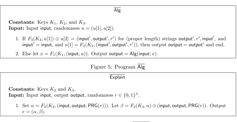
3.1 Constructing an Explainability Compiler

(7)

Alg

Hardwired constants: KeysK1,K2, andK3. Input: Inputinputand randomnessu= (u[1], u[2]).

1. Letinput′,output′, r′) := F3(K3, u[1])⊕u[2]. If it is the case thatinput =input′ andu[1] = F2(K2,(input′,output′, r′)), then outputoutput:=output′ and end.

2. Else letx:=F1(K1,(input, u)) and outputoutput:=Alg(input;x) and end.

Figure 1: ProgramAlg

• Apuncturable, extracting PRFF1(K1,·) that accepts inputs of lengthℓ1+ℓ2+ℓin, and outputs strings of length ℓr. It is extracting when the input min-entropy is greater than ℓr+ 2λ+ 4, with statistical closeness less than 2−(λ+1)_{. Observe that} _ℓ

in+ℓ1+ℓ2≥ℓr+ 2λ+ 4, and thus if one-way functions exist then such a PRF exists by Theorem 4.

• Apuncturable, statistically injectivePRFF2(K2,·) that accepts inputs of length 2λ+ℓin+ℓout,

and outputs strings of lengthℓ1. Observe thatℓ1≥2·(2λ+ℓin+ℓout) +λ, and thus if one-way

functions exist then such a PRF exists by Theorem 3.

• ApuncturablePRFF3(K3,·) that accepts inputs of lengthℓ1and outputs strings of lengthℓ2. If one-way functions exist, then such a PRF exists by Theorem 2.

We deﬁne Comp(1λ,Alg) as follows. Let Alg : {0,1}ℓin × {₀_,₁}ℓr → {₀_,₁}ℓout _{be an algorithm} with domain {0,1}ℓin_{, range} {₀_,₁}ℓout_{, and randomness length} _ℓ

r. Our compiled program Algf will take input input ∈ {0,1}ℓin _{and randomness} _u _{= (}_u_[1]_{, u}_{[2]) of length} _ℓ

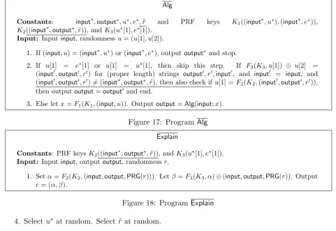
1 +ℓ2, where |u[1]|= ℓ1 = 5λ+ 2(ℓin+ℓout) +ℓr and |u[2]| =ℓ2 = 2λ+ℓin+ℓout. Our compiler ﬁrst samples keys K1,K2, and K3 for PRFs F1, F2, and F3, respectively. It then deﬁnes algorithms Alg and Explain as in Figures 1 and 2, respectively. Finally, it computes Algf ←iO(Alg) and Explain←iO(Explain), and outputs (Algf,Explain).

The proofs of security for our compiler, given for completeness in Appendix B, follow closely along the lines of the analogous proofs in [27]. Speciﬁcally, the proof of statistical functional equivalence closely follows the proof used by Sahai and Waters to establish IND-CPA security of their deniable encryption scheme, and the proof of explainability follows the Sahai-Waters proof establishing explainability of their deniable encryption scheme. We highlight, however, that in our proof of explainability a diﬀerence arises because in our case the inputinput∗ is an arbitrary length value (depending on the domain of Alg), whereas in [27] the input is just a single bit. We are able to adapt the proof to this case because we do not allow input∗ to depend on Algf.

Explain

Hardwired constants: KeysK2 andK3. Input: input,output, and randomnessr∈ {0,1}λ.

1. Setα:=F2(K2,(input,output,PRG(r))) and letβ:=F3(K3, α)⊕(input,output,PRG(r)). Output (α, β).

(8)

NextMsg

Inputs: OT1,1, . . . ,OT1,n; randomnessr1, . . . , rλ∈ {0,1} andrGC, rS,1, . . . , rS,n∈ {0,1}∗.

1. Run GenGC(1λ_{, C}_;_r

GC) to produce the garbled circuit GC along with n pairs of input-wire

labels{(yi,0, yi,1)}ni=1 andλpairs of random-wire labels{(wi,0, wi,1)}λi=1.

2. Fori∈[n], runSOTon inputOT1,iand (yi,0, yi,1) using randomnessrS,i, to obtainOT2,i.

3. OutputGC, OT messages{OT2,i}in=1, and random-wire labelsw1,r1, . . . , wλ,rλ.

Figure 3: Algorithm NextMsg. The security parameter 1λ and circuitC are hardwired.

4 A Semi-Honest, Adaptively Secure Protocol

We describe here a protocol for secure computation of a randomized circuit C by a set of parties

P1, . . . , Pn. We assume for simplicity that all parties learn the output of C; using standard tech-niques, we can handle the general case in which each party learns a possibly diﬀerent function of the inputs. For ease of notation, we assume that the domain ofC is{0,1}nwith partyPi providing theith inputxi∈ {0,1}. (One can easily verify that our protocol and proof generalize to the case of arbitrary-length inputs.) We also assume without loss of generality thatC usesλrandom bits.

The CRS of our protocol is an “explainable” versionNextMsg^ of the algorithmNextMsgdeﬁned in Figure 3. That is, the CRS is generated by computing (NextMsg^ ,Explain)←Comp(1λ,NextMsg) and letting the CRS be NextMsg^ . As described, the CRS depends on C (since NextMsg does); however, by letting C be a universal circuit the CRS can be ﬁxed independently of the “actual” function the parties wish to compute. We note that we allow the environment Z to choose the parties’ inputs depending on the CRS.

Let ΠOT = (ROT, SOT, EOT) be a two-round, semi-honest, adaptively secure OT protocol (cf.

Section 2.2). Our secure-computation protocol Π is deﬁned in Figure 4. We describe the protocol assuming the existence of secure channels; these can be instantiated using any adaptively secure public-key encryption scheme.

Theorem 1. Assume Comp is an explainability compiler, and GenGC and ΠOT satisfy the deﬁni-tions from Secdeﬁni-tions 2.1 and 2.2, respectively. Then protocol Π in Figure 4 UC-realizes functional-ity C in the presence of a semi-honest, adaptive adversary corrupting any number of parties.

Proof: Let SimGC, SimOT denote appropriate simulators as defined in Section 2. Fix an envi-ronmentZ and a dummy adversaryAattacking protocol Π. Recall that we allow the environment Z to adaptively choose the inputs of all partiesafter seeing the common reference string. Without loss of generality, we assume Z first observes the entire protocol transcript (which, since we use secure channels in rounds 3 and 4, consists only of the messages sent in the first two rounds) before corrupting any parties. Our simulatorSim for this adversary proceeds as follows:

1. Compute (NextMsg^ ,Explain)←Comp(1λ,NextMsg), and give NextMsg^ toZ as the CRS. 2. RunSimOT1(1λ) a total ofntimes to obtain{(OT1,i,OT2,i,sti)}ni=1. GiveOT1,1, . . . ,OT1,n−1

toZ as the ﬁrst-round message, andOT2,1, . . . ,OT2,n−1 toZ as the second-round message. 3. When Z requests to corrupt partyPi, corruptPi in the ideal world to learn its input xi and

(9)

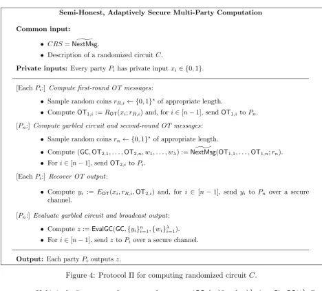
Semi-Honest, Adaptively Secure Multi-Party Computation

Common input:

• CRS =NextMsg^ .

• Description of a randomized circuit C.

Private inputs: Every partyPi has private inputxi∈ {0,1}.

[EachPi:] Compute ﬁrst-round OT messages:

• Sample random coinsrR,i← {0,1}∗ of appropriate length.

• ComputeOT1,i:=ROT(xi;rR,i) and, fori∈[n−1], sendOT1,ito Pn.

[Pn:] Compute garbled circuit and second-round OT messages:

• Sample random coinsrn← {0,1}∗of appropriate length.

• Compute (GC,OT2,1, . . . ,OT2,n, w1, . . . , wλ) :=NextMsg^ (OT1,1, . . . ,OT1,n;rn). • Fori∈[n−1], sendOT2,i toPi.

[EachPi:] Recover OT output:

• Compute yi := EOT(xi, rR,i,OT2,i) and, for i ∈ [n−1], send yi to Pn over a secure

channel.

[Pn:] Evaluate garbled circuit and broadcast output:

• Computez:=EvalGC(GC,{yi}n

i=1,{wi}λi=1).

• Fori∈[n−1], sendzto Pi over a secure channel.

Output: Each partyPi outputsz.

Figure 4: Protocol Π for computing randomized circuit C.

• If this is the ﬁrst party to be corrupted, compute (GC,{yi}n_i₌₁,{wi}λ_i₌₁)←SimGC(1λ, C, z) and rn ← Explain((OT1,1, . . . ,OT1,n),(GC,OT2,1, . . . ,OT2,n, w1, . . . , wn)). Store these values to be used, as needed, in the rest of the simulation.

• In any case, compute rR,i := SimOT2(1λ, xi, yi,sti) and give xi, z, yi, and rR,i toZ. In addition, ifi=n give{yi}in=1−1 and rn∗ toZ.

4. Output whateverZ outputs.

We prove that the output ofZ when interacting withAand parties in a real-world execution of protocol Π is indistinguishable from the output ofZwhen interacting withSimand the functionality

C in an ideal-world execution of the protocol. We do so by considering a sequence of hybrid experiments, beginning with the real-world execution and ending with the ideal-world execution, and showing that each experiment is computationally indistinguishable from the preceding one.

(10)

1. Compute (NextMsg^ ,Explain) ← Comp(1λ,NextMsg), and give NextMsg^ to Z as the CRS. Z chooses inputsx1, . . . , xn.

2. Fori∈[n], sample coinsrR,i and computeOT1,i:=ROT(xi;rR,i). Give the sequence of values

OT1,1, . . . ,OT1,n−1 toZ as the ﬁrst-round message. 3. Sample coinsrnand compute

(GC,OT2,1, . . . ,OT2,n, w1, . . . , wλ) :=NextMsg^ (OT1,1, . . . ,OT1,n;rn).

GiveOT2,1, . . . ,OT2,n−1 toZ as the second-round message.

4. When Z requests to corrupt party Pi, compute yi := EOT(xi, rR,i,OT2,i) and give xi, z, yi, andrR,i toZ. In addition, ifi=nthen computeyi :=EOT(xi, rR,i,OT2,i) fori∈[n−1] and give {yi}ni=1−1 and rn toZ.

Hybrid 1. This experiment is similar to the previous one, except that theOT1 messages and the random coins{rR,i}are generated by the simulator for the OT protocol (cf. Section 2.2). That is, the experiment proceeds via the following steps:

2. Run SimOT′₁(1λ) a total of n times to obtain {(OT1,i,sti)}ni=1. Give the sequence of values

OT1,1, . . . ,OT1,n−1 toZ as the ﬁrst-round message. 3. Sample coinsrnand compute

4. WhenZ corrupts partyPi, computerR,i :=SimOT′2(1λ, xi,sti) andyi:=EOT(xi, rR,i,OT2,i), and give xi, z, yi, and rR,i to Z. In addition, if i = n then for i ∈ [n−1] compute rR,i :=

SimOT′₂(1λ, xi,sti) and yi:=EOT(xi, rR,i,OT2,i), and give {yi}in=1−1 andrn toZ.

It follows immediately by security of the OT protocol (and a straightforward hybrid argument) that this experiment is computationally indistinguishable from the previous one.

Hybrid 2. This experiment is similar to the previous one, except that we now use the Explain

algorithm to generate the random coinsrn. That is, the experiment proceeds as follow:

2. Run SimOT′₁(1λ) a total of n times to obtain {(OT1,i,sti)}ni=1. Give the sequence of values

(11)

3. Sample coinsrnand compute

In addition, letinput∗ = (OT1,1, . . . ,OT1,n) andoutput∗= (GC,OT2,1, . . . ,OT2,n, w1, . . . , wλ), and computer∗ ←Explain(input∗,output∗).

4. WhenZ corrupts partyPi, computerR,i :=SimOT′2(1λ, xi,sti) andyi:=EOT(xi, rR,i,OT2,i), and give xi, z, yi, and rR,i to Z. In addition, if i = n then for i ∈ [n−1] compute rR,i :=

SimOT′₂(1λ, xi,sti) and yi:=EOT(xi, rR,i,OT2,i), and give {yi}ni=1−1 andr∗n toZ.

Computationally indistinguishability of this experiment from the previous one follows from the definition of explainability (cf. Definition 1), and the fact that Compis an explainability compiler. To see this, say there is an efficient adversaryZand a non-uniform, polynomial-time distinguisherD

that distinguishes the outcome of Hybrid 1 from that of Hybrid 2. We show how to use this to construct an attacker A′ violating explainability. A′ works as follows: it runsSimOT′₁(1λ_{) a total} of n times to obtain {(OT1,i,sti)}in=1, and outputs the value input∗ = (OT1,1, . . . ,OT1,n). Given

^

NextMsg,output∗, r in response, whereoutput∗ = (GC,OT2,1, . . . ,OT2,n, w1, . . . , wλ), it then does:

1. GiveNextMsg^ toZ as the CRS.Z chooses inputs x1, . . . , xn.

2. GiveOT1,1, . . . ,OT1,n−1 toZ as the ﬁrst-round message, andOT2,1, . . . ,OT2,n−1 toZ as the second-round message.

3. WhenZ corrupts partyPi, computerR,i :=SimOT′2(1λ, xi,sti) andyi:=EOT(xi, rR,i,OT2,i), and give xi, z, yi, and rR,i to Z. In addition, if i = n then for i ∈ [n−1] compute rR,i :=

SimOT′₂(1λ, xi,sti) and yi:=EOT(xi, rR,i,OT2,i), and give {yi}in=1−1 andr toZ.

Finally, run D on the output of Z and output the result. It is easy to see that if the coins r are those used to run NextMsg^ , then the view of Z when run as a subroutine by A′ corresponds to Hybrid 1, whereas if the coins r are those output by Explain, then the view of Z when run as a subroutine by A′ corresponds to Hybrid 2. Indistinguishability of the two experiments follows. Hybrid 3. This is similar to the previous experiment, except that NextMsg and Explainare used in place of NextMsg^ . That is, the experiment proceeds as follows:

OT1,1, . . . ,OT1,n−1 toZ as the ﬁrst-round message.

3. Compute

(GC,OT2,1, . . . ,OT2,n, w1, . . . , wλ)←NextMsg(OT1,1, . . . ,OT1,n).

In addition, letinput∗ = (OT1,1, . . . ,OT1,n) andoutput∗= (GC,OT2,1, . . . ,OT2,n, w1, . . . , wλ), and computer∗ ←Explain(input∗,output∗).

(12)

4. WhenZ corrupts partyPi, computerR,i :=SimOT′2(1λ, xi,sti) andyi:=EOT(xi, rR,i,OT2,i), and give xi, z, yi, and rR,i to Z. In addition, if i = n then for i ∈ [n−1] compute rR,i :=

SimOT′₂(1λ, xi,sti) and yi:=EOT(xi, rR,i,OT2,i), and give {yi}n_i₌₁−1 andr∗n toZ.

Indistinguishability of this experiment from the previous one follows by statistical equivalence of NextMsgand NextMsg^ .

Hybrid 4. In this experiment, we ﬁrst make explicit the steps of NextMsg. (This is just a syntactic rewriting, and does not aﬀect the experiment.) In addition, we now setyi =yi,xi instead

of computing yi using the OT-evaluation algorithmEOT. This experiment proceeds as follows:

OT1,1, . . . ,OT1,n−1 toZ as the ﬁrst-round message.

3. Compute (GC,{(yi,0, yi,1)}ni=1,{(wi,0, wi,1)}λi=1) ← GenGC(1λ, C) and set yi = yi,xi for all i.

For i ∈ [n], run OT2,i ← SOT(OT1, yi,0, yi,1). Choose uniform r1, . . . , rλ ∈ {0,1}, and let

input∗ = (OT1,1, . . . ,OT1,n) and output∗ = (GC,OT2,1, . . . ,OT2,n, wr1, . . . , wrλ). Compute r∗←Explain(input∗,output∗).

4. When Z corrupts party Pi, computerR,i :=SimOT′2(1λ, xi,sti). Givexi, z, yi, and rR,i toZ. In addition, ifi=nthen give {yi}_in₌₁−1 and r∗n toZ.

Computational indistinguishability of this experiment from the previous one follows from secu-rity of the OT protocol.

Hybrid 5. In the previous experiment the OT2 messages were generated honestly as part of

NextMsg. Here, we have the OT simulator output them instead. That is, we now do:

2. Run SimOT1(1λ) a total of n times to obtain {(OT1,i,OT2,i,sti)}ni=1. Give the sequence of values OT1,1, . . . ,OT1,n−1 toZ as the ﬁrst-round message, and giveOT2,1, . . . ,OT2,n−1 toZ as the second-round message.

3. Compute (GC,{(yi,0, yi,1)}ni=1,{(wi,0, wi,1)}λi=1) ← GenGC(1λ, C) and set yi = yi,xi for all i.

Choose uniform valuesr1, . . . , rλ ∈ {0,1}, and let input∗ = (OT1,1, . . . ,OT1,n) andoutput∗= (GC,OT2,1, . . . ,OT2,n, wr1, . . . , wrλ). Computer∗ ←Explain(input∗,output∗).

4. When Z corrupts party Pi, compute rR,i := SimOT2(1λ, xi, yi,sti). Give xi, z, yi, and rR,i toZ. In addition, ifi=nthen give {yi}_in₌₁−1 andr∗n toZ.

Again, computational indistinguishability between this experiment and the previous one follows by security of the OT protocol.

(13)

2. RunSimOT1(1λ) a total ofntimes to obtain{(OT1,i,OT2,i,sti)}ni=1. GiveOT1,1, . . . ,OT1,n−1 toZ as the ﬁrst-round message, andOT2,1, . . . ,OT2,n−1 toZ as the second-round message. 3. Compute (GC,{yi}ni=1,{wi}λi=1) ← SimGC(1λ, C, z). Let input∗ = (OT1,1, . . . ,OT1,n) and

output∗ = (GC,OT2,1, . . . ,OT2,n, wr1, . . . , wrλ). Computer∗←Explain(input∗,output∗).

4. When Z corrupts party Pi, compute rR,i := SimOT2(1λ, xi, yi,sti). Give xi, z, yi, and rR,i toZ. In addition, ifi=nthen fori∈[n−1] give {yi}ni=1−1 and rn∗ toZ.

Computational indistinguishability between this experiment and the previous one follows from security of garbled circuits.

We conclude the proof by noting that Hybrid 6 is simply a syntactic rewriting of the ideal-world execution involving the simulator originally deﬁned.

5 Conclusions and Open Questions

In this work we have shown the ﬁrst constant-round, universally composable protocol tolerating a malicious, adaptive adversary that can corrupt any number of parties, in a setting where secure erasure is not assumed. In addition, we have shown the ﬁrst adaptively secure protocol, regardless of round complexity, that can compute arbitrary functionalities (and not only adaptively well-formed ones) in the presence of any number of corruptions and without erasures.

Several interesting open questions remain. Although a CRS (or some other form of setup) is necessary if we wish to obtain a universally composable protocol with security against malicious adversaries corrupting an arbitrary number of parties, it is still possible that the CRS can be avoided in the semi-honest case, or in the stand-alone setting. Moreover, our protocol assumes that the CRS depends on the circuit C being computed or, if we letC be a universal circuit (cf. footnote 2), an a priori bound on the size of the circuit being computed. It would be interesting to see if this can be avoided.

References

[1] Boaz Barak, Ran Canetti, Jesper Buus Nielsen, and Rafael Pass. Universally composable protocols with relaxed set-up assumptions. In 45th Annual Symposium on Foundations of Computer Science (FOCS), pages 186–195. IEEE, 2004.

[2] Donald Beaver. Plug and play encryption. In Advances in Cryptology—Crypto ’97, volume 1294 ofLNCS, pages 75–89. Springer, 1997.

[3] Donald Beaver and Stuart Haber. Cryptographic protocols provably secure against dynamic adversaries. InAdvances in Cryptology—Eurocrypt ’92, volume 658 ofLNCS, pages 307–323. Springer, 1992.

(14)

[5] Elette Boyle, Shaﬁ Goldwasser, and Ioana Ivan. Functional signatures and pseudorandom functions. In 17th Intl. Conference on Theory and Practice of Public Key Cryptography— PKC 2014, volume 8383 ofLNCS, pages 501–519. Springer, 2014.

[6] Ran Canetti. Security and composition of multiparty cryptographic protocols. Journal of Cryptology, 13(1):143–202, 2000.

[7] Ran Canetti. Universally composable security: A new paradigm for cryptographic protocols. In 42nd Annual Symposium on Foundations of Computer Science (FOCS), pages 136–145. IEEE, 2001. Full version athttp://eprint.iacr.org/2000/067/.

[8] Ran Canetti, Ivan Damg˚ard, Stefan Dziembowski, Yuval Ishai, and Tal Malkin. Adaptive versus non-adaptive security of multi-party protocols. J. Crypto, 17(3):153–207, 2004.

[9] Ran Canetti, Uriel Feige, Oded Goldreich, and Moni Naor. Adaptively secure multi-party computation. In28th Annual ACM Symposium on Theory of Computing (STOC), pages 639– 648. ACM Press, 1996.

[10] Ran Canetti and Marc Fischlin. Universally composable commitments. In Advances in Cryptology—Crypto 2001, volume 2139 ofLNCS, pages 19–40. Springer, 2001.

[11] Ran Canetti, Yehuda Lindell, Rafail Ostrovsky, and Amit Sahai. Universally composable two-party and multi-party secure computation. In 34th Annual ACM Symposium on The-ory of Computing (STOC), pages 494–503. ACM Press, 2002. Full version available at

http://eprint.iacr.org/2002/140.

[12] Ran Canetti, Rafael Pass, and Abhi Shelat. Cryptography from sunspots: How to use an imperfect reference string. In 48th Annual Symposium on Foundations of Computer Science (FOCS), pages 249–259. IEEE, 2007.

[13] Seung Geol Choi, Dana Dachman-Soled, Tal Malkin, and Hoeteck Wee. Improved non-committing encryption with applications to adaptively secure protocols. In Advances in Cryptology—Asiacrypt 2009, volume 5912 ofLNCS, pages 287–302. Springer, 2009.

[14] Dana Dachman-Soled, Tal Malkin, Mariana Raykova, and Muthuramakrishnan Venkitasub-ramaniam. Adaptive and concurrent secure computation from new adaptive, non-malleable commitments. In Advances in Cryptology—Asiacrypt 2013, Part I, volume 8269 of LNCS, pages 316–336. Springer, 2013.

[15] Ivan Damg˚ard and Jesper Buus Nielsen. Improved non-committing encryption schemes based on a general complexity assumption. In Advances in Cryptology—Crypto 2000, volume 1880 ofLNCS, pages 432–450. Springer, 2000.

[16] Ivan Damg˚ard, Antigoni Polychroniadou, and Vanishree Rao. Secure UC constant round multi-party computation, 2014. Cryptology ePrint Archive, Report 2014/830.

(15)

[18] Sanjam Garg and Amit Sahai. Adaptively secure multi-party computation with dishonest majority. In Advances in Cryptology—Crypto 2012, volume 7417 of LNCS, pages 105–123. Springer, 2012.

[19] O. Goldreich, S. Micali, and A. Wigderson. How to play any mental game, or a completeness theorem for protocols with honest majority. In 19th Annual ACM Symposium on Theory of Computing (STOC), pages 218–229. ACM Press, 1987.

[20] Oded Goldreich, Shaﬁ Goldwasser, and Silvio Micali. On the cryptographic applications of random functions. In Advances in Cryptology—Crypto ’84, volume 196 of LNCS, pages 276– 288. Springer, 1985.

[21] Carmit Hazay and Arpita Patra. One-sided adaptively secure two-party computation. In 9th Theory of Cryptography Conference—TCC 2014, volume 8349 of LNCS, pages 368–393. Springer, 2014.

[22] Yuval Ishai, Abishek Kumarasubramanian, Claudio Orlandi, and Amit Sahai. On invertible sampling and adaptive security. InAdvances in Cryptology—Asiacrypt 2010, volume 6477 of LNCS, pages 466–482. Springer, 2010.

[23] Yuval Ishai, Manoj Prabhakaran, and Amit Sahai. Founding cryptography on oblivious transfer—eﬃciently. InAdvances in Cryptology—Crypto 2008, volume 5157 of LNCS, pages 572–591. Springer, 2008.

[24] Jonathan Katz and Rafail Ostrovsky. Round-optimal secure two-party computation. In Ad-vances in Cryptology—Crypto 2004, volume 3152 ofLNCS, pages 335–354. Springer, 2004.

[25] Aggelos Kiayias, Stavros Papadopoulos, Nikos Triandopoulos, and Thomas Zacharias. Del-egatable pseudorandom functions and applications. In 20th ACM Conf. on Computer and Communications Security (CCS), pages 669–684. ACM Press, 2013.

[26] Andrew Lindell. Adaptively secure two-party computation with erasures. InCryptographers’ Track—RSA 2009, LNCS, pages 117–132. Springer, 2009.

[27] Amit Sahai and Brent Waters. How to use indistinguishability obfuscation: Deniable encryp-tion, and more. In 46th Annual ACM Symposium on Theory of Computing (STOC), pages 475–484. ACM Press, 2014.

[28] Andrew C.-C. Yao. How to generate and exchange secrets. In 27th Annual Symposium on Foundations of Computer Science (FOCS), pages 162–167. IEEE, 1986.

A

Puncturable PRFs

Puncturable PRFs are a type of constrained PRF [4, 5, 25] whereby it is possible to generate a key that deﬁnes the function everywhere except on some polynomial-size set of inputs:

(16)

Functionality preserved under puncturing. For all polynomial-size sets S ⊆ {0,1}n(λ) and allx∈ {0,1}n(λ)_\_S_{, we have:}

Pr[K ←Key_F(1λ), KS=PunctureF(K, S) :EvalF(K, x) =EvalF(KS, x)

]

= 1.

Pseudorandom at punctured points. For everyppt adversary(A1, A2) such that A1(1λ)

out-puts a set S ⊆ {0,1}n(λ) and state σ, consider an experiment where K ← Key_F(1λ) and KS=PunctureF(K, S). Then we have

Pr[A2(σ, KS, S,EvalF(K, S)) = 1

]

−Pr[A2(σ, KS, S, Um(λ)·|S|) = 1]≤negl(λ)

where EvalF(K, S) denotes the concatenation of EvalF(K, x1), . . . ,EvalF(K, xk), and S = {x1, . . . , xk} is an enumeration of the elements of S in lexicographic order.

For ease of notation, we write F(K, x) to represent EvalF(K, x). We also represent the punc-tured key PunctureF(K, S) by K(S).

As observed by [4, 5, 25], the GGM construction [20] of PRFs from one-way functions yields puncturable PRFs. Thus:

Theorem 2. [4, 5, 25] If one-way functions exist, then for all polynomials n(λ) and m(λ) there exists a puncturable PRF family that maps n(λ) bits to m(λ) bits.

We follow [27] for the following deﬁnitions of puncturable PRFs with enhanced properties:

Definition 3. A statistically injective (puncturable) PRF family with failure probability ϵ(·) is a family of (puncturable) PRFs F such that with probability 1−ϵ(λ) over the random choice of key K ←Key_F(1λ), we have that F(K,·) is injective.

Definition 4. An extracting (puncturable) PRF family with error ϵ(·) for min-entropy k(·) is a family of (puncturable) PRFs F mapping n(λ) bits to m(λ) bits such that for all λ, if X is any distribution over n(λ)bits with min-entropy greater than k(λ), then the statistical distance between (K ←Key_F(1λ), F(K, X))and (K ←Key_F(1λ), Um(λ)) is at most ϵ(λ).

The following results were proved in [27]:

Theorem 3 ([27]). If one-way functions exist, then for all eﬃciently computable functions n(λ), m(λ), ande(λ)such thatm(λ)≥2n(λ) +e(λ), there exists a puncturable statistically injective PRF family with failure probability 2−e(λ) _{that maps} _n₍_λ₎ _{bits to} _m₍_λ₎ _bits.

Theorem 4. If one-way functions exist, then for all eﬃciently computable functions n(λ), m(λ), k(λ), and e(λ) such that n(λ) ≥ k(λ) ≥m(λ) + 2e(λ) + 2, there exists an extracting puncturable PRF family that mapsn(λ) bits to m(λ) bits with error 2−e(λ) for min-entropyk(λ).

B

Proof of Security for Our Explainability Compiler

In this section we prove security of our explainability compiler. We must show two properties: statistical functional equivalence and explainability. (Polynomial slowdown is obvious.) The proof of statistical functional equivalence is largely identical to the analogous proof in [27], so is omitted. Instead, we focus on explainability.

(17)

Lemma 1. Except with negligible probability over the choice of key K2, the following hold:

1. For any ﬁxed u[1] =α, there exists at most one pair (input, β) such that the inputinput with randomness u= (α, β) will cause the Step 1 check of Alg to be satisﬁed.

2. There are at most 22λ+ℓin+ℓout _{values for the randomness}_u _{that can cause the Step 1 check of}

Alg to be satisﬁed.

Given the above, we prove:

Theorem 5. IfF1, F2, F3 are PRFs that satisfy the properties speciﬁed in Section 3.1, andiO is an

indistinguishability obfuscator for P/poly, then our construction Comp(·,·) satisﬁes explainability.

Proof: Recall the explainability game from Deﬁnition 1:

1. A(1λ) outputs input∗ of its choice.

2. Comp(1λ,Alg) is run to obtain (Algf,Explain).

3. Choose random coins r0 ← {0,1}∗, and computeoutput∗ ←Algf(input∗;r0).

4. Compute r1 ←Explain(input∗,output∗).

5. Choose a uniform bitb and giveAlgf,output∗, rb toA.

6. Aoutputs a bit b′, and succeedsifb′=b.

LetExpl_Alg_,_Abe a random variable set to 1 ifAsucceeds in outputtingb′ =bin the above game. Security of Comp(1λ,Alg) requires that for every ppt A and for every eﬃcient algorithm Alg, we have Pr[Expl_Alg_,_A = 1]≤1/2 +negl(λ).

Assume towards a contradiction that there is somepptadversaryAand some eﬃcient algorithm

Alg such that Pr[Expl_Alg_,_A = 1] ≥ 1/2 +ε(λ), for non-negligible ε(·). Then, we shall arrive at a contradiction through several hybrids. To maintain ease of veriﬁcation for the reader, we present a full description of each hybrid experiment, each one given on a separate page. The change between each hybrid and the previous hybrid will be denoted in underlined font. The hybrids are chosen so that the indistinguishability of each successive hybrid experiment follows in a relatively straightforward manner.

We unwrap the explainability game speciﬁcally with respect to our construction Comp. Recall that we consider an adversary whose objective is to outputb′ =b in the following game.

Original Game. We consider the probability thatb′ =bin the following game:

1. b← {0,1}.

2. input∗ ← A(1λ_).

3. Choose K1, K2, K3 at random.

(18)

5. - If F3(K3, u[1])⊕u[2] = (input′,output′, r′) for (proper length) strings output′, r′,input′, and input′ = input∗, and u[1] = F2(K2,(input′,output′, r′)), then let output∗ = output′ and jump to Step 5. Otherwise, perform the following Step.

- Let x∗=F1(K1,(input∗, u∗)) and let output∗ =Alg(input∗;x∗).

6. Do the following. Set α∗ = F2(K2,(input∗,output∗,PRG(r∗))). Let β∗ = F3(K3, α∗) ⊕ (input∗,output∗,PRG(r∗)).

Sete∗= (α∗, β∗).

7. LetAlgf ←iO(Alg) forAlgas in Figure 1. LetExplain←iO(Explain) forExplainas in Figure 2.

8. Ifb= 0, setb′ ← A(Algf,output∗, u∗). Ifb= 1, setb′ ← A(Algf,output∗, e∗).

Next, we jump to Hybrid 0, where we eliminate Step 1 check from the Alg program when preparing the outputs of the ﬁxed challenge input input∗. Hybrid 0 is statistically close to the original Explainability game by Lemma 1.

Hybrid 0. We consider the probability thatb′ =b in the following game:

1. b← {0,1}.

2. input∗ ← A(1λ).

4. Selectu∗ at random. Select r∗ at random.

5. - If F3(K3, u[1])⊕u[2] = (input′,output′, r′) for (proper length) strings output′, r′,input′, and input′ = input∗, and u[1] = F2(K2,(input′,output′, r′)), then let output∗ = output′ and jump to Step . Otherwise, perform the following Step.

- Let x∗=F1(K1,(input∗, u∗)) and let output∗ =Alg(input∗;x∗).

6. Do the following. Set α∗ = F2(K2,(input∗,output∗,PRG(r∗))). Let β∗ = F3(K3, α∗) ⊕ (input∗,output∗,PRG(r∗)). Set e∗ = (α∗, β∗).

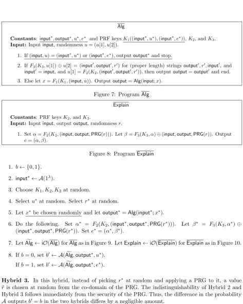
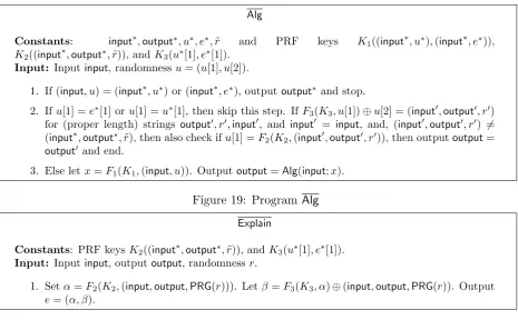
Hybrid 1. In this hybrid, we modify the Alg program as follows: First, we add constants

input∗,output∗, u∗, e∗ to the program. Then, we add an “if” statement at the start that outputs

output∗ if the input is either (input∗, u∗) or (input∗, e∗), as this is exactly what the original Alg

(19)

Alg

Constants: KeysK1,K2, andK3.

Input: Inputinput, randomnessu= (u[1], u[2]).

1. IfF3(K3, u[1])⊕u[2] = (input′,output′, r′) for (proper length) strings output′, r′,input′, and input′=input, andu[1] =F2(K2,(input′,output′, r′)), then outputoutput=output′ and end.

2. Else letx=F1(K1,(input, u)). Outputoutput=Alg(input;x).

Explain

Constants: KeysK2 andK3.

Input: Inputinput, outputoutput, randomnessr∈ {0,1}λ_.

1. Setα=F2(K2,(input,output,PRG(r))). Letβ=F3(K3, α)⊕(input,output,PRG(r)). Output e= (α, β).

Figure 6: Program Explain

By construction, the new Alg program is functionally equivalent to the original Alg program. Therefore the indistinguishability of Hybrid 0 and Hybrid 1 follows by the security of iO. Thus, the probabilities thatA outputsb′ =b in the two hybrids diﬀer by a negligible amount.

Note: Implicitly, all “if” statements that are added to programs with multiple checks are written in lexicographic order; that is, if u∗ < e∗ in lexicographic order, we write it as “If (input, u) = (input∗, u∗) or (input∗, e∗),” otherwise we write it as “If (input, u) = (input∗, e∗) or (input∗, u∗).”

1. b← {0,1}.

2. input∗ ← A(1λ).

5. Letx∗=F1(K1,(input∗, u∗)) and let output∗ =Alg(input∗;x∗).

Hybrid 2. Here, the valuex∗ is chosen uniformly instead of as the output ofF1(K1,(input∗, u∗)). The indistinguishability of Hybrid 2 from Hybrid 1 follows immediately from the pseudorandomness property of the punctured PRFF1 (Deﬁnition 2). Thus, the diﬀerence in the probabilityAoutputs

(20)

Alg

Constants: input∗,output∗, u∗, e∗ and PRF keysK1((input∗, u∗),(input∗, e∗)),K2, and K3. Input: Inputinput, randomnessu= (u[1], u[2]).

1. If (input, u) = (input∗, u∗) or (input∗, e∗), outputoutput∗ and stop.

Explain

Constants: PRF keysK2, and K3.

Input: Inputinput, outputoutput, randomnessr.

1. Setα=F2(K2,(input,output,PRG(r))). Letβ=F3(K3, α)⊕(input,output,PRG(r)). Output e= (α, β).

1. b← {0,1}.

2. input∗ ← A(1λ).

5. Letx∗ be chosen randomly and letoutput∗=Alg(input∗;x∗).

Hybrid 3. In this hybrid, instead of picking r∗ at random and applying a PRG to it, a value ˜

r is chosen at random from the co-domain of the PRG. The indistinguishability of Hybrid 2 and Hybrid 3 follows immediately from the security of the PRG. Thus, the diﬀerence in the probability A outputsb′=bin the two hybrids diﬀers by a negligible amount.

1. b← {0,1}.

2. input∗ ← A(1λ_).

(21)

Alg

Constants: input∗,output∗, u∗, e∗ and PRF keysK1((input∗, u∗),(input∗, e∗)),K2, and K3. Input: Inputinput, randomnessu= (u[1], u[2]).

3. Else letx=F1(K1,(input, u)). Outputoutput=Alg(input;x).

Explain

Constants: PRF keysK2, and K3.

1. Setα=F2(K2,(input,output,PRG(r))). Letβ=F3(K3, α)⊕(input,output,PRG(r)). Output e= (α, β).

4. Selectu∗ at random. Select ˜r at random.

6. Do the following. Setα∗ =F2(K2,(input∗,output∗,r˜)). Letβ∗=F3(K3, α∗)⊕(input∗,output∗,r˜). Sete∗= (α∗, β∗).

7. Let Algf ← iO(Alg) for Alg as in Figure 11. Let Explain ← iO(Explain) for Explain as in Figure 12.

Alg

Constants: input∗,output∗, u∗, e∗ and PRF keysK1((input∗, u∗),(input∗, e∗)),K2, and K3. Input: Inputinput, randomnessu= (u[1], u[2]).

(22)

Explain

Constants: PRF keysK2, and K3.

1. Setα=F2(K2,(input,output,PRG(r))). Letβ=F3(K3, α)⊕(input,output,PRG(r)). Output e= (α, β).

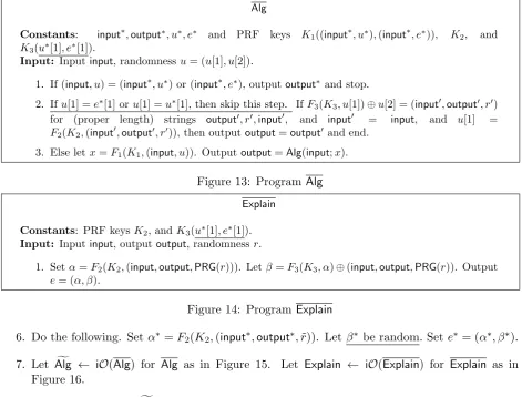
Hybrid 4. In this hybrid, theAlgandExplainprograms are modiﬁed as shown below. In Lemma 2, (proven below after all hybrids are given), we argue that except with negligible probability over choice of constants, these modiﬁcations do not alter the functionality of either program.

Thus, the indistinguishability of Hybrid 3 and Hybrid 4 follows from the iO security property. and so the diﬀerence in the probability A outputsb′ =bin the two hybrids diﬀers by a negligible amount.

1. b← {0,1}.

2. input∗ ← A(1λ_).

6. Do the following. Setα∗ =F2(K2,(input∗,output∗,r˜)). Letβ∗=F3(K3, α∗)⊕(input∗,output∗,r˜). Sete∗= (α∗, β∗).

7. Let Algf ← iO(Alg) for Alg as in Figure 13. Let Explain ← iO(Explain) for Explain as in Figure 14.

Hybrid 5. In this hybrid, the valuee∗[2], denotedβ∗, is chosen at random instead of being chosen asβ∗=F3(K3, α∗)⊕(input∗,output∗,r˜). The indistinguishability of Hybrid 4 and Hybrid 5 follows immediately from the pseudorandomness property of the puncturable PRFF3. Thus, the diﬀerence in the probabilityAoutputs b′=bin the two hybrids diﬀers by a negligible amount.

1. b← {0,1}.

2. input∗ ← A(1λ).