Remarks on Quantum Modular Exponentiation and Some Experimental Demonstrations of Shor's Algorithm

(1)

Remarks on Quantum Modular Exponentiation and

Some Experimental Demonstrations of Shor’s Algorithm

Zhengjun Cao1,∗_, _{Zhenfu Cao,}2,3 _{Lihua Liu}4

Abstract. An efficient quantum modular exponentiation method is indispensible for Shor’s factoring algorithm. But we find that all descriptions presented by Shor, Nielsen and Chuang, Markov and Saeedi, et al., are flawed. We also remark that some experimental demonstrations of Shor’s algorithm are misleading, because they violate the necessary condition that the selected number q = 2s_{, where} _s _{is the number of}

qubits used in the first register, must satisfyn2≤q <2n2, where nis the large number to be factored.

Keywords. Shor’s factoring algorithm; quantum modular exponentiation; super-position; continued fraction expansion.

1 Introduction

The problem of factoring integers is widely believed to be hard. The famous public key cryptosys-tem, RSA, is directly based on the difficulty of factorization. Notice that factoring an integerncan be reduced to finding the order of an integerx with respect to the module n (G. Miller [1]). The order is usually denoted by the notation ordn(x).So far, there is not a polynomial time algorithm

run on classical computers which can be used to compute ordn(x).

In 1994, P. Shor [2] proposed the first quantum algorithm which can compute ordn(x) in

poly-nomial time. The factoring algorithm requires two quantum registers. At the beginning of the algorithm, one has to find q = 2s _{for some integer} _s _{such that} _n2 _≤ _{q <} ₂_n2_{, where} _n _{is to be} factored. The followed steps are:

Initialization. Put register-1 in the following uniform superposition

1

√_q

q−1 X

a=0

|a_i|0_i.

1_{Department of Mathematics, Shanghai University, Shanghai, China.} ∗

[email protected] 2_{Department of Computer Science and Engineering, Shanghai Jiao Tong University, China.} 3_{Software Engineering Institute, East China Normal University, Shanghai, China.}

4_{Department of Mathematics, Shanghai Maritime University, Shanghai, China.}

(2)

Computation. Keep a in register-1 and compute xa _{in register-2 for some randomly chosen}

integerx. We then have the following state

1

√_q

q−1 X

a=0

|ai|xai.

Fourier transformation. Performing Fourier transform on register-1, we obtain the state

1 q

q−1 X

a=0

q−1 X

c=0

exp(2πiac/q)_|c_i|xa_i_.

Observation. It suffices to observe the first register. The probability p that the machine reaches the state_|c, xk_i _is

1 q

X

a:xa_≡_xk

exp(2πiac/q) 2

where 0_≤k < r= ordn(x), the sum is over all a(0≤a < q) such thatxa≡xk.

Continued fraction expansion. If there is adsuch that −r

2 ≤dq−rc≤ r2, then the probability of seeing|c, xk_i _{is greater than 1}_/₃_r2_{. Hence, we have}

d r −

c q ≤

1 2q.

:::::

Since_::::::::q ≥n2,_:::we_::::can_::::::round_::::c/q_:::to_::::::obtain_:::::d/r. Thus r can be obtained.

P. Shor has specified the operations for the process |0i|0i → √1

q

Pq−1

a=0|ai|0i, but not specified the operations for the process √1

q

Pq−1

a=0|ai|0i → √1q

Pq−1

a=0|ai|xa(modn)i.His original description specifies only the process (a,1)→ (a, xa_mod_n_{). Nielsen and Chuang in their book Ref.[3] specify}

that

|ai|yi → |aiUat−12t−1_{· · ·}_Ua020_|_y_i₌_|_a_i|_xat−12t−1 _{× · · · ×}_xa020_y_(mod_n₎_i₌_|_a_i|_xa_y_(mod_n₎_i where a’s binary representation is at−1at−2· · ·a0, U is the unitary operation such that U|yi ≡

|xy(modn)_i,y_{∈ {}0,1_}`_,_`_{is the bit length of} _n_.

We find the Nielsen-Chuang quantum modular exponentiation method requiresaunitary oper-ations. Apparently, it is inappropriate for the process

1

√_q

q−1 X

a=0

|a_i|0_{i →} _√1 q

q−1 X

a=0

|a_i|xa_(mod_n₎_i

(3)

Since 2001, some teams have reported that they had successfully factored 15 into 3_×5 using Shor’s algorithm. We shall have a close look at these experimental demonstrations and remark that these demonstrations are misleading, because they violate the necessary condition that the selected numberq must satisfyn2 _≤_{q <}₂_n2_.

2 Preliminaries

A quantum analogue of a classical computer operates with quantum bits involving quantum states. The state of a quantum computer is described as a basis vector in a Hilbert space. A qubit is a quantum state|Ψi of the form

|Ψ_i=a_|0_i+b_|1_i,

where the amplitudesa, b_∈Csuch that_|a_|2+_|b_|2 = 1,_|0_i and _|1_iare basis vectors of the Hilbert space. Here, theket notation_|x_imeans thatxis a quantum state. The state of a quantum system havingn qubits is a point in a 2n_{-dimensional vector space. Given a state}

2n₋₁

X

i=0

ai|χii,

where the amplitudes are complex numbers such that P2_i₌₀n−1|ai|2 = 1 and each |χii is a basis

vector of the Hilbert space, if the machine is measured with respect to this basis, the probability of seeing basis state|χii is|ai|2.

Two quantum mechanical systems are combined using the tensor product. For example, a system of two qubits_|Ψ_i=a1|0i+a2|1iand |Φi=b1|0i+b2|1i can be written as

|Ψi|Φi=

a1 a2

⊗

b1 b2

=

      

a1b1 a1b2 a2b1 a2b2

      

We shall also use the shorthand notations |Ψ,Φi. We call a quantum state having two or more components entangled state, if it is not a product state. According to the Copenhagen interpre-tation of quantum mechanics, measurement causes an instantaneous collapse of the wave function describing the quantum system into an eigenstate of the observable state that was measured. If entangled, one object cannot be fully described without considering the other(s).

Operations on a qubit are described by 2×2 unitary matrices. Of these, some of the most important are

X= "

0 1

1 0 #

, Y = "

0 ₋i

i 0 #

, Z = "

1 0

0 −1 #

, H = √1

2 "

1 1

1 −1 #

(4)

whereH denotes the Hadamard gate. Clearly, H_|0_i= √1

2(|0i+|1i).

Operations on two qubits are described by 4_×4 unitary matrices. Of these, the most important operation is the controlled-NOT, denoted by CNOT. The action of CNOT is given by |ci|ti → |c_i|c_⊕t_i, where_⊕denotes addition modulo 2. The matrix representation of CNOT is

      

1 0 0 0

0 1 0 0

0 0 0 1

0 0 1 0        .

Likewise,_::::::::::operations_:::on_::n_:::::::qubits_::::are_:::::::::described_:::by_::::::::2n_×₂n

::::::::unitary:::::::::matrices.

There is another method to describe linear operators performed onmultiple qubits. Suppose that V andW are vector spaces of dimension 2µ_{and 2}ν _{(they describe quantum systems corresponding}

toµ and ν qubits, respectively). Suppose |vi and |wi are vectors inV and W, and A and B are linear operators onV and W, respectively. Then we can define a linear operator A_⊗B onV _⊗W by the equation

(A⊗B)(|vi ⊗ |wi)≡A|vi ⊗B|wi.

3 Remarks on quantum modular exponentiation method

3.1 The Shor’s original description

P. Shor has specified the operations for the process

|0i|0i → √1_q

q−1 X

a=0

|ai|0i,

whereq = 2s _{for some positive integer} _s_{such that} _n2 _≤_{q <}₂_n2_, _n_{is to be factored. Notice that} the first register consists of s qubits. He wrote: “this step is relatively easy, since all it entails is putting each qubit in the first register into the superposition √1

2(|0i+|1i).” (This can be done using the Hadamard gatestimes.)

Shor has not specified the operations for the process

1

√_q

q−1 X

a=0

|ai|0i → √1_q

q−1 X

a=0

|ai|xa(modn)i.

(5)

follows.

The technique for computingxa_{(mod ) is essentially the same as the classical method.}

First, by repeated squaring we compute x2i

(mod ) for alli < l. Then, to obtainxa_{(mod )}

we multiply the powersxa_{(mod ) where 2}i _{appears in the binary expansion of} _a_{. In our}

algorithm for factoringn, we only need to compute xa_{(mod ) where} _a_{is in a superposition}

of states, but x is some fixed integer. This makes things much easier, because we can use a reversible gate array where ais treated as input, but wherex and nare built into the structure of the gate array. Thus, we can use the algorithm described by the following pseudocode; here,ai represents the ith bit ofain binary, where the bits are indexed from

right to left and the rightmost bit of aisa0. power:=1

for i= 0 to l₋1

if (ai == 1)then

power:=power ∗x2i(modn)

endif endfor

The variableais left unchanged by the code and xa_{(mod ) is output as the variable}_power_.

Thus, this code takes the pair of values (a,1) to (a, xa_{(mod )).}

Remarks on the Shor’s description:

• The description indicates only the conventional process

(a,1)→(a, xamodn), rather than the quantum process

|a_i|0_{i → |}a_i|xamodn_i, let alone the more complicated quantum process

1

√_q

q−1 X

a=0

|ai|0i → √1_q

q−1 X

a=0

|ai|xa(modn)i.

• Sinceai is required to computexa(modn) which represents theith bit ofain binary, one has

to measure the superposition √1

q

Pq−1

a=0|ai|0i to obtain a. But it is impossible to practically compose pure states

|a_i|xa_(mod_n₎_i_{, a}_{= 0}_,₁_,_{· · ·}_{, q}₋₁_,

into the superposition √1

q

Pq−1

a=0|ai|xa(modn)i,because q≥n2 and nis the large number to be factored.

• Although it specifies the Hadamard gate on each qubit in the first register,_::it_::::does_::::not_:::::::specify

::::

how_::::::many_::::and_:::::what_::::::::::quantum_:::::gates_:::or_::::::::unitary_::::::::::operations_::::are_:::::used_:::on_:::::each_::::::qubit_::or_::a_::::::group

::

(6)

3.2 The Nielsen-Chuang description

Nielsen and Chuang in their book Ref.[3] specify that

|ai|yi → |aiUat−12t−1_{· · ·}_Ua020_|_y_i₌_|_a_i|_xat−12t−1 _{× · · · ×}_xa020_y_(mod_n₎_i₌_|_a_i|_xa_y_(mod_n₎_i wherea’s binary representation isat−1at−2· · ·a0,U is the unitary operation such that

U_|y_{i ≡ |}xy(modn)_i,

y_{∈ {}0,1_}`_,_`_{is the bit length of} _n_{. They wrote:}

Using the techniques of Section 3.2.5, it is now straightforward to construct a reversible circuit with a t bit register and an`bit register which, when started in the state (a, y) outputs (a, xa_y_(mod_n_{)), using}_O₍_`3_{) gates, which can be}

translated into a quantum circuit using O(`3) gates computing the transformation

|ai|yi → |ai|xa_y_(mod_n₎_i_.

Although they indicate that the classical circuit for the conventional process

(a, y) O(`

3₎_{classical gates}

− − − − − − − −→(a, xa_y_(mod_n₎₎

can be translated into a quantum circuit for the quantum process

|ai|yiO(`

3₎_{quantum gates}

− − − − − − − −→ |ai|xay(modn)i,

we now want to remark that the quantum circuit has to invoke U, the unitary operation, atimes. Thus, the wanted process

1

√_q

q−1 X

a=0

|a_i|0_{i →} _√1 q

q−1 X

a=0

|a_i|xa_(mod_n₎_i

has to invoke the unitary operation 1 + 2 +_{· · ·}+ (q₋1) _≈ O(q2_{) times, if all terms} _|_a_i|₀_i_, _a ₌ 0,· · · , q−1, are processed one by one. Even worse, the transformation for the process

|q₋1_i|y_{i → |}a_i|xq−1_y_(mod_n₎_i

has to invoke the unitary operationq₋1 times according to the Nielsen-Chuang description. Clearly,

:

it_::::can_::::not_:::be_{::::::::::::::}accomplished_::in_::::::::::::polynomial_:::::time_::::::::because_:q_:::is_::a_:::::large_::::::::number.

3.3 The Markov-Saeedi quantum circuit

(7)

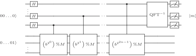
H · · · •

QFT−1 .

. .

|00. . .0i H • · · · |mi

H • · · ·

b20_%_M _b21_%_M

· · ·

b22n−1%M

|0. . .01i · · ·

. .

. _{· · ·}

Figure 1: An outline of the quantum part of Shor’s algorithm.

1.1 Shor’s algorithm

Shor’s algorithm seeks to factor a given value M > 0, which we assume to be semiprime M =pq with unknown factors. The strategy is to consider the functions fb(x) = xb%M2, potentially with several

different 1 < b < M values and determine their periods in case gcd(b, M) = 1. When the period is determined to be even b2π_%_M _{= 1, we have (}_bπ ₋₁₎₍_bπ_{+ 1)%}_M _{= 0, thus either (}_bπ₋_{1) or (}_bπ _{+ 1)}

must share at least one prime factor with M. If bπ_%_M ₆₌ ₋_{1, such a factor can be found using}

gcd(bπ±1, M), otherwise it leads to the trivial factors 1 and M. When the period is determined to be odd, another b value is tried.

The period-finding procedure relies on a quantum circuit (Figure 1), instantiated for a given value 1 < b < M coprime with M. The circuit operates on two 0-initialized quantum registers [15] with

• a block of parallel Hadamard gates on Register 1,

• a circuit for modular exponentiation (mod-exp) evaluates f(y) = by_%_M _{by mapping} _|_y_i|₀_{i 7→}

|y_i|f(y)_i, where y is read from Register 1 and f(y) is written to Register 2; Register 1 can be temporarily modified, but must be restored at the end,

• a circuit for the Quantum Fourier Transform (QFT) on Register 1,

• a block of parallel measurements on Register 1.

The first and last blocks cannot be optimized any further. QFT circuits are understood fairly well and are much smaller than circuits for modular exponentiation [15]. Therefore, our focus is on mod-exp circuits. They typically consist of reversible gates — NOT (N), CNOT (C) and Toffoli (T) — which can be modeled and optimized entirely in terms of Boolean logic [17]. However, in physical implementations, Toffoli gates must be decomposed into smaller gates directly implementable in a given technology [18]. Reversible circuits for modular exponentiation start with an inverter on Register 2 that changes the

|000· · ·0i value to |000· · ·1i, and otherwise exhibit the following structure: each (i-th) bit of Register 1 enables (controls) a circuit block that multiplies Register 2 by Ci = b2

i

%M and reduces the result %M. When b and M are known, Ci can be pre-computed without quantum computation. Therefore, we refer to Cix%M-blocks below. They are typically implemented using shift and addition circuits, and a number of relevant quantum adders are known [9, 19]. The selection of appropriate adder types is discussed in [20, 10].

Each controlled modular multiplication is traditionally implemented separately. When dealing with reversible logic and quantum circuits, we note that the coprimality of C and M makes x 7→ Cx%M a reversible transformation. The number of coprimeC values is ϕ(M) = (p₋1)(q₋1), where ϕ(M) is the Euler’s totient function and gives the size of (Z/MZ)× — the multiplicative group of integers mod-M. For M = 15, modular multiplication circuits for the eight C coprime values are illustrated in Figure 2. Figure 3 shows circuits for f(x) =bx_{%15, gcd(}_b,_{15) = 1.}

When not knowing p and q, one should also not assume any knowledge that would make it easy to find them. For example, one should not choose C that satisfies C2π _{= 1%}_M _{with a known (small)} _π

because such solutions would allow one to factorize M via gcd(Cπ±1, M). Also recall that (Z/MZ)× is a product of two cyclic groups Z/pZ and Z/qZ, and thus (Z/MZ)× admits a generating set with only two elements. However, knowing such generators is tantamount to knowing p and q. When working with specific small M =pq, it is sometimes difficult to avoid using the knowledge of p and q, but results obtained this way do not necessarily scale to large values. The same can be said about results produced through exhaustive search.

2_{Here and in the remaining text, the percent sign % denotes the modulo (remainder) operation, as it does in the C and}

C++ languages.

The Markov-Saeedi quantum circuit for modular exponentiation is flawed, too. The unitary matrix corresponding to (b2i)%M for some integeri, which is performed on all qubits in the sec-ond quantum registers, has a tremendous dimension (not less than the modularM). To implement the operator practically,_:::one_::::::must_:::::::::::decompose_::it_:::::into_::::the_::::::tensor_:::::::::product_::of_::::::some_::::::linear_::::::::::operators

::::

with_::::low_:::::::::::dimension. Regretfully, they had not specified these low dimension linear operators at all.

Moreover, they had not specified the output of the operator (b20)%M . We now want to ask:

(1) what are the inputting states of the unitary operator (b22n−1)%M ?

(2) how to decompose the operator (b22n−1)%M into the tensor product of some low di-mension linear operators?

(3)_::::how_::::::many_:::::::::::executable_::::::::unitary_:::::::::operators_::::are_:::::::::required in the quantum modular exponenti-ation process?

In our opinion, their proposed quantum circuit for modular exponentiation is incorrect and mis-leading.

3.4 On Scott Aaronson’s explanation

We have reported the flaw to some researchers including P. Shor himself, but only received a comment made by MIT professor Scott Aaronson. He explained that (personal communication, 2014/09/02):

The repeated squaring algorithm works (and works in polynomial time) for any single |ai|0i, mapping it to|ai|xa_(mod_n₎_i_{. But, because of the}

linearity of quantum mechanics, this immediately implies that the algorithm

must also work for any superposition of _|a_i’s, mappingP_a_|a_i toP_a_|a_i|xa_(mod_n₎_i_.

We do not think that his answer is convincing, because it is too vague to specify how many and what quantum gates or unitary operations are used on each qubit or a group of qubits in the second quantum register. Besides, according to the Nielsen-Chuang description, the process

(8)

depends on the binary representation of the exponenta. Which integer should be extracted in the superposition √1

q

Pq−1

a=0|ai|0i for computing the wanted state √1q

Pq−1

a=0|ai|xa(modn)i? He did not pay more attentions tothe difference between two linear operators performed on a pure state and a superposition.

4 It is difficult to modulate the wanted state in the second register

We know the wanted superposition in the first register is modulated by the following procedure.

First, a Hadamard gateH= √1

2 "

1 1

1 ₋1 #

is performed on each qubit to obtain thesintermediate

states of √1

2(|0i+|1i). Second, combine all these states using the tensor product. 1

√

2(|0i+|1i)⊗ 1

√

2(|0i+|1i) = 1

2(|00i+|01i+|10i+|11i) 1

√

2(|0i+|1i)⊗ 1

√

2(|0i+|1i)⊗ 1

√

2(|0i+|1i)

= 1

2√2(|000i+|001i+|010i+|011i+|100i+|101i+|110i+|111i) ..

. 1

√

2(|0i+|1i)⊗ · · · ⊗ 1

√

2(|0i+|1i)

| {z }

squbits

= _√1 q

q−1 X

a=0

|ai

Note that the procedure works well because all those involved pure states are in binary form. We would like to stress that if two pure states are in decimal representations|xi,|x2i, then we can not directly combine them to obtain |x3i. Suppose that the binary strings for integers x, x2 arebk· · ·b0,b0i· · ·b00. We have

|x_{i ⊗ |}x2_i=_|bk· · ·b0b0i· · ·b00i=|2i+1x+x2i. Thus,

1

√

2(|1i+|xi)⊗ 1

√

2(|1i+|x

2_(mod_n₎_i₎_{⊗ · · · ⊗}_√1 2

|1i+|x2s−1(modn)i6= _√1 q

q−1 X

a=0

|xa(modn)i, whereq= 2s_{, although there is a corresponding conventional equation}

(1 +x)(1 +x2)(1 +x22)· · ·(1 +x2s−1) =

q−1 X

a=0 xa. ::

It_::::::seems_:::::that_::::::some_:::::::people_:::are_:::::::::confused_::::by_::::the_::::::above_:::::::::equation_::::and_::::::::simply_::::take_::::for_::::::::granted_:::::that

:::::::::

(9)

5 On some experimental demonstrations of Shor’s algorithm

In 2001, it is reported that Shor’s algorithm was demonstrated by a group at IBM, who factored 15 into 3_×5, using a quantum computer with 7 qubits,3 qubits for the first register and 4 qubits for the second register (see Figure-2) [6].

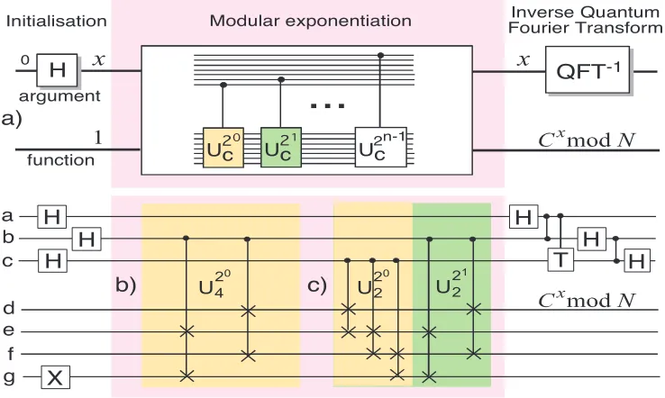
In 2007, a group at University of Queensland reported an experimental demonstration of a compiled version of Shor’s algorithm. They factored 15 into 3_×5, using 7 qubits either, 3 qubits for the first register and 4 qubits for the second register (see Figure-3) [7].

In 2007, a group at University of Science and Technology of China reported another experimental demonstration of a complied version of Shor’s algorithm. They factored 15 into 3_×5 using6 qubits only,2 qubits for the first register and 4 qubits for the second register (see Figure-4) [8].

In 2012, a group at University of California, Santa Barbara, reported a new experimental demonstration of a compiled version of Shor’s algorithm. They factored 15 into 3×5 using3 qubits either,1 qubits for the first register and 2 qubits for the second register (see Figure-5) [9].

Demonstrations qubits used in the first register qubits used in the second register

Figure 2, Ref.[6] 3 4

15

Figure 1

L. Vandersypen NATURE 07-Sep-01

inverse

QFT

a v e r a g i n g l ar o p me

t 1:

3: 2:

4: 5: 6: 7:

0

1

90

A _F _G _H

90 45 H

H H

H

b. a.

m

1

x x

mod

x a n

H n

B C D E

N

(3) (4)

(2) (1)

(0)

a.

(10)

2 application of the order-finding function produces the

entangled state

P

2_xn₌₀−1

_|

x

_i|

C

x

mod

N

_i

; iii) the

inverse

Quantum Fourier Transform

(QFT) followed by

mea-surement of the argument-register in the logical basis,

which with high probability extracts the order

r

after

fur-ther classical processing. If the routine is standalone, the

inverse QFT can be performed using an approach based

on local measurement and feedforward [21]. Note that

the inverse QFT in [14] was unnecessary: it is

straight-forward to show this is true for any order-2

l

circuit [22].

Modular exponentiation is the most

computationally-intensive part of the algorithm [13]. It can be realised by

a cascade of controlled unitary operations,

U

, as shown

in the nested inset of Fig. 1a). It is clear that the

reg-isters become highly entangled with each other: since

U

is a function of

C

and

N

, the entangling operation is

unique to each problem. Here we choose to factor 15 with

the first two co-primes,

C

=2 and

C

=4. In these cases

en-tire sets of gates are redundant: specifically,

U

2n

=

I

when

x

1 H Uc2 0 Uc2 1 Uc2n-1 QFT-1

...

b) H H a b c d e f g H H H a b c d e argument function 0 x a b c d e f g _X H T H H H H H H c) d) e) f) g) U2 0 4 U2 0 4 U2 0 4 U2 0 2 U 21 2 U2 0 2 U2 0 2 U2 1 2 U2 1 2 X X a) C

Initialisation Modular exponentiation _{Fourier Transform}Inverse Quantum

x x x H H H T H H H T

FIG. 1: a) Conceptual circuit for the order-finding routine of

Shor’s algorithm for number

N

and co-prime

C

[13]. The

ar-gument and function registers are bundles of

n

and

m

qubits;

the nested order-finding structure uses

U

|

y

i

=

|

Cy

mod

N

i

,

where the initial function-register state is

|

y

i

=1. The

algo-rithm is completed by logical measurement of the

argument-register, and reversing the order of the argument qubits. b),c)

Implementation of a) for

N

=15 and

C

=4

,

2, respectively; the

unitaries are decomposed into controlled-

swap

gates (

cswap

),

marked as

x

; controlled-phase gates are marked by dots;

h

and

t

represent Hadamard and

π/

8 gates. Many gates are

redun-dant, e.g. the second gate in b), the first and second gates in

c). d),e) Partially-compiled circuits of b),c), replacing

cswap

by controlled-

not

gates. n.b. e) is equivalent to the

N

=15

C

=7 circuit in Ref.[14]. f),g) Fully-compiled circuits of d),e),

by evaluating log

_C

[

C

x

mod

N

] in the function-register.

n>

0 for

C

=4, and

U

2n

=

I

when

n>

1 for

C

=2. Figs 1b),c)

show the remaining gates for

C

=4 and

C

=2, respectively,

after decomposition of the unitaries into controlled-

swap

gates—this level of compiling is equivalent to that

in-troduced in Ref. [14].

Further compilation can always

be made since the initial state of the function-register

is fixed, allowing the

cswap

gates to be replaced by

controlled-

not

(

cnot

) gates as shown in Figs 1d),e) [23].

We implemented the order-2-finding circuit, Fig. 1d).

The qubits are realised with simultaneous forward and

backward production of photon pairs from parametric

downconversion, Fig. 2a): the logical states are encoded

into the vertical and horizontal polarisations. This circuit

required implementing a recently-proposed three-qubit

quantum-logic gate, Fig. 2b), which realises a cascade of

n

controlled-

z

gates with exponentially greater success

than chaining

n

individual gates [24].

The

controlled-not

gates are realised by combining Hadamards and

controlled-

z

gates based on partially-polarising

beam-splitters. The gates are nondeterministic, with one third

success probability when fully prebiased [8, 9, 10]. A run

of each routine is flagged by a fourfold event, where a

single photon arrives at each output.

Dependent

pho-tons from the forward pass interfere non-classically at

V H F1 F2 B2 B1 F1 F2 B1 F1 F2 B1 B2 V H H V H V V H a) b) _c) V H H V H V H V Laser d) e) F1 F2 B1 1/3 F1 F2 B1 B2

R_V=1/3 R_H=1

! RV=1

R_H=0

! ! ! "/2 "/4 b e g b c d e b e g b c d e 1/3 1/3 1/3 SHG PDC

FIG. 2: Experimental schematic. a) Forward and backward

photons pairs are produced via parametric downconversion

(PDC) of a frequency-doubled mode-locked Ti:Sapphire laser

(820 nm

_→

410 nm, ∆

τ

=80 fs at 82 MHz repetition rate)

through a Type-I 2 mm Bismuth Borate (BiB

3

O

6

) crystal.

Photons are input to the circuits via blocked interference

filters (820

±

3 nm) and single-mode optical fibres, and

de-tected using single photon counting modules, (PerkinElmer

AQR-14FC). Coincidences are measured using a quad-logic

card driven by a four-channel constant fraction

discrimina-tor. With 500 mW at 410 nm this yielded 60 kHz and 25 kHz

twofold coincidence rates for direct detection, which differed

due to mismatched pump focus sizes; the measured fourfold

coincidence rate was 35 Hz. b),c) Linear optical circuits for

order-2 and order-4 finding algorithms, with inputs from a)

labelled; the letters on the detectors refer to the Fig. 1 qubits.

d),e) Physical optical circuits for b),c), replacing the classical

interferometers with partially-polarising beamsplitters.

Figure 3: Conceptual circuit for Shor’s algorithm for numberN = 15 and co-primeC = 4.

2 a) b) n m n n c) Z PBS PBS HWP CNOT 1 2 3 4 3 1 4 2

FIG. 1: Quantum circuit for the order-finding routine of Shor’s algorithm. (a). Outline of the quantum circuit. (b). Quantum circuit for N = 15 and a = 11. The MEF is implemented by two CNOT gates and the QFT is implemented by Hadamard rotations and two-qubit conditional phase gates. The gate-labeling scheme denotes the axis about which the conditional rotation takes place and the angle of rotation. (c). The simplified linear optics network using HWPs and PBSs to implement the MEF circuit and the semiclassical version of the QFT circuit. The double lines denote classical information.

Implementations of this algorithm, even for factoriza-tion of a small number, place a lot of challenging exper-imental demands, e.g., coherent manipulations of multi-ple qubits and creations of highly-entangled multiqubit registers. Here we aim to demonstrate the simplest in-stance of Shor’s algorithm, i.e., the factorization of 15. Quantum networks for evaluating the MEF have been designed which involve O(n3) operations [15, 17]. Since ax =a2n−1xn−1· · ·_a2x1_ax0_{, the execution of MEF can be} decomposed into a sequence of controlled multiplications. A general purpose algorithm to factorize 15 would require at least n= 8, m = 4, thus total 12 qubits [15]. Several observations allow us to reduce the resources substan-tially for the purpose of a proof-of-principle demonstra-tion. First we choose to implement the algorithm with a= 11, this was identified in [5] as the “easy” case. Since a2mod15 = 1, MEF can be simplified to multiplications controlled only by x0, which can be implemented by two controlled-NOT (CNOT) gates [18]. A QFT then fol-lows to read out the period r. Such a circuit is shown in Fig. 1b. We note there are two qubits in the second reg-ister which evolve trivially during computation and can thus be left out.

To demonstrate the circuit of Fig. 1b we use single pho-tons as qubits, where _|0_i and _|1_i are encoded with the photon’s horizontal (H) and vertical (V) polarization re-spectively. The difficulty in implementing this circuit lies in the CNOT gates and conditionalπ/2-phase shift gate. Although such entangling gates are possible for photons in principle using measurement-induced nonlinearity [7], currently they are still experimentally expensive [9, 19]. Here we note that since the target qubits of the CNOT gates are always fixed at _|H_i, so the gate could be re-alized in an easier and more efficient fashion. Such a CNOT gate use only a polarizing beam splitter (PBS) and a half-wave plate (HWP), through which an arbi-trary control qubit (α_|H_i+β_|V_i) and the target qubit

|Hi evolve into α|Hi|Hi+β|Vi|Vi upon post-selection [20], that is, conditioned on that there is one and only one photon out of each output (see Fig. 1c). Furthermore, the

QFT circuit can also be implemented with a more effi-cient method. It was observed by Griffiths and Niu [21] that when immediately followed by measurements, the fully coherent QFT can be replaced by a semiclassical version that employs only single-qubit rotations condi-tioned on measurement outcomes. This eliminates the need for entangling gates and reduces the numbers of gates quadratically. Thus we finally arrive at the simpli-fied linear optics MEF and QFT network in Fig. 1c. We note despite of these simplifications, our circuit suffices to demonstrate the underlying principles of this algorithm. Now we proceed with the experimental demonstration. Our experimental set-up is illustrated in Fig. 2, where a pulsed ultraviolet laser passes through two β-barium borate (BBO) crystals to create two pairs of entangled photon [22]. We use polarizers to disentangle the photons and prepare them in the states _|H_ii with i denoting the

spatial modes (see Fig. 1c). The photons pass through the HWPs and are superposed on the PBSs (see Fig. 2) to implement the necessary single- and two-qubit gates. To ensure good spatial and temporal overlap, the photons are spectrally filtered (∆λFWHW = 3.2 nm) and coupled by single-mode fibers [23].

How could one experimentally verify a valid demon-stration of Shor’s algorithm? First let us see the the-oretical predictions. After a = 11 is chosen, the first step of this algorithm, the MEF should evolve as (1/2)P3_x₌₀_|x_i|11x_mod15_i _{= (1}_/₂₎₍_|₀_i|₁_i₊_|₁_i|₁₁_i₊ |2_i|1_i+_|3_i|11_i).As we rewrite it in binary representation (|000001i+|011011i+|100001i+|111011i)/2, it shows that a nontrivial Greenberger-Horne-Zeilinger (GHZ) [24] entangled state |ψi = (1/√2)(|0i2|0i3|0i4+|1i2|1i3|1i4) is created between the two registers. For Shor’s algo-rithm as well as some others, multiqubit entanglement is a necessary condition if the quantum algorithm is to offer an exponential speed-up over classical computation [6]. In our experiment, as the photons pass through the MEF circuit, we first observe the Hong-Ou-Mandel type inter-ference [25] of three photons in arms 2-3-4 (see Fig. 3b). Then, after fixing the delays at the zero positions, we ex-Figure 4: Outline of quantum circuit for Shor’s algorithm for N = 15 and a= 11.

4 g "1" "0" h "1" "0" e ggg eee ggg eee 0 1/2 2 GHZ gg ee ee gg 1/2 0 -1/2 1 d H Q2 Q3 H H Cz H

armod(N)

Init Quantum Fourier Transform Modular Exponentiation H H H H

C_π_/2 Q2 Q3 Q4 Q1 |0> |0> |0> |0> H H Q2 Q3 Q4 |0> |0> |0> "0" "1" a

b 1 2 3

"00" "10" c i "1" "0" 0 1 0 1 1/2 0 1 3 f 1/4 0 ggg eee ggg eee -1/4 0

1 0 1 1/2 0

1 0

1 0 1 1/2 0

1

ψ_s

ψ₃

FIG. 3: Compiled version of Shor’s algorithm. a, Four-qubit circuit to factor N = 15, with co-prime a = 4. The three steps in

the algorithm are initialization, modular exponentiation, and the quantum Fourier transform, which computes ar_{mod(N) and}

returns the period r = 2. b, “Recompiled” three-qubit version of Shor’s algorithm. The redundant qubit Q1 is removed by

noting that HH = I. Circuits a and b are equivalent for this specific case. The three steps of the runtime analysis are labeled

1,2,3. c, CNOT gates are realized using an equivalent controlled-Z (CZ) circuit. d, Step 1: Bell singlet between Q2 and Q3

√

2 between

Q2, Q3, and Q4 with fidelity FGH Z =hGH Z|ρGH Z|GHZi = 0.59±0.01. f, Step 3: QST after running the complete algorithm.

density matrix of the single-qubit output register Q2 formed by: (g), tracing-out Q3 and Q4 from f, and (h) directly measuring

Q2 with QST, both with F = √ρ σm√ρ = 0.92±0.01 and SL = 0.78. From 1.5×105 direct measurements the output register

returns the period r = 2, with probability 0.483 ± 0.003, yielding the prime factors 3 and 5. (i), The density matrix of the

single-qubit output register without entangling gates, H2H2|gi = I|gi. The algorithm fails and returns r = 0 100 % of the

time. Compared to the single quantum state |ψouti = |gi, the fidelity Fcheck = hψg|ρcheck|ψgi = 0.83±0.01, which is less than

unity due to the energy relaxation.

“10” (including the redundant qubit) with equal proba-bility, where the former represents a failure and the latter indicates the successful determination of r = 2. We use three methods to analyze the output of the algorithm: Three-qubit QST, single-qubit QST, and the raw proba-bilities of the output register state. Figures 3g, h are the real part of the density matrices for the single qubit out-put register from three-qubit QST and one-qubit QST with fidelity F = √ρ σm√ρ = 0.92 ±0.01 for both

den-sity matrices. From the raw probabilities calculated from 150,000 repetitions of the algorithm, we measure the out-put “10” with probability 0.483 _±0.003, yielding r = 2, and after classical processing we compute the prime fac-tors 3 and 5.

The linear entropyS = 4[1₋Tr(ρ2_)]_/_{3 is another}

met-state, where SL = 1 for a completely mixed state[30]. We

find SL = 0.78 for both the reduced density matrix from

the third step of the runtime analysis (three-qubit QST), and from direct single-qubit QST of the register qubit.

As a final check of the requisite entanglement, we run the full algorithm without any of the entangling oper-ations and use QST to measure the single-qubit output register. The circuit reduces to twoH-gates separated by the time of the two entangling gates. Ideally Q2 returns

to the ground state and the algorithm fails (returns “0”) 100 % of the time. Figure 3i is the real part of the density matrix for the register qubit after running this check ex-periment. The fidelity of measuring the register qubit in

|g_i is Fcheck = hg|ρcheck |gi = 0.83±0.01. The algorithm

fails, as expected, without the entangling operations. Figure 5: A three-qubit compiled version of Shor’s algorithm to factorN = 15.

(11)

We now want to remark that:

• All these demonstrations are flawed because they violate the necessary condition that 152 < 28 _<₂_×₁₅2_,

:::::

which_:::::::means_::8_:::::::qubits_:::::::should_:::be_:::::used_::in_::::the_:::::first_::::::::register. Obviously, the last step of continued fraction expansion in Shor’s algorithm can not be accomplished if less qubits are used in the first register. It seems that these groups have misunderstood the necessary condition thatn2≤q <2n2 in Shor’s algorithm.

• In Figure 3, it directly denotes the output of the second register by Cx _mod _N_{. Clearly,}

the authors confused the numberCx _mod _N _{with the state}_|_Cx _mod _N_i_{. By the way, the}

wanted state in the second register is the superposition √1

8 P7

x=0|Cx mod Niinstead of the pure state_|Cx _mod _N_i_.

• In Figure 5, only 3 qubits are used. Clearly, the modular 15 can not be represented by the 3 qubits. In such case, how to ensure that the modular is really involved in the computation? In our opinion, the demonstration is unbelievable.

6 Conclusion

Shor’s factoring algorithm is interesting. But its subroutine for quantum modular exponentiation is not specified. We remark that both the Shor’s original description and the Nielsen-Chuang de-scription for quantum modular exponentiation are flawed. They can be used only for the pure state

|a_i|0_i, not for the superposition √1

q

Pq−1

a=0|ai|0i. We also remark that some experimental demon-strations of Shor’s algorithm are meaningless and misleading because they violate a necessary condition for Shor’s algorithm.

Acknowledgements. This work was supported by the National Natural Science Foundation of China (Grant Nos. 60970110, 60972034), and the State Key Program of National Natural Science of China (Grant No. 61033014).

References

[1] Miller G.: Riemann’s hypothesis and tests for primality. J. Comput. System Sci., 13: 300-317 (1976)

[2] Shor P.: Polynomial-time algorithms for prime factorization and discrete logarithms on a quantum computer. SIAM J. Comput. 26 (5): 1484-1509 (1997)

[3] Nielspen M., and Chuang I.: Quantum Computation and Quantum Information. Cambridge University Press (2000)

[4] Markov I., and Saeedi M.: Constant-Optimized Quantum Circuits for Modular Multiplication and Ex-ponentiation. Quantum Information and Computation, Vol. 12, No. 5&6, pp. 361-394 (2012)

[5] Markov I., and Saeedi M.: Faster Quantum Number Factoring via Circuit Synthesis, Physical Review A 87, 012310 (2013)

(12)

[7] Lanyon B., et al.: Experimental Demonstration of a Compiled Version of Shor’s Algorithm with Quantum Entanglement”, Physical Review Letters 99 (25): 250505. arXiv:0705.1398 (2007)

[8] Lu Chao-Yang, et al.: Demonstration of a Compiled Version of Shor’s Quantum Factoring Algorithm Using Photonic Qubits, Physical Review Letters 99 (25): 250504, arXiv:0705.1684 (2007)