COMPUTATIONAL STUDY OF FAST METHODS FOR THE EIKONAL EQUATION∗
PIERRE A. GREMAUD† AND CHRISTOPHER M. KUSTER†
Abstract. A computational study of the fast marching and the fast sweeping methods for the eikonal equation is given. It is stressed that both algorithms should be considered as “direct” (as opposed to iterative) methods. On realistic grids, fast sweeping is faster than fast marching for problems with simple geometry. For strongly nonuniform problems and/or complex geometry, the situation may be reversed. Finally, fully second order generalizations of methods of this type for problems with obstacles are proposed and implemented.
Key words. Hamilton–Jacobi, eikonal, viscosity solution, fast marching, fast sweeping
AMS subject classifications. 65N06, 65Y20, 49L25, 35F30
DOI.10.1137/040605655
1. Introduction. Steady state Hamilton–Jacobi equations play a major role in countless applications. While thediscretizationof those equations is approaching maturity (at least for single equations and convex Hamiltonians), the resolutionof the nonlinear discretized systems is an active topic of research.
In this paper, two methods are compared: the fast marching (FM) method [13, 14, 17] and the fast sweeping (FS) method [4, 8, 16, 19]. The two-dimensional eikonal equation is taken as a test problem: given a slowness fieldF (a positive function), we look for a time of propagationusatisfying
| ∇u|=F in Ω⊂R2,
(1.1)
u= 0 on Γ⊂R2.
(1.2)
The two-dimensional domain Ω is the computational domain; Γ is a source, i.e., a closed subset of ¯Ω in which u is zero. The slowness field F can be unbounded, corresponding to the presence of obstacles.
We refer the reader to [8, 15] for issues related to the application of the above methods to the more general problem
H(x,∇u) =F.
(1.3)
While clearly of importance, those considerations are related more to discretization than they are to resolution and are not the focus of this paper. Discretization algo-rithms are only briefly reviewed in section 2. In section 3, three nonlinear solvers are described (Gauss–Jacobi, FM, and FS/nonlinear Gauss–Seidel). Section 4 presents an adaption of the FM and FS methods to problems with obstacles. The relative efficiency of FM and FS is discussed in section 5. Concluding remarks are offered in section 6.
∗Received by the editors March 25, 2004; accepted for publication (in revised form) February 4, 2005; published electronically February 3, 2006.
http://www.siam.org/journals/sisc/27-6/60565.html
†Department of Mathematics and Center for Research in Scientific Computation, North Carolina State University, Raleigh, NC 27695-8205 ([email protected], [email protected]). The work of the first author was partially supported by National Science Foundation grants DMS-0204578, DMS-0244488, and DMS-0410561. The work of the second author was partially supported by Na-tional Science Foundation grant DMS-0244488.
2. Discretization. The basic construction principles for numerical Hamiltoni-ans are well known [10] and are easily described on a Cartesian grid. There, the basic scheme takes the form
H(Dx+Uij, D−xUij;D+yUij, Dy−Uij) =Fij, (2.1)
with the obvious notation. In that case, we recall thatHis consistent if
H(p, p;q, q) =H(p, q) ∀p, q,
(2.2)
where H is the Hamiltonian of the problem under consideration (here H(p, q) =
p2+q2). The numerical Hamiltonian is monotone if nonincreasing in its first and third arguments and nondecreasing in the other two: H(↓,↑,↓,↑) [6]. Consistency ensures that the correct problem is approximated while monotonicity guarantees con-vergence to the correct viscosity solution [5, 12].
Many numerical Hamiltonians can be found in the literature; most of them are derived from corresponding numerical fluxes for conservation laws. The main exam-ples are the Godunov fluxHG and the Lax–Friedrichs fluxHLF, which here take the form
HG(p
+, p−;q+, q−) =
max{p+−, p−+}2+ max{q+ −, q−+}2,
HLF(p
+, p−;q+, q−) =
p++p− 2
2 +
q++q− 2
2
−σx
p+−p− 2 −σy
q+−q−
2 ,
where σx ≥ max|∂H∂p| and σy ≥ max|∂H∂q|, where (·)+ = max{·,0} and (·)− = −min{·,0}. Upwind discretizations such as the Godunov method are especially sim-ple to imsim-plement for (1.1) and for convex Hamiltonians in general. However,HG, for instance, becomes very involved for general Hamiltonians. While centered methods such as Lax–Friedrichs do not suffer from that problem, they require special treatment at the boundary of the computational domain [8]. The discretization used below is essentiallyHG.
Many applications call for the use of non-Cartesian or unstructured meshes; see [1, 7, 9, 14, 15] for a few examples of such methods. Following [14, 15], consider a node
X0 at which the solutionU is to be computed and two neighboring nodesX1 andX2 at which the values ofU (U, = 1,2) and its derivatives (∂xU, ∂yU, = 1,2) are known or have already been computed. We set
N=
X0−X |X0−X|
, = 1,2, and N =
N1
N2
,
where N is a 2×2 nonsingular matrix, assumingX0,X1, and X2 are not lined up. The directional derivatives in the directionsN1 andN2 are approximated by
DU =
U0−U |X0−X|
, = 1,2 (first order formula), (2.3)
DU = 2
U0−U |X0−X|
Those approximate directional derivatives are linked to the gradient by
DU =N· ∇U +O(|X0−Xi|α) or DU =N ∇U+O(hα), (2.5)
whereDU = [D1U, D2U], h= max{|X0−X1|,|X0−X2|}, andα= 1 or 2 depending on whether (2.3) or (2.4), respectively, is used. Solving for ∇U and plugging into (1.1), one finds the (quadratic) equation defining the unknownU0,
DUt(N Nt)−1DU = (F(X0))2. (2.6)
The above methods are well understood theoretically: convergence to the viscosity solution when the Godunov fluxHG is used was established in [12]; see also [15] for additional results and references.
3. Resolution. The system of coupled quadratic equations corresponding to imposing (2.6) at all nodes has to be solved. Ifθdenotes the angles between N1and
N2, the matrixN Ntis symmetric positive definite provided 0< θ < π; its condition number is 1+cosθ
1−cosθ. Therefore, regardless of the choice of stencil (first or second order), (2.6) has two real solutions. This situation is generic for Hamilton–Jacobi equations. Let (U1, U2, . . . , UN) be the unknowns for an arbitrary ordering of the nodes. The resulting system can be written symbolically as
f(U) =f(U1, U2, . . . , UN) = 0. (3.1)
An iterative scheme, essentially a fixed point method or Gauss–Jacobi method, was proposed in [12]. One step of the algorithm is as follows.
Gauss–Jacobi algorithm.
• Choose a node and regard the neighboring values as fixed.
• Solve (2.6) for the value at the considered node; the largest of the two possible solutions is selected, in agreement with the viscosity criterion.
• Repeat until convergence (fixed point).
The corresponding pseudocode is k=0
U0= (0, . . . ,0)
while Uk=Uk+1 or k=0 k=k+1
for =1 to N solve f(Uk−1
1 , . . . ,U k−1
−1,U k
,Uk+−11, . . . ,U k−1
N ) =0 for U k
end
end
This approach is obviously slow, as each node has to be revisited several times before the numerical solution settles down. Further, no advantage is taken of the propagation character of the problem.
Fast Marching algorithm.
• The node with lowest value in the “front” set is removed from it and added to the “computed” set; its not-yet-computed neighbors are added to the “front.” • The values of all the nodes in the “front” are recomputed using (2.6). • Repeat until all the nodes are “computed.”
The list operations are handled by the heap sort algorithm [3, 18], which is the key to the speed of FM. This type of sort has the advantage that every tree operation (insertion, removal, update) is of order log2n, where nis the number of elements in the tree, i.e., the number of “front” nodes at that step. Note thatnis of order√N
at every step, where N is the total number of nodes in the mesh. By placing the “front” nodes into this structure, the computational complexity is kept at the order ofNlog2N. The pseudocode for FM is
U= (∞, . . . ,∞) "front" = "source" while "front"=∅
Umin= minU∈ "front"
"front"= "front"+ neighbors ofUmin remove Umin from "front"
for U∈ "front"
solve f(U1, . . . ,U−1,U,U+1, . . . ,UN) =0 for U
end end
A third type of method has recently been proposed, the fast sweeping (FS) method; see among others [4, 8, 16, 19]. FS aims at improving on the first Gauss– Jacobi method by using a Gauss–Seidel-type update process. This change alone would not improve on the performance of Gauss–Jacobi very significantly because of the up-wind condition (see (4.1) below): an ordering process is needed. Instead of proceeding in a way consistent with the underlying wave propagation, FS considers sweeps in pre-determined directions. The directions of sweep can correspond, for instance, to the direction of the coordinate axes. For two-dimensional problems, four sweeping di-rections can be considered. More precisely, in an M ×M matrix, we would have
i= 1 :M, j = 1 :M (upper left to lower right, ULLR);j = 1 :M, i=M : 1 (lower left to upper right, LLUR); i=M : 1, j =M : 1 (lower right to upper left, LRUL);
j=M : 1, i= 1 :M (upper right to lower left, URLL). Fast Sweeping algorithm.
• Choose a direction of sweep and a corresponding ordering.
• Loop through of all the nodes in the chosen order and successively solve (2.6) for each of them.
• Repeat for the other directions of sweep. • Repeat until convergence.
The corresponding pseudocode is
k=0
U0= (∞, . . . ,∞)
order= [ULLR,LLUR,LRUL.URLL] while Uk=Uk+1 or k=0
k=k+1
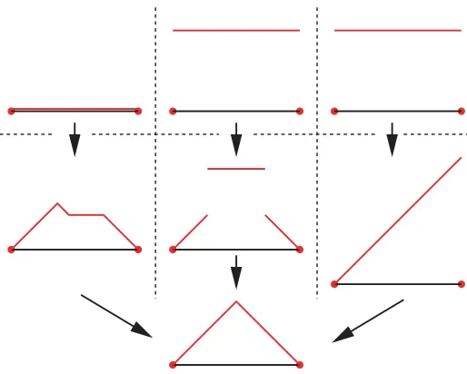
Fig. 1. Schematic representation of the update process for Gauss–Jacobi (left), FM (center), and FS (right) for a one-dimensional eikonal equation with homogenous boundary conditions.
for =1 to N solve f(Uk
1, . . . ,Uk−1,U k
,U
k−1
+1, . . . ,U k−1
N ) =0 for Uk end
end
The update process for the above three methods is schematically represented in Figure 1. Also, as a result of the absence of a true ordering process (only the way arrays are accessed changes), the complexity of the above algorithm can be shown to be of orderN [19], as opposed toNlog2N for FM. However, whether this translates into a computational advantage depends on the geometry of the problem; see section 5. Unlike what is proposed in [16, 19], we consider FS as a direct method for two reasons. First, as shown in section 4, the algorithm has to be run to its completion. Second, the following result gives a natural stopping criterion.
Lemma 3.1. Let Uk, k= 0, . . . ,∞, be the iterates generated by the FS method applied to(1.1), (1.2). Then there exists ¯ksuch that Uk =U¯k for all k≥¯k.
Proof. Consider an arbitrary node i at which the solution has been computed. There exists a path made of successive upwind neighbors fromito Γ. By construction, each successive sweep determines the final value of at least one node on that path, starting on Γ and moving successively toi. This clearly leads to a finite algorithm. The numerical solution at nodeidepends only on the values at its neighbors. If those values do not change at step ¯k+ 1, thenUk
i =U ¯ k
i fork≥¯k.
Essentially, the three methods differ in the order in which the nodes are com-puted. Gauss–Jacobi takes no particular order, FM uses an ordering based on partial numerical solutions, while FS uses a mesh-based ordering. As described above, FS makes full use of the Cartesian structure of the mesh.
For future reference, we now introduce three specific test problems used in this paper. In all three cases, we consider (1.1), (1.2) with Ω = (0,6)2, Γ = (0,0).
Example1. F(x, y) =Cfor all (x, y)∈Ω, no obstacle.1 Example2.
F(x, y) = ∞ if (x−3)
2+ (y−3)2<= 1,
C otherwise,
circular obstacle. Example3.
F(x, y) = ∞ if (x, y)∈Ξ,
C otherwise,
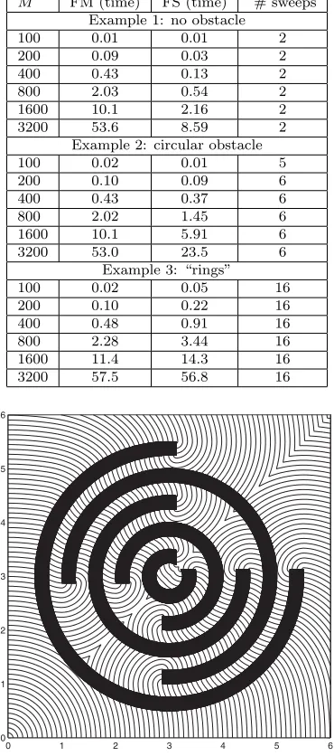
where Ξ is the “rings” of Figure 7.
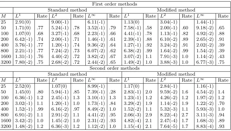
If no local adaption is made when treating problems with obstacles such as Ex-amples 2 and 3, accuracy is lost. Taking, for instance, Example 2, a straightforward discretization would consist of applying any of the above three methodsoutside the circular obstacle using a simple Cartesian mesh. The left half of Table 1 illustrates the loss accuracy incurred by the first and second order FM methods, respectively, i.e., using (2.3) and (2.4).
Table 1
Convergence study for formally first and second order methods in the presence of a circular obstacle (Example 2); M measures the number of nodes on one edge ofΩ, i.e., total number of nodesN=O(M2).
First order methods
Standard method Modified method
M L1 Rate L2 Rate L∞ Rate L1 Rate L2 Rate L∞ Rate
25 2.91(0) 9.00(-1) 6.11(-1) 1.13(0) 3.04(-1) 1.44(-1) 50 1.71(0) .77 5.24(-1) .78 3.52(-1) .79 7.58(-1) .58 2.00(-1) .60 9.18(-2) .65 100 1.07(0) .68 3.27(-1) .68 2.23(-1) .66 4.41(-1) .78 1.13(-1) .82 4.92(-2) .88 200 6.42(-1) .74 2.00(-1) .71 1.46(-1) .61 2.39(-1) .88 6.10(-2) .89 2.65(-2) .91 400 3.76(-1) .77 1.20(-1) .74 9.36(-2) .64 1.27(-1) .92 3.24(-2) .91 2.02(-2) .39 800 2.21(-1) .77 7.24(-2) .73 6.07(-2) .62 6.38(-2) .99 1.64(-2) .99 1.54(-2) .39 1600 1.31(-1) .76 4.40(-2) .72 3.82(-2) .67 3.07(-2) 1.1 7.91(-3) 1.0 1.14(-2) .43 3200 7.80(-2) .75 2.68(-2) .72 2.44(-2) .65 1.49(-2) 1.0 3.88(-3) 1.0 6.77(-3) .75
Second order methods
Standard method Modified method
M L1 Rate L2 Rate L∞ Rate L1 Rate L2 Rate L∞ Rate
25 2.52(0) 1.07(0) 8.99(-1) 1.17(0) 2.84(-1) 1.16(-1)
50 1.45(0) .80 5.94(-1) .85 7.39(-1) .28 2.83(-1) 2.0 9.59(-2) 1.6 4.54(-2) 1.4 100 6.36(-1) 1.2 2.45(-1) 1.3 3.10(-1) 1.3 1.23(-1) 1.2 4.26(-2) 1.2 1.97(-2) 1.2 200 3.02(-1) 1.1 1.20(-1) 1.0 1.73(-1) .84 3.29(-2) 1.9 1.14(-2) 1.9 1.22(-2) .70 400 1.52(-1) .99 6.16(-2) .97 8.49(-2) 1.0 1.52(-2) 1.1 5.32(-3) 1.1 5.93(-3) 1.0 800 6.91(-2) 1.1 2.91(-2) 1.1 4.41(-2) .95 2.06(-3) 2.9 8.22(-4) 2.7 3.11(-3) .94 1600 3.42(-2) 1.0 1.45(-2) 1.0 2.31(-2) .93 4.82(-4) 2.1 2.47(-4) 1.7 1.68(-3) .89 3200 1.48(-2) 1.2 6.36(-3) 1.2 1.12(-2) 1.0 1.15(-4) 2.1 7.64(-5) 1.7 8.83(-4) .93
As can be seen from those results, the standard first order method converges with an average order of only about .75 (in theL1norm) while the standard formally second order method loses a full order (the average rate in theL1norm is about 1.0).
Fig. 2.Mesh structure around the obstacle.
The results in theL2norm are comparable, while theL∞rates are significantly lower. This is not surprising since the underlying solution presents a “shock” at the back of the obstacle (discontinuity of the first derivatives).
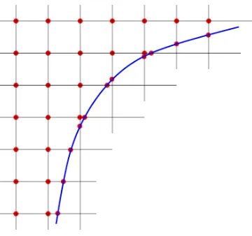
In [2], we started the study of a generalization of the FM method from [14, 15] to problems with obstacles. The nodes are defined on a uniform Cartesian mesh away from the obstacle. Near the obstacle, additional nodes corresponding to the intersection of the obstacle’s boundary with the mesh lines are added; see Figure 2. The detailed solving process is as follows for the modified FM algorithm.
LetX0be a node to be updated. LetX1andX2be a pair of primary neighbors of
X0. Following [15], an upwinding criterion is considered: the characteristic direction should point into the simplex defined by X0, X1, and X2. This is equivalent to requiring the approximate gradient defined by (2.5) to have positive components when expressed in terms of the unit vectors N1 = |XX0−0−XX11| and N2 = |XX0−0−XX22|. In other words,
(N Nt)−1DU >0.
(4.1)
The valueU0atX0 is then determined as follows:
U0= min
⎧ ⎨ ⎩
solution of (2.6) with second order stencil (2.4) if (4.1) is true, solution of (2.6) with first order stencil (2.3) if (4.1) is true, mini=1,2{Ui+|X0−Xi|F(X0)}.
(4.2)
Regardless of the choice of stencil (first or second order), (2.6) has two real solutions, from which we always consider the larger one only, to be consistent with causality. In the first two cases, the values of the partial derivatives of U at X0 are updated using∇U =N−1DU. In the third case, we set ∇U =N
iF(X0), where iis the index corresponding to the case of lowest value forU0. This process is repeated for all pairs of primary neighborsX1andX2, and the lowest resulting value ofU0is kept.
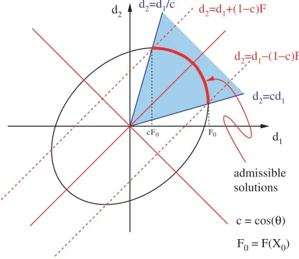
As checking (4.1) accounts for a sizable part of the runtime, the following result is useful in practice.
Lemma 4.1. Let θ, 0 < θ < π, be the angle between N1 and N2. The upwind condition(4.1)is equivalent to
Proof. The result is easy to verify geometrically. Settingdi =DiU, i= 1,2, the scheme (2.6) takes the form
d21−2 cosθ d1d2+d22= sin 2θ F(X
0)2.
This defines an ellipse in the d1d2-plane with major (respectively, minor) semiaxis of length √sinθ
1−cosθF(X0) (respectively, sinθ √
1+cosθF(X0)) in the direction [1,1] (respec-tively, [1,−1]). The upwind condition (4.1) reads as
d1−cosθ d2>0 andd2−cosθ d1>0.
As Figure 3 and a little algebra show, the portion of the ellipse that satisfies the above conditions can also be characterized by|d1−d2|<(1−cosθ)F(X0). Note that this last condition also admits a set of solutions opposite the desired ones on the ellipse depicted in Figure 3. Those solutions are, however, never encountered in practice since only the largest of the two roots of the quadratic equation is retained.
d1 d2=d1+(1−c)F
d2=d1−(1−c)F d2 d2=d1/c
d2=cd1
admissible solutions
c = cos(θ)
F0 = F(X0)
F0 cF0
Fig. 3.Upwind condition; see Lemma4.1and its proof.
For general meshes, the above condition requires the calculation ofU0and has to be checked a posteriori. For a uniform Cartesian mesh of size Δx, (4.3) reads as
|U1−U2|<Δx F(X0)
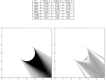
and can be checked a priori, i.e.,withouthaving to solve the quadratic equation (2.6). This explains the large discrepancies in runtimes in favor of the low accuracy method on uniform Cartesian grids reported in Table 2 (see Figure 5 for a comparison of runtime versus accuracy).
mesh-Table 2
Runtimes illustrating the overhead due to higher accuracy for the FM method applied to Example
2; see text for full details.
M Time 1 Time 2 Time 3
100 0.02 0.57 0.60
200 0.10 2.20 2.38
400 0.43 8.93 9.45
800 2.02 34.5 38.1
1600 10.1 143 154
3200 53.0 610 654
Fig. 4. Error propagation downstream of the obstacle for the standard (left) and modified (right) second order FM method (Example2,M = 1600,N =O(M2)). The source is located at (0,0).
independent domain around the source and initializing the values at the nodes there to the corresponding values of the exact solution. This fix was applied to all methods under study here. As illustrated in Table 1, the modified scheme is found to preserve first and second order accuracy in the L1 norm even in the presence of obstacles. For the second order version, theL2 rates of convergence are slightly below 2, while the method appears to converge with order 1 in the maximum norm. In all cases and all norms, the modified method exhibits much better accuracy than the standard method. Error propagation downstream from the obstacle is illustrated in Figure 4 for both standard and modified methods.
It should be noted that second order convergence for the finer meshes was obtained only after rewriting the quadratic formula for solving (2.6) in a form that limits cancellation effects. (Standard IEC559 double precision was used throughout.)
Higher accuracy does not come for free. In Table 2, the overhead corresponding to maintaining optimal accuracy is described in terms of computational time and number of operations.
10–2 10–1 100 101 102 103 10–4
10–3 10–2 10–1 100 101
Runtime
L
1 error
Standard 1st order Modified 1st order Modified 2nd order
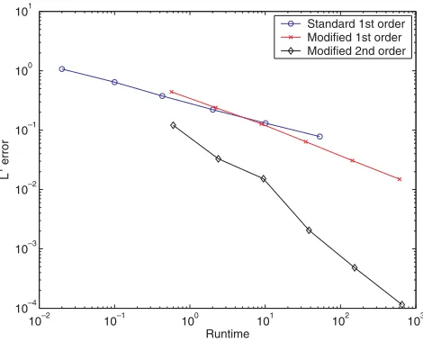
Fig. 5.L1 error versus runtime for the standard “first” order method, the modifed first order method, and the modified second order method applied to Example2.
of the quadratic equation (2.6) and of the upwinding condition (see remarks above). The results for the fully first and second order methods correspond, respectively, to Time 2 and Time 3. The fully second order method is found to be only marginally slower than the fully first order one. It is clear from Table 2 that a significant price has to be paid for the increase in accuracy. However, Figure 5 shows that the advantage in speed for the standard first order is offset by its relative lack of accuracy and slow convergence as the mesh is refined.
FS as described in [16, 19], for instance, is proposed as an iterative method, i.e., the algorithm is stopped before completion according to a stopping criterion of the typeuk+1−ukL1 < δ= 10−10. Figure 6 illustrates the convergence history of the numerical solution toward the exact solution of thediscretizedproblem for Example 3. The discrepancy falls down to zero if one additional step is taken. It is observed that stopping on small decreases, as suggested by the previous criterion, is not advisable. Therefore, running FS until completion appears to be the best strategy, and the algorithm has to be considered as a “direct” method.
For both FM and FS, obstacles can be implemented as domains with truly infinite speed (in which case, no calculations are made at nodes inside the obstacle), or a sufficiently large but finite slowness can be assigned to nodes inside the obstacle and the solution can be computed there. Our implementation uses the former approach. As can be expected and is illustrated in Figure 6, those choices do not affect the solutions of the discretized problems.
2 4 6 8 10 12 14 10–10
10–5 100 105
number of sweeps
distance to final iterate L1 (finite slowness) L∞ (finite slowness) L1
L∞
Fig. 6.L1andL∞norms of the difference between the exact solution of thediscretizedproblem with the FS method and iterates after each sweep; rings (Example3);M = 1600. The curves with “finite slowness” are obtained by treating the obstacle as a domain with large slowness; the other curves correspond to a genuine obstacle (slowness =∞).
both methods perform in a way very similar to Example 2, with a slight advantage for FS, while on Example 3 FM is faster for all but the finest mesh.2
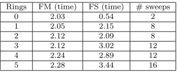
The results from Table 3 also show that, for moderate mesh sizes, the more com-plicated the domain is, the better FM performs with respect to FS. Indeed, while FM continually advances the wavefront, FS has to do another set of sweeps every time the direction of propagation changes. In the case of Example 3, for instance, that direction changes several times; see Figure 7. In Table 4, the runtimes for a modified Example 3 are reported: the number of partial rings was increased from zero to a total of five as displayed in Figure 7. It is observed that the runtime is roughly constant for FM as the complexity of the domain (number of rings) increases. For FS, however, the runtime increases, although in a nonuniform way. This nonuniformity results from both the geometry of the domain (odd/even number of rings) and our specific implementation.
As argued in [19], FS has an asymptotic computational complexity ofO(N) while FM’s isO(Nlog2N). Eventually, FS overcomes FM, even for nontrivial examples such as Example 3, as the mesh gets fine enough. The constants of proportionality involved in those asymptotic relations are not easy to analyze. For specific examples, those con-stants can be estimated numerically. Assuming runtimes for FS and FM to be, respec-tively, equal toCF SmN andCF MNlog2N, wheremis the number of sweeps required by FS, one can use results similar to those from Table 3 to roughly determine the two constantsCF S andCF M. An empirical condition under which FS is faster than FM can then be derived. Using best fits to the above examples and cases, one finds here
m.6 log2N.
Table 3
Runtime for first order FM and FS on a uniform Cartesian mesh for Examples 1,2, and3
(N=O(M2)).
M FM (time) FS (time) # sweeps Example 1: no obstacle
100 0.01 0.01 2
200 0.09 0.03 2
400 0.43 0.13 2
800 2.03 0.54 2
1600 10.1 2.16 2
3200 53.6 8.59 2
Example 2: circular obstacle
100 0.02 0.01 5
200 0.10 0.09 6
400 0.43 0.37 6
800 2.02 1.45 6
1600 10.1 5.91 6
3200 53.0 23.5 6
Example 3: “rings”
100 0.02 0.05 16
200 0.10 0.22 16
400 0.48 0.91 16
800 2.28 3.44 16
1600 11.4 14.3 16
3200 57.5 56.8 16
0 1 2 3 4 5 6
0 1 2 3 4 5 6
Fig. 7.Propagation around an obstacle: Example3, FM withM= 800. The source is located at(0,0).
In other words, for a “reasonable” 800×800 mesh (N = 8002), FS will be faster than FM as long as the number of sweeps necessary for convergence does not exceed about 11. This is in good agreement with Table 4.
Table 4
Runtime and operation count with differing numbers of concentric partial rings (M= 800).
Rings FM (time) FS (time) # sweeps
0 2.03 0.54 2
1 2.05 2.15 8
2 2.12 2.09 8
3 2.12 3.02 12
4 2.24 2.89 12
5 2.28 3.44 16
much less flexible. Second, the examples considered show that both methods should be thought of as direct and not iterative algorithms. This is obvious for FM. For FS, a natural stopping criterion is proposed and justified. Finally, FS and FM have asymptotic orders of complexity of, respectively,O(mN) andO(Nlog2N), wherem
is the number of sweeps andN is the total number of nodes. On a realistic grid, FS will be faster than FM for problems with simple geometry. For strongly nonuniform problems and/or complex geometry, the situation may be reversed.
Both methods can be relatively easily extended to more general convex Hamil-tonians [15, 16]. Behaviors similar to those reported here are expected. The case of nonconvex Hamiltonians is more complex, even with respect to the construction of appropriate numerical fluxes. Very few schemes have been proposed (see, for instance, [8], where a Lax–Friedrichs sweeping method is introduced); more needs to be done to develop fast and accurate methods for those problems.
Acknowledgments. The authors are grateful to Hongkai Zhao for his helpful comments and to the referees for remarks that led to a better presentation of the results.
REFERENCES
[1] R. Abgrall,Numerical discretization of the first order Hamilton-Jacobi equations on trian-gular meshes, Comm. Pure Appl. Math., 49 (1996), pp. 1339–1377.
[2] S.A. Ahmed, R. Buckingham, P.A. Gremaud, C.D. Hauck, C.M. Kuster, M. Prodanovic, T.A. Royal, and V. Silantyev,Volume determination for bulk materials in bunkers,
Internat. J. Numer. Methods Engrg., 61 (2004), pp. 2239–2249. [3] J. Bentley,Thanks, heaps, Comm. ACM, 28 (1985), pp. 245–250.
[4] M. Bou´e and P. Dupuis, Markov chain approximations for deterministic control problems with affine dynamics and quadratic cost in the control, SIAM J. Numer. Anal., 36 (1999), pp. 667–695.
[5] M. Crandall, L. Evans, and P.-L. Lions,Some properties of viscosity solutions of Hamilton-Jacobi equations, Trans. Amer. Math. Soc., 282 (1984), pp, 487–502.
[6] M. Crandall and P.-L. Lions,Two approximations of solutions of Hamilton-Jacobi equations,
Math. Comp., 43 (1984), pp. 1–19.
[7] C. Hu and C.-W. Shu,A discontinuous Galerkin method for Hamilton–Jacobi equations, SIAM
J. Sci. Comput., 21 (1999), pp. 666–690.
[8] C.-Y. Kao, S. Osher, and J. Qian,Lax-Friedrichs sweeping scheme for static Hamilton-Jacobi equations, J. Comput. Phys., 196 (2004), pp. 367–391.
[9] G. Kossioris, C. Makridakis, and P. Souganidis, Finite volume schemes for Hamilton-Jacobi equations, Numer. Math., 83 (1999), pp. 427–442.
[10] S. Osher and C.-W. Shu,High-order essentially nonoscillatory schemes for Hamilton–Jacobi equations, SIAM J. Numer. Anal., 28 (1991), pp. 907–922.
[11] J. Qian and W.W. Symes,An adaptive finite difference method for traveltimes and amplitudes,
Geophysics, 67 (2002), pp. 167–176.
[12] E. Rouy and A. Tourin, A viscosity solutions approach to shape-from-shading, SIAM J.
[13] J.A. Sethian,Fast marching methods, SIAM Rev., 41 (1999), pp. 199–235.
[14] J.A. Sethian and A. Vladimirsky,Fast methods for the Eikonal and related Hamilton-Jacobi equations on unstructured meshes, Proc. Natl. Acad. Sci. USA, 97 (2000), pp. 5699–5703. [15] J.A. Sethian and A. Vladimirsky,Ordered upwind methods for static Hamilton–Jacobi
equa-tions: Theory and algorithms, SIAM J. Numer. Anal., 41 (2003), pp. 325–363.
[16] Y.H.R. Tsai, L.T. Cheng, S. Osher, and H.K. Zhao,Fast sweeping algorithms for a class of Hamilton–Jacobi problems, SIAM J. Numer. Anal., 41 (2003), pp. 673–694.
[17] J.N. Tsitsiklis,Efficient algorithms for globally optimal trajectories, IEEE Trans. Automat.
Control, 40 (1995), pp. 1528–1538.
[18] J.W.J Williams,Heapsort, Comm. ACM, 7 (1964), pp. 347–348.