ENHANCED ADVANCING FRONT TECHNIQUES FOR MESH GENERATION IN RADIATIVE HEAT TRANSFER PROBLEM
ZURAIDA ABAL ABAS
ENHANCED ADVANCING FRONT TECHNIQUES FOR MESH GENERATION IN RADIATIVE HEAT TRANSFER PROBLEM
ZURAIDA BINTI ABAL ABAS
A thesis submitted in fulfilment
of the requirements for the award of the degree of Doctor of Philosophy (Mathematics)
Faculty of Science Universiti Teknologi Malaysia
ACKNOWLEDGEMENT
So many people have played a significant role in my life as I entered the world of PhD student. I would like to thank my supervisor, Prof Dr. Shaharuddin Salleh who has always provided ideas, guidance and motivation as well as his assistance throughout this work. Special thanks to my other supervisor, Prof Dr. Zainuddin Abd Manan who introduced me the concept of ethylene furnace.
I also would like to thank the staff of Unit Cuti Belajar as well as Universiti Teknikal Malaysia Melaka and Kementerian Pengajian Tinggi for providing support and financial assistance during my study. Special thanks to Prof Dr Shahrin Sahib for his support and Dr. Simon Botley for providing language assistance. Same thing goes to all my friends who have always shared the up and down of PhD study.
ABSTRACT
ABSTRAK
TABLE OF CONTENTS
CHAPTER TITLE PAGE
TITLE PAGE i
DECLARATION ii
DEDICATION iii
ACKNOWLEDGEMENT iv
ABSTRACT v
ABSTRAK vi
TABLE OF CONTENTS vii
LIST OF TABLES xi
LIST OF FIGURES xiii
LIST OF SYMBOLS / NOTATIONS xxvi
1 INTRODUCTION 1.1 Research Background 1
1.2 Problem Statement 3
1.3 Objective and Scope of the Research 4
1.4 Research Methodology 5
1.5 Significance of the Research 9
Process 14 2.3 The Phenomena of Heat Transfer in
Ethylene Furnace and the Current Technique
of Monitoring Heat Transfer Parameter 18
2.4 Mesh Triangulation 19
2.5 The General Basic Step of the Standard
Advancing Front Technique (SAFT) 21 2.6 Recent Approaches in Advancing Front
Technique 25
2.7 Mesh Quality Improvement 31
2.8 The Concept of Radiation 33
2.9 The Discrete Ordinate Method (DOM) 35 2.10 The Sensor for High Temperature 37
3 THE ENHANCED ADVANCING FRONT
TECHNIQUE -1
3.1 Introduction 40
3.2 The Condition of Invalid or Undecided Element
Creation 41
3.3 The Extension of a Normal Case in the SAFT for
Triangular Element Creation 43
3.4 The Implementation of Element Creation Procedure Based on Five Cases of EAFT-1 in AutoCAD LT 48 3.5 The Mathematical Equations Behind the Work of
EAFT-1 in AutoCAD 66
3.6 The Significance of Incorporating Extension Cases to the Standard Algorithm of the
Advancing Front Technique 68
3.7 The Simulation Results 68
4 THE ENHANCED ADVANCING FRONT
TECHNIQUE-2
4.2 The Problem Statement and the Simplified
Version of the Conceptual Model 79 4.3 The Enhanced Advancing Front Technique-2
(EAFT-2) Algorithm 81
4.3.1 The Layer Concept and its Significance to
the EAFT-2 83
4.3.2 The General Idea of the Enhanced
Advancing Front Technique-2 (EAFT-2) 85 4.3.3 The Six Cases of Consideration for
Element Creation Procedure 87 4.3.4 The Implementation of Element Creation
Procedure Based on Six Cases of EAFT-2
In AutoCAD LT 92
4.3.5 The Mathematical Equations Behind the
Work of EAFT-2 in AutoCAD 108 4.3.6 The Entire Front Starting with the
Shortest Edge as the Departure Zone 108 4.3.5 The Significance of EAFT-2 115 4.4 The Integration of the Value from the Sensors
and the Unstructured Mesh with the Governing
Equation of Radiative Heat Transfer 116 4.5 The difference between SAFT and EAFT-2 117 4.6 The Simulation Result 118
5 THE ENHANCED ADVANCING FRONT
TECHNIQUE-3
5.1 Introduction 129
5.2 The Conceptual Model 130 5.3 The Enhanced Advancing Front Technique-3
Algorithm 131
5.3.1 The General Idea of the Enhanced
Element Creation Procedure 135
5.3.3 The Implementation of Element Creation Procedure Based on Seven Cases of EAFT-3 In AutoCAD LT 140
5.3.4 The Mathematical Equations Behind the Work of EAFT-3 in AutoCAD 162
5.3.5 The Departure Zone in EAFT-3 for the Element Creation Procedure 163
5.3.6 The Newly Created Post-processing Procedure 170
5.3.5 The Significance of EAFT-3 171
5.4 The Difference Between SAFT and EAFT-3 172
5.5 The Simulation Result 173
6 CONCLUSION 185
REFERENCES 190
LIST OF TABLES
TABLE NO. TITLE PAGE
2.1 The configuration of ethylene furnace taken from [33] 15 3.1 The relationship between QEAS and mesh quality together with
the total elements in the range respectively for initial
unstructured grids generated with EAFT-1 for the domain as in Figure 3.15.
71
3.2 The relationship between QEVS and mesh quality together with the total elements in the range respectively for unstructured grids generated with EAFT-1 for the domain as in Figure 3.15
73
3.3 The relationship between QEAS and mesh quality together with
the total elements in the range respectively for unstructured grids generated with EAFT-1 for the domain as in Figure 3.18
75
3.4 The relationship between QEVS and mesh quality together with
the total elements in the range respectively for unstructured grids generated with EAFT-1 for the domain as in Figure 3.18
76
4.1 The result for the layer concept for Figure 4.3b 84 4.2 The relationship between QEAS and mesh quality together with
the total elements in the range respectively for unstructured grids generated with EAFT-2 for the domain of one circle as in Figure 4.19
122
4.3 The relationship between QEASand mesh quality together with the total elements in the range respectively for unstructured grids generated with EAFT-2 for the domain of two circles as
in Figure 4.21 124
5.1 The number of elements in percentages with respect to the range of the quality of the initial unstructured mesh generated
5.2 The number of elements in percentages with respect to the range of the quality of the initial unstructured mesh generated with SAFT in GAMBIT for the conceptual model of ethylene
furnace 178
5.3 The number of elements in percentages with respect to the range of the quality of the final unstructured mesh generated
with EAFT-3 for the conceptual model of ethylene furnace 180 5.4 The mesh quality of initial unstructured mesh for the simplified
conceptual model with one circle by using algorithm of
LIST OF FIGURES
FIGURE NO.
TITLE PAGE
1.1a The framework of the research – part 1 8
1.1b The framework of the research – part 2 9
2.1 The ethylene furnace plant taken from [49] 14
2.2 The illustration of radiant section or firebox in ethylene furnace
taken from [33] 15
2.3 The interaction of the processes in the ethylene furnace 17 2.4a Elements that satisfy the circumcircle property. 20 2.4b Elements that do not satisfy the circumcircle property. 20 2.5a Detection of the elements which contain the new inserted point. 20 2.5b The creation of new elements by connecting the new point to the
points at the boundary of the convex cavity.
20
2.6 The illustration for the incremental point insertion strategy. 21 2.7a A two dimensional domain with connected boundary curves 22 2.7b A set of edges forming initial front and the background grid
consists of triangle ABC and ADC 22
2.8 The illustration of element with regards to front, taken from [68] 23 2.9a The selected edge
a,b and the position of IP 23 2.9b A circle is constructed with centre at IP and the radius of thecircle following the empirical rule 23
2.10 The illustration of the front ‘marching’ process into the interior of
2.11 The general scheme of SAFT 25 2.12 The determination of optimal number of points taken from [75] 26 2.13 The first local umbrella at the left and the extremely right is
completing two local umbrella [76] 27
2.14 Choosing the correct segment at point p[76] 27 2.15a The first element is generated by connecting the centre of the
circle and become the initial front, taken from [77] 28 2.15b The second element is generated by adding a new circle and
connect the centre of the circle to the existing element, taken
from [77] 28
2.16a The packing of circles with random size across the domain, taken
from [77] 28
2.16b The resulted unstructured mesh with random size, taken from [77] 28 2.17 The mesh/grid generation algorithm taken from [78] 29 2.18 The latest approach and advancement for advancing front
technique in terms of element construction 30
2.19 Diagonal swapping 32
2.20 The shift for the interior node 32
2.21 The radiative heat transfer in Cartesian coordinate system taken
from [88] 34
2.22 Cell centred control volume in 2D unstructured mesh, taken from
[88] 36
2.23 A thermocouple made from iron and constantan wire taken from [90]
38
2.24 A typical RTD sensor taken from [95] 38
2.25 A variety of sizes and shapes of thermistors taken from [97] 39 3.1a Definition of boundary edges at boundary curves 42 3.1b Edge
7 9, as the base edge. The IP is out of the boundary and no3.2 The second problem where the base edge is (a,b) and it cannot
connect to the IP directly 42
3.3a No objects lie within the circle 44
3.3b An equilateral triangle is constructed 44
3.4a Two types of object lie within the circle which are active nodes
and edges 45
3.4b Node d is selected as the vertex 45
3.5a An active edge intersected with the circle and Lp p1 2 r 46 3.5b The IP becomes the new active node d for the triangular element 46 3.6a The intersected active edge is
b,c and1 2
p p
L r 47
3.6b The triangular element is constructed by connecting the node
associated with the intersected active edge with the base edge 47
3.7 The general scheme of EAFT-1 47
3.8 The object snap mode in drafting setting 48
3.9a The computational domain 49
3.9b The background mesh consists of triangle ABD and BCD 49 3.9c A set of nodes are placed by using command multiple points 50 3.9d The crosshair is positioned at the initial node until the small
purple color circle appears at the node
51
3.9e The crosshair is moved towards the end node until the small purple colored circle appears at the respective node
51
3.9f The line which represents boundary edge is automatically created where it connects the initial node and end node
52
3.9g A set of boundary edges 52
3.10a Active edge considered for example 1 is
a,b 543.10b The selection of circle drawing tool 54
3.10c The crosshair is moved towards node b until a small purple
3.10d A circle with its centre at node a and radius equal to the length of
the active edge is created 55
3.10e A circle with its centre at node b and radius equal to the length of
the active edge is created 56
3.10f A command to create single point is selected 56 3.10g The crosshair is moved towards the point where the circles
intersect until small purple colored x appear at the intersection 57 3.10h The intersection of the two circles is selected as the IP and the
previous two circles are deleted 57
3.10i A circle for example 1 with its centre at IP and radius obtained
from empirical rule 58
3.10j An equilateral triangle is constructed for example 1 59 3.11a Active edge considered for example 2 is
a,b and a circle isconstructed for example 2 60
3.11b Node c is selected as a vertex for example 2 61 3.12a Active edge considered for example 3 is
a,b and a circle isconstructed 62
3.12b Intersection points marked as point p1and p2 63 3.12c Node c is selected to be the vertex to form the triangle element
for example 3 63
3.13a Active edge considered for example 5 is
a,b and a circle isconstructed 64
3.13b The intersection points p1 and p2and its distance 65 3.13c Equilateral triangle is created when IP is selected and becomes
node e for example 4 66
3.14a A domain with background grid consists of triangle ABD and
ADC 68
3.14b A set of boundary edges 68
3.15 The resulted initial unstructured triangular mesh using EAFT-1 69
3.16b Element with quality 0QEAS 0 25. 70 3.16c Element with quality 0 25. QEAS 0 5. 71 3.16d Element with quality 0 5. QEAS 0 75. 71
3.17a Element with quality QEVS 0 72
3.17b Element with quality 0QEVS 0 25. 72
3.17c Element with quality 0 25. QEVS 0 5. 72 3.17d Element with quality 0 5. QEVS 0 75. 72 3.18 The resulting unstructured mesh at the end of mesh smoothing
procedure 74
3.19a Element with quality QEAS 0 74
3.19b Element with quality 0QEAS 0 25. 74
3.19c Element with quality 0 25. QEAS 0 5. 75
3.20a Element with quality QEVS 0 76
3.20b Element with quality 0QEVS 0 25. 76
3.21 The contour of temperature distibution of the flue gas 77
3.22 The plot of convergence for the simulation 77
4.1a A simplified problem domain for the initial study with only 1
circle representing half a reactor coil 80
4.1b A simplified problem domain for the initial study with two circles
representing 1 complete reactor coil 80
4.2a Definition of boundary edges at boundary curves 82 4.2b The whole domain is divided into sub-regions 83 4.3a A straight line AB before applying layer concept 84 4.3b A set of nodes are placed at the line segments produced by
4.4 Applying the layer concept at the newly created line segment (the
newly created boundary of the sub-regions- AB, CD, EF and GH) 85 4.5a
11 12,
is selected as the base edge for element construction 86 4.5b A triangular element is constructed with
11 12,
as the base edge 86 4.6a Intersection point of the circle is the IP. Base edge is
a,b 86 4.6b IP on the perpendicular bisector of the base edge 864.6c A circle is constructed with IP as centre 87
4.6d A triangular element is constructed by having IP as the vertex 87
4.7a No object lies within the circle 88
4.7b An equilateral triangle is constructed 88
4.8a Two types of the object lie within the circle which are active
nodes and active edges 89
4.8b Node d is selected as the vertex 89
4.9a An active edge intersected with the circle with 1
bp
L r 90
4.9b The IP becomes node d , the new active node for the triangular
element 90
4.10a The intersected active edge is
b,c with Lbp1r 91 4.10b The triangular element is constructed by connecting the nodeassociated with the intersected active edge to the base edge 91 4.11a Two active edges with equal length to the radius intersected with
the circle and at the same time all the nodes of the active edges
are at the circum circle 92
4.11b Three equilateral triangle elements are constructed simultaneously 92 4.12a The base edge considered is
a,b and its IP for example 1 93 4.12b Position the crosshair until a small purple colored circle appearsat IP 94
4.12c The crosshair is moved towards either node of the base edge until
4.12d A circle with its centre at IP and rLbase _ edge is automatically
created 95
4.12e An equilateral triangle is constructed for example 1 96 4.13a A circle with its centre at IP and rLbase _ edge is constructed for
example 2 97
4.13b Among the process to creating the temporary line from node d to
IP 98
4.13c The distance between node d and IP is 0.2604 99 4.13d The distance between node c and IP is 0.5049 99 4.13e Node dis selected as a vertex for example 2 100 4.14a A circle with its centre at IP and rLbase _ edge is constructed for
example 4 101
4.14b Creating the intersection point 1p 102
4.14c A temporary line to determine the distance Lbp1 102 4.14d An equilateral triangle is created when IP is selected as the vertex
for example 4 103
4.15a A circle with its centre at IP and rLbase _ edge is constructed for
example 5 104
4.15b A temporary line to determine the distance Lbp1 105 4.15c Node c is selected to be the vertex of the new triangular element
for example 5 105
4.16a A circle with its centre at IP and rLbase _ edge is constructed for
example 6 106
4.16b One of the new edges that need to be created by connecting node
e to the node that lie at the circum circle 107 4.16c Three equilateral triangles are constructed for example 6 107
4.17a The initial front 111
4.17c The second triangular element creation in the front 111 4.17d The third triangular element creation in the front 111 4.17e The entire active edges of the first or initial front has been
completely triangulated and form the second front 112 4.17f The entire active edges of the second front has been completely
triangulated and form the third front 112
4.17g The entire active edge of the third front has been triangulated 113
4.17h Triangular element mesh in the sub-region 113
4.18 EAFT-2 without the layer concept for domains with one circle 120 4.19 EAFT-2 incorporating the layer concept for domains with one
circle 120
4.20a Element with quality QEAS 0 121
4.20b Element with quality 0QEAS 0 25. 121
4.20c Element with quality 0 25. QEAS 0 5. 122 4.20d Element with quality 0 5. QEAS 0 75. 122 4.21 EAFT-2 incorporating the layer concept for domains with two
circles representing one complete reactor coil 123
4.22a Element with quality QEAS 0 124
4.22b Element with quality 0 25. QEAS 0 5. 124 4.22c Element with quality 0 5. QEAS 0 75. 124 4.23 The plot of convergence for simplified conceptual model with one
circle 125
4.24 The plot of convergence for simplified conceptual model with two
circle 126
4.25 The contour of temperature (K) distibution of the flue gas for the
domain with 1 circle 127
4.26 The contour of temperature (K) distibution of the flue gas for the
4.27 The flue gas temperature (K) profile along the width of the
furnace with one circle at y=1.5 128
4.28 The flue gas temperature (K) profile along the width of the
furnace with two circles (one complete reactor coil) at y=1.5 128 5.1 The top view of the furnace taken from [33] with sensors placed
along the wall 131
5.2a Definition of boundary edges at boundary curves 132 5.2b The whole domain is divided into sub-regions 132 5.3 Applying the layer concept at the newly created line segment (the
newly created boundary of the sub-regions - AB and BC) 133 5.4a The base edge is
11 12,
. Intersection point of the two circles isthe IP 134
5.4b IP on the perpendicular bisector of the base edge 134
5.4c A circle is constructed with IP as centre 135
5.4d A triangular element is constructed by having IP as the node 135
5.5a No object lies within the circle 136
5.5b An equilateral triangle is constructed 136
5.6a Two types of the object lie within the circle which are active
nodes and active edges 136
5.6b Triangular element is constructed with edge
b,d 1365.7a An active edge intersected with the circle 137
5.7b The IP becomes the new active node for the triangular element 137 5.8a The intersected active edge is
b,c . The length of intersectionpoint p1and p2with the circle is more than the length of the
radius and at the same timeLie2* Lbase _ edge 138 5.8b The triangular element is constructed by connecting the node
associated with the intersected active edge with the base edge 138 5.9a The intersected active edge is
b,c . The three conditions whichare Lp p1 2 r, L( b,c )2* L( a ,b ) and 0 1 p
( b ,c )
L .
L are satisfied.
5.9b The triangular element is constructed by connecting the node
associated with the intersected active edge to the base edge 139 5.10a The intersected active edge is
b,c . The three conditions,1 2
p p
L r, L( b,c )2* L( a ,b ) and p 0 1
( b ,c )
L .
L are satisfied.
140
5.10b The triangular element is constructed by connecting the node
associated with the intersected active edge to the base edge. 140 5.11a The base edge considered is
a,b and its IP for example 1 141 5.11b The crosshair is first positioned at IP and left click on it when asmall purple colored circle appears at IP 142
5.11c The crosshair is moved towards either of the nodes of the base edge until a small purple colored circle appears at the respective
node 143
5.11d A circle is automatically created 143
5.11e Left click on the circum circle and delete the existed radius value
in the properties window 144
5.11f A circle with its centre at IP and r0 0679. is created 144 5.11g An equilateral triangle is constructed for example 1 145 5.12a A circle with its centre at IP and r0 0549. is constructed
for example 2 146
5.12b The new triangular element is a combination of edge
a,b ,
b,c and
a,c as the three sides of the triangle for example 2 1475.13a A circle with its centre at IP and r0 8. * Lbase _ edge is constructed
for example 3 148
5.13b Edge
b,c intersects with the circle with its length is Lie 0 75. 149 5.13c The intersection points are created and Lp p1 2 r 149 5.13d Node c is selected to be the vertex to form the triangle elementfor example 3 150
5.14b The three edges
b,c ,
b,d and
c,d are connected to themselves and they become the sides of the second triangularelement automatically 151
5.15a The base edge considered is
a,b for example 5 152 5.15b Edge
a,c intersects with the circle with its length is0 7202
ie
L . 153
5.15c The intersection points are created and its distance is Lp p1 2 r 154 5.15d The crosshair is moved towards the intersected active edge until a
small purple colored symbol of perpendicular appears at the
intersected active edge 154
5.15e The perpendicular line of the intersected active edge connecting
to the IP is then created with Lp 0 1451. 155 5.15f The first element is created when the nodes of the base edge are
connected to node d 155
5.15g The second element is created when the node of the active edge of
a,c is connected to node d 1565.16a A circle with its centre at IP and r0 8. * Lbase _ edge is constructed 157 5.16b The intersection points are created and Lp p1 2 r 158 5.16c A triangular element is constructed with edges
a,b ,
a,d and
b,d as the three sides of the triangular element for example 6 1585.17a A circle with its centre at IP and r0 8. * Lbase _ edge is constructed
for example 7 159
5.17b The edge
a,c intersects with the circle with its length is0 5891
ie
L . 160
5.17c The intersection points are created and its distance is Lp p1 2 r 161 5.17d The perpendicular line is created and its length is Lp 0 0537. 161 5.17e Node c which is the node associated with active edge
a,c is5.18a The initial or first front 165 5.18b The first and second triangular element creation in the front 165 5.18c The third and forth triangular element creation in the front 166 5.18d All the active edges of the departure zone group of the initial front
become passive and form the second front 166
5.18e All the active edges of the departure zone group of second front
become passive and form the third front 167
5.18f All the active edges of the departure zone group of the third front
become passive and form the fourth front 167
5.18g All the active edges of the departure zone group of fourth front
become passive and form the fifth front 167
5.18h Triangular element mesh in the sub-region 167
5.19a ABE and BCE are poor elements 170
5.19b Adjacent element is subdivided at the centroid 170 5.19c A new polygon is formed when the poor elements and the newly
developed element which share the same edge with the poor
elements are deleted 171
5.19d New elements are created when the polygon is subdivided at the
centroid 171
5.20 The resulting initial mesh using the algorithm of EAFT-3 for
conceptual model of ethylene furnace 174
5.21a Zoom of the initial unstructured triangular elements at the inlet
reactor 175
5.21b Zoom of the initial unstructured triangular elements at the outer
reactor coils 175
5.22a Element with quality QEAS 0 176
5.22e Element with quality 0 75. QEAS 0 9. 176
5.22f Element with quality 0 9. QEAS 1 176
5.23 The resulting initial unstructured mesh with SAFT algorithm for
conceptual model of furnace 178
5.24 The resulting final mesh for the conceptual model with EAFT-3
after the post-processing procedure 179
5.25a Element with quality QEAS 0 180
5.25b Element with quality 0QEAS 0 25. 180
5.25c Element with quality 0 25. QEAS 0 5. 180 5.25d Element with quality 0 5. QEAS 0 75. 180 5.26 The resulting initial unstructured mesh using the algorithm of
EAFT-3 for the simplified conceptual model as in Figure 4.1a 181
5.27 The plot for convergence 182
5.28 The contour of the flue gas temperature in the furnace 183 5.29a Circumferential heat flux distribution (Wm-2) 184 5.29b Circumferential reactor coil skin temperature (K) 184 6.1 The contribution of the study in the area of unstructured mesh is
shaded with gray color
188
6.2 The comparative progressive between all the versions of the EAFT
LIST OF SYMBOLS / NOTATIONS
Roman Letters
a,b,c,d ,e - nodes considered for element creation procedure A,B,C,D - node forming the background grid
i A
- ith surface area n n 1
b , - distance of the potential point from the edge which join node
nand n 1
c - intersection with y-axis
i
d - layer i
D - the product of the normal unit vector at the ith surface and the
intensity direction m E - emissive power
b
E
- emissive power of blackbody
s
E
- emissive power of real surface
i
Edge _ sensor - sensor boundary edge i - node
idim - dimensionality of the problem domain
IP - ideal point
K - number of pivot point
I - radiation intensity
b
I
- radiation intensity of blackbody
s
I
- radiation intensity of real surface
m
m'
I - intensity along direction m'
i
m P
I
- intensity at cell Pi
l - length of the selected shortest active edge L - total length of the straight line
1
bp
L
- length between the connected node of the base edge and intersection point p1
i
Ld - Length of the layer
base _ edge
L
- length of the base edge
ie
L
- the whole length of the intersected active edge
p
L - the length of the perpendicular line of the intersected active edge connecting directly to the IP
1 2
p p
L
- length between the intersection points
m - number of layer
ie
m - the slope of intersected active edge M - total number of discrete directions
M - number of sub-regions
n - node
n - total number of edges from the layer concept
s
n
- number of nodes adjacent to nodei
n - outward surface normal
i
N - outer boundary nodes
p - centre of local umbrella
p - total number of inner boundary edges in the whole domain
s
p , pe - point at local umbrella
1
p , p2 - intersection points of the active edge and circle
Pi - neighbour cell of cell P with ith surface as the same face
between P and Pi
q - total number of outer boundary edges in the whole domain
EAS
Q - EquiAngle Skew
EVS
Q - EquiSize Skew
r - radius of the circle for triangular element creation
j
r
- reference number for inner boundary edge
k
r
- reference number for outer boundary edge
l
r - reference number for edges from layer concept
t
r - reference number for new edge created in the whole domain
r - position vector
w
r
- position vector for a point on a diffusively emitting and reflecting gray surface
n
N - optimal number of new points P
N
- total surface number for cellP
s
- stretching parameterS - area of the mesh elements
eq
S
- maximum area of the equilateral triangle circumscribing radius of which is identical to that of the mesh element
T - absolute temperature
i
T - temperature obtained from the sensor at outer boundary node
i
TEdge _ sensor - average temperature value of sensor boundary edge
m'
w - solid angle associated with direction m'
j
x
- x coordinate of the neighbouring node with reference number j
j
y
- ycoordinate of the neighbouring node with the reference number j
x ,yc c
- the co-ordinate of active node c
h,k - The co-ordinate of IP
x ,yp1 p1
- the co-ordinate of intersection point p1
x ,yp2 p2
- the co-ordinate of intersection point p2
x ,yp p
- the co-ordinate of the point where both of the perpendicularline and the intersected active edge cross
Greek Letters
n
- angle between edges
- size parameter of the mesh n 1 n,
, n n 1, - length of adjacent edge - orientation of the cells
- Stefan-Boltzmann’s constant
s
- scattering coefficient
- surface emissivity
- absorption coefficient
- extinction coefficient
- direction of intensity
' - scattering phase function from the incoming direction, ' to the outgoing direction,
+
- leaving radiation intensity direction
- - arriving radiation intensity directions
m
- discrete direction of radiation intensity
- cosines of direction along the Cartesian co-ordinate x
- cosines of direction along the Cartesian co-ordinate z
P V
- the volume of cell P
max
- maximum angle between edges
min
- minimum angle between edges
eq
CHAPTER 1
INTRODUCTION
1.1 Research background
Ethylene is the greatest olefin market where most of it is consumed in plastic production [1]. 90% of ethylene in the Europe is produced from steam cracking using naphtha as the feedstocks while in North America and Middle East use ethane and propane as the feedstocks [2]. Ethylene is an important chemical compound produced in the petrochemical industry and is produced from the steam cracking process in ethylene cracker furnaces [3, 4]. In steam cracking, heat is used for breaking or cracking down the saturated hydrocarbon or feedstocks into smaller hydrocarbon in the reactor coils or reactor tubes, which eventually produces the desired products such as ethylene.
The desired parameters of the heat transfer in ethylene furnace study are the temperature and the radiative heat flux. In order to obtain such parameters, the whole process of the fluid flow simulation in Computational Fluid Dynamics (CFD) need to be done where it involves all three elements namely pre-processing, solving and the post-processing. As a matter of fact, structured or unstructured triangular mesh formation fall into the pre-processing element in CFD [14]. The generation of triangular mesh is an important step for approximating solutions to boundary value problems. Among the two type of meshes, unstructured mesh are becoming predominant because of its ability of modeling complex geometry as well as the natural environment it has for adaptivity [15, 16].
There are two basic approaches for unstructured mesh namely the Delaunay triangulation and the advancing front technique. The Delaunay triangulation is a method of generating elements by adding or inserting points in the interior and reconnecting it to form the element [15, 17-21]. The insertion of the points can be controlled by several methods reported in [22]. On the other hand, the advancing front technique generate element with its key algorithmic step is the appropriate introduction of the new elements to the empty region [19, 21, 23]. It must be noted that the elements and the nodes in this technique are placed simultaneously in the region [24].
The advancing front technique places a new element by considering an ideal point generated as well as the existing nodes in the circle constructed. The centre of the circle is the ideal point and the radius is calculated based on the empirical rules for the element creation procedure. The advancing front technique is guaranteed to preserve boundary integrity as well as having the capacity to create triangular elements with high aspect ratios in the boundary-layer region [15, 25]. However, there are also method of combining the approach of Delaunay and advancing front techniques for generating unstructured mesh such as in [25-31].
(1) A new element is created with a new node as a vertex in which the new node is joined to the edge being considered.
(2) An already existing front node satisfying certain conditions in the proximity of the edge being considered is used to create a new element.
(3) Neither of the cases above in which an efficient algorithm of mesh generation should be able to tackle such a problem.
With the advancing front technique as the approach for triangulation in the study, it can be seen that there is an improvement that need to be done towards the algorithm. The new improved algorithm of advancing front technique will be used to generate the unstructured meshes in the computational domain of the ethylene furnace for further modeling and simulation work.
1.2 Problem statement
The limitation of the current practice of monitoring and measuring the radiative heat transfer in ethylene furnace is addressed in this research. Furthermore, the current practice of the iterative approach in both finite volume and finite element also assume the initial intensity value to be zero because of unknown temperature distribution in the ethylene furnace. Hence, in this study a number of problems are addressed:
1) Given a set of sensors distributed along the wall of the ethylene furnace, in what way can the domain be partitioned into meshes in the form of triangle so as to support approximation of the temperature of the flue gas and the radiative heat flux distribution inside the furnace using methods like discrete ordinate, finite volume and etc?
undecided element creation in the algorithm.
3) What is the appropriate mesh post-processing procedure to improve the quality of the initial unstructured mesh if required?
1.3 Objectives and scope of the research
The objectives of the research are as follows:
Objective 1: To study the phenomena of heat transfer process in ethylene furnace and the current practice of monitoring the temperature and radiative heat flux.
Objective 2: To develop a conceptual model of integrating sensor network and radiative heat transfer equation in ethylene furnace.
Objective 3: To develop new algorithms for the initial unstructured grid that is appropriate for the conceptual model of integrating sensor network and radiative heat transfer equation in ethylene furnace.
Objective 4: To perform simulations using discrete ordinate method on the newly developed unstructured grid in order to obtain the smooth distribution of the flue gas temperature and radiative heat flux in the ethylene furnace.
1.4 Research methodology
The methodologies in the research involve the following steps:
(1) Literature review
The ethylene furnace design, process descriptions, problem related to ethylene furnace, current techniques of modeling and simulating the ethylene furnace, the unstructured mesh formation and the discretisation technique as well as the type of temperature sensor will be studied through books, journal papers and conference proceedings. This first step is very helpful in order to obtain a wider view on the whole problem domain.
(2) Analysis phase
The furnace designs, the processes involved in the furnace as well as the selected problems are carefully analyzed. This is associated with the current methods and techniques of solving the furnace model with special attention to radiation model. At the same time, the basic concepts of advancing front techniques together with its recent approaches are analyzed for the conceptual model in the research. The analysis of the unstructured mesh is done through studying and applying the standard algorithm in both simple and complex computational domain in order to figure out any space for improvement. The current problems of undecided element creation are spotted when the algorithm of standard advancing front techniques are implemented in AutoCAD software to discretise several domains of the study.
(3) Design phase
obtain boundary value for the radiative heat transfer model. The research focused on two dimensional model and therefore a cross section of the furnace is considered for the conceptual model.
(4) Implementation phase
As stated in Section 1.1, the CFD simulation involves three elements. The first element which is the pre-processing in this study involves the definition of the geometry of the ethylene furnace as the computational domain, mesh formation and the selection of physical phenomena that need to be modelled. In this study, the pre-processing element belongs to the implementation phase. The geometry of the ethylene furnace follows the one in the literature survey. The major contribution of the study focus on unstructured mesh, therefore, various simulation of the newly developed algorithm for the initial unstructured mesh is conducted and implemented in AutoCAD LT software. The selection of the physical phenomena of heat transfer as well as the fluid properties follows the existing research in ethylene furnace study.
(5) Testing and evaluation phase
distribution. Besides that, the circumferential radiative heat flux and the circumferential temperature of the reactor coils are also obtained and displayed in the study.
(6) Documentation
The work is reported in this thesis. The report presents all the concepts, simulation work, its analysis and results throughout the research.
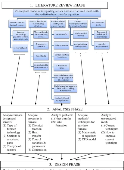
Figure 1.1a. The framework of the research – part 1.
Figure 1.1a. The framework of the research – part 1. 1. LITERATURE REVIEW PHASE
Analyze furnace design and sensors: (1)Type of
furnace technology (2)Sections & associated parts (3)The type of
sensors Analyze processes in furnace: (1)Chemical reaction (2)Heat transfer (3)Control variables & parameters (4)Combustion Analyze problem: (1)Heat transfer (2)Coke formation Analyze methods/ techniques for ethylene furnace: (1)Mathematic al equations (2)CFD model
Analyze unstructured mesh: (1)Current
techniques (2)How to
improve current technique 2. ANALYSIS PHASE
3. DESIGN PHASE
Design and develop a few version of algorithm for unstructured mesh. Design and developa conceptual model of integrating sensor and unstructured mesh with radiative heat transfer equation in order to obtain desired parameters (temperature and radiative heat flux).
Figure 1.1b. The framework of the research – part 2.
1.5 Significance of the research
This research will contribute in improving the approach of modeling and simulation study in an ethylene furnace where most of the current techniques use only existing mesh generation software (GAMBIT etc) and CFD solver software (FLUENT, SPYRO etc) to predict the performance and behavior of operating parameters in the furnace operations. Since temperature plays a significant role in the daily operation of the ethylene furnace, it is of great importance to monitor the flue gas temperature distribution in the furnace, the radiative heat flux as well as the temperature of the reactor coils. This proactive approach of coupling a set of sensors in the furnace environment will provide continuous monitoring for further action to the furnace operator and engineers.
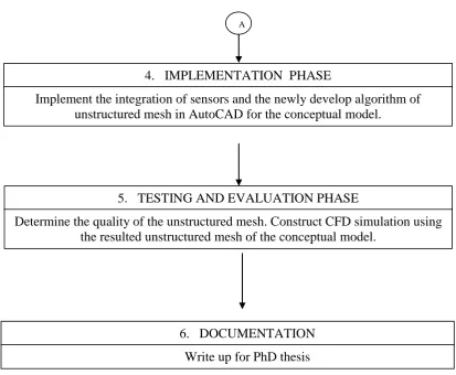
A
4. IMPLEMENTATION PHASE
Implement the integration of sensors and the newly develop algorithm of unstructured mesh in AutoCAD for the conceptual model.
5. TESTING AND EVALUATION PHASE
Determine the quality of the unstructured mesh. Construct CFD simulation using the resulted unstructured mesh of the conceptual model.
Therefore, a conceptual model of integrating sensor network and radiative heat transfer in the ethylene furnace environment is crucial as an initial phase of incorporating the ideas to the real world application. Sensors will be used to provide input in the form of boundary values for the simulation. Furthermore, the framework of the conceptual model provides the algorithm of initial triangular unstructured mesh where it incorporates the sensors deployment and a way of gradual mesh control. Besides that, it must be noted that the algorithm of the initial unstructured mesh is capable of constructing the triangular element directly in every iteration without having to re-order the front or delete the existing element as highlighted in the literature.
1.6 Outline of the thesis
An overview of the whole research is presented in Chapter 1 of the thesis. The research background of the ethylene furnace as well as the existing method of unstructured mesh formation is briefly described in the early part of the chapter. This is continued with the problem statements, the objectives and scope of the research as well as the research methodology and the significance of the research. The literature review is presented in Chapter 2 while a few versions of the unstructured mesh algorithm are developed and discussed from Chapter 3 through Chapter 5.
discretisation techniques are also described. At the end of the chapter, a review of the types of temperature sensors is presented.
Chapter 3 addressed the current problems in the element creation procedure of the standard advancing front technique. This problem has become a motivational reason of the need to enhance the current techniques in terms of element creation procedure. The first version of the newly developed algorithm for the unstructured mesh in this research is called as Enhanced Advancing Front Technique-1 (EAFT-1). The creation of the element in EAFT-1 is based on the five structured cases whereas the original technique has only two cases. The EAFT-1 is applied at a simple problem with enclosed wall where there is no inner boundary. The resulted unstructured mesh from the algorithm of EAFT-1 is integrated with the radiation model in order to proof that the mesh is appropriate for further analysis.
The second version of the unstructured mesh in Chapter 4 is called as Enhanced Advancing Front Technique-2 (EAFT-2). The element creation procedure in EAFT-2 is based on six structured cases. The radius of the circle during the element creation procedure does not follow the empirical rule as in SAFT but instead it is simpler than that. The departure zone for the element creation is set to be the entire front starting with the shortest edge. The algorithm of EAFT-2 incorporates the sensors as the boundary nodes forming boundary element. In order to tolerate the smaller size of element span over the shortest edges and the bigger size of the boundary element, the layer concept is introduced for internal gradation control of the mesh size. The EAFT-2 is applied at two simple conceptual models where in both conceptual model, the sensors are assumed to be placed along the wall. At the same time, the numbers of reactor coils in both simple conceptual models are reduced to only one complete reactor coil and half of the complete one reactor coil respectively.
edge. The departure zone for the element creation is set to be the specific front starting with the shortest edge. Similar to the approach introduced in Chapter 4, the layer concept is used for mesh size internal gradation control. A newly developed post-processing procedure to improve the quality of the mesh is also introduced in which it is called as 3 polygon refinement procedure. The algorithm of EAFT-3 is applied to the conceptual model which is designed and developed for ethylene furnace. The configuration of the ethylene furnace for the conceptual model followed the one in [33] and it is assumed that there is a set of sensors placed along the wall. The function of the sensors is to provide valuable input in the form of boundary value. At the end of the chapter, the resulted unstructured mesh incorporated with the conceptual model is applied for radiation problem in FLUENT software. The simulation converged and the desired parameters such as the flue gas temperature distribution, circumferential radiative heat flux and the circumferential skin temperature at the reactor coils are obtained.
REFERENCES
1. Hensman, A., Focus on ethylene, in Chemical week. 2009, ProQuest Central. p. S3.
2. Burridge, E., Ethylene, in European Chemical News. 2005, ProQuest Central. p. 26.
3. Gielen, D., K. Bennaceur, and C. Tam, IEA Petrochemical Scenarios for 2030-2050: Energy Technology Perspectives, in International Workshop on Technology Learning and Deployment. 2007, IEA: Paris.
4. Picciotti, M., Novel ethylene technologies developing but steam cracking remains king. Oil & Gas Journal, 1997. 95(25).
5. Han, Y., R. Xiao, and M. Zhang, Combustion and Pyrolysis Reactions in a Naphtha Cracking Furnace. Chemical Engineering & Technology, 2006. 30(1): p. 112-120.
6. Guihua, H., W. Honggang, and Q. Feng, Numerical simulation on flow, combustion and heat transfer of ethylene cracking furnaces. Chemical engineering science, 2011. 66(8): p. 1600-1611.
7. Habibi, A., B. Merci, and G.J. Heynderickx, Impact of radiation models simulations of steam cracking furnaces. Computer and Chemical Engineering 2007. 31: p. 1389-1406.
8. Nouwen, W., et al., Simulation tools evaluate large-capacity furnace designs. Oil & Gas Journal, 1998. 96(12).
9. Cremer, M., et al. Improving the performance of process heaters through fireside modeling. in AFRC International Symposium. 1997. Chicago. 10. Aminian, J., S. Shahhosseini, and M. Bayat2, Investigation of temperature
and flow Fields in an Alternative Design of Industrial Cracking Furnaces Using CFD. Iranian Journal of Chemical Engineering, 2010. 7(3): p. 61-73. 11. Heynderickx, G.J. and M. Nozawa, High-emissivity Coatings on Reactor
Tubes and Furnace Walls in Steam Cracking Furnaces. Chemical Engineering Science, 2004. 59: p. 5657-5662.
12. Modest, M.F., Radiative Heat Transfer. 2 ed. 2003: Academic Press. 822. 13. Stefanidis, G., et al., Gray/nongray gas radiation modeling in steam cracker
CFD calculations. AIChE Journal, 2007. 53(7): p. 1658–1669.
14. Koomullil, R., B. Soni, and R. Singh, A comprehensive generalized mesh system for CFD applications. Mathematics and Computers in Simulation, 2008. 78: p. 605-617.
15. Farrashkhalvat, M. and J.P. Miles, Basic structured grid generation with an introduction to unstructured grid generation. 2003: Butterworth Heinemann. 16. Lyra, P.R.M. and D.K. Carvalho, A computational methodology for
17. Rebay, S., Efficient unstructured mesh generation by means of delaunay triangulation and Bowyer-Watson algorithm. Journal of Computational Physics, 1993. 106(1): p. 125-138.
18. Teng, S.-H. and C.W. Wong, Unstructured mesh generation: Theory, practice and perspectives. International Journal of Computational Geometry and Applications, 2000. 10(3): p. 227-266.
19. Lohner, R., Progress in Grid Generation via the Advancing Front Technique. Engineering with Computers, 1996: p. 186-210.
20. Mavriplis, D.J., Unstructured grid technique. Annual Review Fluid Mechanics, 1997: p. 473-514.
21. Bathe, K.-J., Current directions in meshing, in Mechanical Engineering. 1998, ProQuest Central.
22. Muylle, J., P. Ivanyi, and B.H.V. Topping, A new point creation scheme for uniform Delaunay triangulation. Engineering Computations, 2002. 19: p. 707-735.
23. Liseikin, V.D., Unstructured Methods, in Grid Generation Methods. 2010, Springer
24. Cebeci, T., et al., Grid Generation, in Computational Fluid Dynamics for Engineers. 2005, Springer Berlin Heidelberg. p. 263-294.
25. El-Hamalawi, A., A 2D combined advancing front-Delaunay mesh generation scheme. Finite elements in analysis and design, 2004. 40: p. 967-989.
26. Muller, J.D., P.L. Roe, and H. Deconinck, A frontal approach for internal node generation in delaunay triangulations. International Journal for Numerical Methods in Fluids, 1993. 17: p. 241-255.
27. Mavriplis, D.J., An Advancing Front Delaunay Triangulation Algorithm Designed for Robustness. Journal of Computational Physics, 1995. 117(1): p. 90-101.
28. Mavriplis, D.J., Unstructured mesh generation and adaptivity. 1995, Institute for Computer Applications in Science and Engineering (ICASE.
29. Frey, P.J., H. Borouchaki, and P.-L. George, 3D Delaunay mesh generation coupled with an advancing-front approach. Computer methods in applied mechanics and engineering, 1998. 157: p. 115-131.
30. Radovitzky, R. and M. Ortiz, Tetrahedral mesh generation based on node insertion in crystal lattice arrangements and advancing-front-Delaunay triangulation. Computational Methods in Applied Mechanics and Engineering., 2000. 187: p. 543-569.
31. Sahimi, M., et al., Upscaled unstructured computational grids for efficient simulation of flow in fractured porous media. Transport in Porous Media, 2010. 83(1): p. 195-218.
32. Kovac, N., S. Gotovac, and D. Poljak, A New Front Updating Solution Applied to Some Engineering Problems. Archives of Computational Methods in Engineering, 2002. 9: p. 43-75.
33. Lan, X., et al., Numerical Simulation of Transfer and Reaction Processes in Ethylene Furnaces. Chemical Engineering Research and Design, 2007. 85(A12): p. 1565-1579.
34. Zimmermann, H. and R. Walzl, Ethylene. 2005, Linde AG.
36. Heyndericks, G.J., G.G. Cornelis, and G.F. Froment, Circumferential tube skin temperature profiles in thermal cracking coils. AIChE Journal, 1992. 38(12): p. 1905-1912.
37. Bockelie, M.J., et al. Computational simulations of industrial furnaces. in International Symposium on Computational Technologies For
Fluid/Thermal/Chemical System with Industrial Applications. 1998. California, USA.
38. Hillewaert, L.P., J.L. Dierickx, and G.F. Froment, Computer generation of reaction schemes and rate equation for thermal cracking. AIChE Journal, 1988. 34(1): p. 17-24.
39. Edwin, E.H. and J.G. Balchen, Dynamic optimization and production planning of thermal cracking operation. Chemical Engineering Science, 2001. 56: p. 989-997.
40. Karimzadeh, R., H.R. Godini, and M. Ghashghaee, Flowsheeting of steam cracking furnaces. Chemical Engineering Research and Design, 2009. 87: p. 36-46.
41. Masoumi, M.E., et al., Simulation, optimization and control of a thermal cracking furnace. Energy, 2006. 31: p. 516-527.
42. Niaei, A., et al., The combined simulation of heat transfer and pyrolysis reactions in industrial cracking furnaces. Applied Thermal Engineering, 2004. 24: p. 2251-2265.
43. Goethem, M.W.M.V., et al., Towards synthesis of an optimal thermal cracking reactor. Chemical Engineering Research and Design, 2008. 86: p. 703-712.
44. Geem, K.M.V., M.F. Reyniers, and G.B. Marin, Challenges of Modeling Steam Cracking of Heavy Feedstocks. Oil & Gas Science and Technology 2008. 63(1): p. 79-94.
45. Yu, S., Modelling and Simulation of Hydrocarbon Cracking, in School of Engineering. 2007, Cranfield University. p. 88.
46. Sadrameli, S.M. and A.E.S. Green, Systematics and modeling representations of naphtha thermal cracking for olefin production. Journal of Analytical and Applied Pyrolysis, 2005. 73: p. 305-313.
47. Stefanidis, G.D., et al., Evaluation of high-emissivity coatings in steam cracking furnaces using a non-grey gas radiation model. Chemical Engineering Journal, 2008. 137: p. 411-421.
48. E, J., et al., CRACKER - A PC Based Simulator for Industrial Cracking Furnaces Computers and Chemical Engineering, 2000. 24: p. 1523-1528. 49. Furnaces, Heaters and Incinerators. [cited 2011; Available from:
linde-engineering.com.
50. Stefanidis, G., et al., CFD simulations of steam cracking furnaces using detailed combustion mechanisms. Computers & Chemical Engineering, 2006. 30(4): p. 635-649.
51. Heynderickx, G.J., et al., Three-Dimensional Flow Patterns in Cracking Furnaces with Long-Flame Burners. AIChE Journal, 2001. Vol. 47, No. 2: p. 388-400.
52. Brown, D.J., et al. Fireside modeling in cracking furnaces. in AIChE 9th Annual Ethylene Producers Conference. 1997. Houston, USA.
53. Tang, Q., et al. Advanced CFD Tools for Modeling Lean Premixed
54. Rahman, N.S.A., et al., The state of the art for ethylene cracking furnace modeling. 2008, Universiti Teknologi Malaysia.
55. Li, C., et al., Fluid dynamic numerical simulation coupled with heat transfer and reaction in the tubular reactor of industrial cracking furnaces.
International Journal for Numerical Methods in Fluids, 2009. 62(4): p. 355-373.
56. Belohlav, Z., P. Zamostny, and T. Herink, The kinetic model of thermal cracking for olefins production. Chemical Engineering and Processing, 2003: p. 461-473.
57. Cai, H., A. Krzywicki, and M.C. Oballa, Coke formation in steam crackers for ethylene production. Chemical Engineering and Processing, 2002: p. 199– 214.
58. Schools, E.M. and G.F. Froment, Simulation of decoking of thermal cracking coils by steam/air-mixtures. AIChE Journal, 1997. 43(1): p. 118-126.
59. Guo, Z., Z. Fu, and S. Wang, Sulfur distribution in coke and sulfur removal during pyrolysis. Fuel Processing Technology, 2007. 88: p. 935-941.
60. Hájeková, E., et al., Coke Formation during copyrolysis of polyalkenes with naphtha. Petroleum & Coal, 2008: p. 52-55.
61. Colannino, J., Ethylene furnace heat flux correlations. 2008.
62. Oprins, A.J.M. and G.J. Heynderickx, Calculation of three-dimensional flow and pressure fields in cracking furnaces. Chemical Engineering Science, 2003: p. 4883 – 4893.
63. Li, B.Q., Discontinuous Finite Elements in Fluid Dynamics and Heat Transfer. 2006, Germany: Springer-Verlag. 586.
64. Versteeg, H.K. and W. Malalasekera, An Introduction to Computational Fluid Dynamics. 2007, England: Pearson Education.
65. Owen, S.J. A survey of Unstructured Mesh Generation Technology. in International Meshing Roundtable 1998. Dearborn, Michigan
66. Blazek, J., Principles of Grid Generation, in Computational Fluid Dynamics: Principle and Applications. 2007.
67. Peraire, J., J. Peiro, and K. Morgan, Advancing front grid generation, in Handbook of Grid Generation, N.P. Weatherill, B.K. Soni, and J.F. Thompson, Editors. 1999, CRC Press LLC.
68. George, A.J., Computer Implementation of the Finite Element Method, in Department of Computer Science. 1971, Stanford University.
69. S.H.Lo, A New Mesh Generation Scheme for Arbitrary Planar Domains. International Journal for Numerical Methods in Engineering, 1985. 21: p. 1403-1426.
70. Persson, P.-O., Lecture 1 Computational Mesh Generation. 2008, MIT. 71. Zhu, J., T. Blacker, and R. Smith, Background overlay grid size functions, in
Proceedings of the 11th international meshing roundtable. 2002. p. 65–74. 72. Seveno, E. Towards an adaptive advancing front method. in 6th International
Meshing Roundtable. 1997.
73. Naji, H.S., An improved advancing front algorithm for triangulating arbitrary two dimensional regions. 2004.
74. Minyi, K., C. Jie, and J. Huazhong, Research of Using Dynamic Programming in the Nodes Encoding Optimization, in International
Conference on Information Engineering and Computer Science, 2009. 2009. 75. Ito, Y., et al., Parallel unstructured mesh generation by an advancing front
76. Sazonov, I., et al., A stitching method for the generation of unstructured meshes for use with co-volume solution techniques. Computational Methods in Applied Mechanics and Engineering., 2006. 195: p. 1826–1845.
77. Hernández-Mederos, V., P.L.d. Ángel, and J. Estrada-Sarlabous, Isotropic umbrella based triangulation of regular parametric surfaces. Numer Algor, 2008. 48: p. 29–47.
78. Wang, W.X., C.Y. Ming, and S.H. Lo, Generation of triangular mesh with specified size by circle packing. Advances in Engineering Software, 2007. 38: p. 133-142.
79. Owen, S.J. An Introduction to Mesh Generation Algorithm. in 14th International Meshing Roundtable. 2005. San Diego, California, USA. 80. Okusanya, T.O., An algorithm for parallel unstructured mesh generation and
flow analysis, in Department of Aeronautics and Astronautics. 1996, Massachusetts Institute of Technology. p. 119.
81. Tremel, U., et al., Parallel generation of unstructured surface grids. Engineering with Computers, 2005: p. 36-46.
82. Sorli, K., A Review of Computational Strategies for Complex Geometry and Physics. 2002, CFD Applied to Reactor ProcEss Technology.
83. George, P.L. and E. Seveno, The advancing front mesh generation method revisited. International Journal for Numerical Methods in Engineering, 1994. 37: p. 3605-3619.
84. Vasiliauskiene, L. and R. Bausys, Intelligent Initial Finite Element Mesh Generation for Solutions of 2D Problems. INFORMATICA, 2002. 13: p. 239–250.
85. Vasiliauskiene, L., Adaptive finite element strategies for solution of two dimensional elasticity problems, in Technological Sciences, Mechanical Engineering. 2006, VILNIUS GEDIMINAS TECHNICAL UNIVERSITY. 86. Chong, C.S., A. Senthil Kumar, and H.P. Lee, Automatic mesh-healing
technique for model repair and finite element model generation. Finite elements in analysis and design, 2007. 43(15): p. 1109-1119.
87. Schoberl, J., NETGEN An advancing front 2D/3D - mesh generator based on abstract rules. Computing and Visualization in Science, 1997: p. 41-52. 88. Liu, J., H.M. Shang, and Y.S. Chen, Development of an unstructured
radiation model applicable for two-dimensional planar, axisymmetric, and three-dimensional geometries. Journal of Quantitative Spectroscopy & Radiative Transfer 2000. 66: p. 17-33.
89. Li, B.Q., Radiative Transfer in Participating Media, in Discontinuous Finite Elements in Fluid Dynamics and Heat Transfer, K.-J. Bathe, Editor. 2006, 3: Germany.
90. Lacanette, K., National Temperature Sensor Handbook. 1997: National Semiconductor. 42.
91. Chen, J., X. Hu, and L. Xu, A New T hermocouple Auto-Calibration System, in International Conference on Computer Science and Software Engineering. 2008, IEEE.
92. Zhang, M., Research and Implement of Thermocouple Sensor and Microcontroller Interface. 2010, IEEE.
93. Sensor Types and Principles of Operation, Testemp Ltd. 94. RTD Theory, SensorTec Inc.
96. Wobschall, D. and W.S. Poh, A Smart RTD Temperature Sensor with a Prototype IEEE 1451.2 Internet Interface in Senson for Industry Conference. 2004, IEEE: New Orleans, Louisiana, USA.
97. Dogan, I., Chapter 5 - Thermistor Temperature Sensors, in Microcontroller Based Temperature Monitoring and Control. 2002, Newnes: Oxford. p. 107-127.
98. (2003) Introduction to AutoCAD LT. Volume,
99. Gambit 2.3 Documentation - Gambit User Guide. [cited 2010 25 November]; Available from:
http://my.fit.edu/itresources/manuals/gambit2.3/help/index.htm.