High Dimensional Methods in Statistics, Data Mining and Finance.

(1)

ABSTRACT

SAHOO, SASWATA. High Dimensional Methods in Statistics, Data Mining and Finance. (Under the direction of Soumendra Nath Lahiri.)

This dissertation focuses on some applications of high dimensional methods in statistics,

data mining and finance. A nonparametric method for evaluating confidence region of high

dimensional functional parameters is developed. Evaluation of confidence region of high

di-mensional functional has some difficulties which are investigated and remedial solutions are

provided. Some aspects of multidimensional data visualization and data mining are explored.

A scalable clustering algorithm is developed. An application of resampling method in high

dimensional financial portfolio construction is studied.

We give a brief outline of the thesis in Chapter 1. In Chapter 2, we focus on evaluating

con-fidence region of high dimensional functional parameter of the parent population. Extension of

traditional empirical likelihood method is shown to fail in high dimension and we propose a

suitable penalized empirical likelihood ratio which is shown to efficiently handle high

dimen-sional functionals. Numerical Performance of the proposed method is also investigated.

Confidence region of a finite dimensional functional parameter is generally evaluated by

grid search method. However, for parameters which are high dimensional or even of moderately

large dimension, grid search method is either completely infeasible or computationally quite

intensive. In Chapter 3, two methods are developed to construct confidence region of such

functional parameters, one of them is based on smoothing followed by a grid searching and the

other is based on bootstrap resampling. Visualization of the confidence region is a challenge in

high dimensional functional space. A visualization of the confidence region based on minimum

volume ellipsoid covering suitable list of candidates of the confidence region is possible. The

(2)

Data visualization has lot of limitations for high dimensional data or even for

multivari-ate data with modermultivari-ate dimension. Minimum volume ellipsoid covering of multivarimultivari-ate data is

utilized to develop a boxplot for high dimensional data. A subsampling based scalable

cluster-ing algorithm which is particularly useful for big datasets is proposed. The algorithm can be

conveniently implemented in Hadoop clusters. We describe these methods in Chapter 4.

In financial portfolio construction, high dimensional covariance matrices are encountered

and under growing dimension, maximum likelihood estimation of covariance matrix does not

work. In Chapter 5, we consider the celebrated Markowitz mean variance portfolio

optimiza-tion problem in high dimension. A regularized estimator of high dimensional covariance of

stocks cross correlation is implemented. There is no result in the literature regarding

confi-dence interval of optimized portfolio risk. Under growing number of stocks in the portfolio,

sparse characterization of the stock cross-covariance matrix and temporal dependence of stock

returns, we implement resampling method to evaluate confidence interval of optimized

portfo-lio risk. “Out of sample" performance of the portfoportfo-lio strategy is investigated using real data

(3)

(4)

High Dimensional Methods in Statistics, Data Mining and Finance

by Saswata Sahoo

A dissertation submitted to the Graduate Faculty of North Carolina State University

in partial fulfillment of the requirements for the Degree of

Doctor of Philosophy

Statistics

Raleigh, North Carolina

2014

APPROVED BY:

Howard Bondell Lexin Li

Daowen Zhang Soumendra Nath Lahiri

(5)

DEDICATION

(6)

BIOGRAPHY

Saswata Sahoo was born to Dr. Dilip Kumar Sahoo and Banani Sahoo in the year 1989 in

Kolkata, India. He went to Jadavpur Vidyapith and then Ramakrishna Mission Residential

College, Narendrapur for his secondary and higher secondary study respectively. He received

B.Sc degree in Statistics from Ramakrishna Mission Residential College, Narendrapur and then

went to University of Calcutta for the master degree. He got interested in Financial Statistics

and after completing M.Sc in Statistics in the year 2011 from University of Calcutta, he joined

department of Statistics, Texas A & M University at College Station in Texas to work towards

his Ph.D under the guidance of Dr. Soumendra Nath Lahiri. Later in the year 2012, Dr. Lahiri

moved to North Carolina State University at Raleigh in North Carolina and he generously

took Saswata with him to the wonderful Statistics department. There, Saswata developed some

keen interest in problems related to Big Data and his focus of research shifted to the new

domain. Apart from Statistics, Saswata has some crazy interest in cars. One day he surely

wants to own some his favorite cars. He likes to travel and landscape photography came to him

almost immediately as he started traveling some of the most wonderful places on earth. Cricket,

Rabindranath Tagore’s songs and delicious Indian food, these are the three important things

Saswata cannot live without. After completion of his PhD, he is going to join the Advance

(7)

ACKNOWLEDGEMENTS

First of all, I would like to thank my advisor, Dr. Soumendra Nath Lahiri, whose constant

aca-demic and moral support has made it possible for me to stay in USA for three years, almost

18 thousand kilometers away from home. In spite of him being such a celebrated and

accom-plished scientist with a busy day to day schedule, I shall never forget the kind of care and

warmth I have received from him through out these three years of my stay under his guidance.

I have no word to acknowledge the support I got from my friends here in USA. I would

never forget the kind of welcome I received from Shahina Rahman and Sourav Dutta when I

first arrived USA. I would love to specially thank Arka dasgupta, Ya Su, Sen Mao, Subhadeep

Mukhopadhyay, Debkumar De with whom I spent a wonderful year in Texas. Later, in North

Carolina, life became wonderful due to the constant support and presence of my lovely group of

talented friends Mangesh Champhekar, Rajarshi Das Bhowmik, Prithwish Bhaumik, Sayantan

Banerjee, Shuva Gupta, Debraj Das and Priyam das.

My parents, like all parents in the world, have always been a safe shelter whenever I faced

tough times and we all weathered out the storm together. There is no word to describe the

kind of support I got from my uncle, Sandip Sahu who has always been instrumental in taking

many important decisions in my life. I would like to specially thank Rudrodip Majumdar and

Debarati Bhattacharya who extended their hands whenever I needed them and I am sure they

will continue to do so for ever.

My heartiest thanks to all my teachers. I would specially like to thank Department of

Statis-tics at Ramakrishna Mission Residential College, Narendrapur which perhaps has been the

most important part of my life as far as my academic and professional career are concerned.

Finally I thank all my committee members, Dr. Lexin Li, Dr. Howard Bondell and Dr. Daowen

(8)

LIST OF TABLES

Table 2.1 The difference|α−α|ˆ of the empirical size ( ˆα) and nominal size (α) of the empirical likelihood ratio test forH0 based onN =500 replications

for varying values ofnandp. . . 28 Table 2.2 Coverage accuracy of the confidence regions for the subsampling based

cut-off points of limit distribution of PEL under various subsampling size where desired coverage accuracy is 0.90 . . . 29 Table 2.3 Coverage accuracy and average length of the estimated confidence

re-gion for the quantile function when the nominal coverage level is 0.90 . . 30 Table 2.4 Coverage accuracy and average length of the estimated confidence

re-gion for the quantile function corresponding to incomplete data when the nominal coverage level is 0.90 . . . 31

Table 3.1 Results related to empirical coverage probability (Cov. Prob), average length (Avg. Len), minimum (Min. Len) and maximum length (Max. Len) for quantile functionξ[0.70,0.95,F] ={ξη(F),η ∈[0.70,0.95]} whereF=exp(1) . . . 57 Table 3.2 Results related to empirical coverage probability (Cov. Prob), average

length (Avg. Len), minimum (Min. Len) and maximum length (Max. Len) for quantile functionξ[0.70,0.95,F] ={ξη(F),η ∈[0.70,0.95]} whereF=χ₃2 . . . 58 Table 3.3 Computation time in seconds, in an Intel Core i5, 2.4 GHz processor

with 8 GB memory, for estimations of the confidence region for quan-tile function{ξ_η(F),η∈[0.70,0.95]}for the different choices ofn,c∗, nominal level and parent populations. . . 58

Table 4.1 Results related to discovery of the clusters of different simulated data under varying data dimension and true number of clusters. . . 95 Table 4.2 Results related to proportion of misclassification for varying data

dimen-sion, window size and size of the dataset. . . 96 Table 4.3 Description of Clusters obtained from Iris Data. . . 98

Table 5.1 Sharpe’s Ratio (SR) and the difference between out of sample portfo-lio mean ˆµout compared the desired expected return µ0 corresponding

(11)

Table 5.2 Coverage accuracy and average length of the estimated confidence in-terval of the optimized risk where the desired coverage level is 0.90 and ρ1=0 . . . 118

Table 5.3 Coverage accuracy and average length of the estimated confidence in-terval of the optimized risk where the desired coverage level is 0.90 and ρ1=0.1 . . . 119

Table 5.4 Coverage accuracy and average length of the estimated confidence in-terval of the optimized risk where the desired coverage level is 0.90 and ρ1=0.3 . . . 120

(12)

LIST OF FIGURES

Figure 2.1 The projection of the confidence region of (ξη1, . . . ,ξη4,ξη∗,ξη5)on the

3 dimensional space of(ξη₄,ξη∗,ξη5)obtained by taking convex

com-binations of the confidence limits of the neighboring points ofξη∗. The

projection turns out to be a flat plane instead of a 3 dimensional solid object. Different projections are obtained by choosing different weights of the convex combinations. The true value is represented by the red dot which actually is outside all the planes. . . 10 Figure 2.2 The projection of the confidence region of (ξη₁, . . .ξη₄,ξη∗,ξη5)

ob-tained by interpolation on the 3 dimensional space of (ξη4,ξη∗,ξη5).

The projection turns out to be a flat plane instead of a 3 dimensional solid object. The true value is represented by the red dot which actually is outside the plane. . . 11 Figure 2.3 3 dimensional projection of the p_n dimensional confidence region on

the space of (ξη₄,ξη∗,ξη5). PELR based confidence set contains the

truth shown as red colored dot. . . 17 Figure 2.4 For n=1200, under varying p, the qqplot of the observed empirical

likelihood ratio against normal distribution . . . 27

Figure 3.1 3 dimensional feasible region of quantiles over only three points on the grid, η1,η2,η3, i.e. (ξη1,ξη2,ξη3), satisfying ξη1 ≤ξη2 ≤ξη3 and the

desired confidence region enclosed inside it. . . 38 Figure 3.2 Bootstrap replicates will result in a list of candidates{ξ∗[a,b,Fˆ∗(l)],l=

1,2, . . . ,B_boot}of the confidence region which will cover the target re-gionB(χn)well. The members from this bootstrap list which satisfy the likelihood ratio criteria are cropped out. . . 47 Figure 3.3 For the smoothing method, the shift is performed on a reasonably fine

grid of functional in the functional space, so that, as we move along the grids, the likelihood exhibits a very prominent monotonic nature at either side of the maximum. The search procedure starts atd=0 and is continued in both the directions, i.e. ford=±1,±2,±3. . .etc. . . 49 Figure 3.4 Taking 3 quantiles at a time from the p_ndimensional discretized

quan-tile function, representation of the confidence region by taking projec-tions of the pn dimensional ellipsoid on the respective 3 dimensional Euclidean spaces. . . 54 Figure 3.5 Region enclosed by the p_n dimensional candidates of the confidence

(13)

Figure 4.1 Boxplot for model 1 withn=100 forη =1 and η =7. The red dots represent the outliers and the black dots represent the inliers. The in-ner ellipsoid, which is shown in green color is the MVE of inin-ner 50% observations and the outer ellipsoid is shown in blue color . . . 70 Figure 4.2 3 dimensional projection of the boxplots for p=4 and n=100 and

Model 2. The inner ellipsoids are denoted by green color and the outer ellipsoids are denoted by blue color. The inliers are shown as black points inside the ellipsoids and the outliers are denoted by red points. . 71 Figure 4.3 3 dimensional projection of the boxplots for p=4 and n=100 and

Model 3. The inner ellipsoids are denoted by green color and the outer ellipsoids are denoted by blue color. The inliers are shown as black points inside the ellipsoids and the outliers are denoted by red points. . 72 Figure 4.4 Outlier detection results for model 2 and model 3 with n=100 and

p=50. The inliers are denoted by the black curves and the outliers are denoted by the red curves. . . 73 Figure 4.5 Ellipsoid covering of chunks which are close to each other and which

are distant from each other . . . 78 Figure 4.6 MapReduce architecture . . . 85 Figure 4.7 The left panel shows two chunks which are significantly overlapped

with dissimilarity value in the range(1/2,1)where as the right panel exhibits two weakly overlapped chunks with dissimilarity values greater than 1 . . . 89 Figure 4.8 MapReduce implementation of the clustering algorithm . . . 91 Figure 4.9 Dendogram of the cluster analysis of Iris data. . . 97 Figure 4.10 Scatter plot of the Iris data with 4 variables (X,Y,Z,W), taking only

(14)

Chapter 1 Introduction

With the recent advancement of science and technology, slowly but surely, Statistics has been

going through lot of interesting changes. There have been changes in the core philosophy, in

the methodologies and most importantly, in its range of applicability. As Donoho (2000) rightly

pointed out, a combination of blind faith and serious purpose has led the society to invest

mas-sively on data at an unimaginable scale. That has triggered statisticians to think about high

di-mensionality of the data where the challenge is to simultaneously handle information on a large

number of features on the experimental units. The other side of the coin has received attention

relatively recently, to be specific in the last 5 years. Data have grown in size unimaginably in

the last few years from different scientific, economic and business communities. Essentially

one needs to process and analyze data of enormous volume, generated at lightning velocity

and of all structures. The term “Big Data" has become the buzz word and computer scientists,

engineers, statisticians, mathematicians have joined hands in the process of redefining the art

of learning from such datasets. DNA Microarrays, internet portals, financial investments,

elec-tronic censors, social community, GPS tracking, airline ticketing, medical image processing,

(15)

interest is to study scope of some high dimensional statistical methods in estimation, analysis

and decision making process.

High dimensional population parameters such as quantile function, regression function,

regression coefficients etc. are important in statistics and econometrics. Nonparametric

sta-tistical estimation techniques of such quantities supply important information on the parent

population. Point estimates fail to provide enough information on the statistical uncertainty

that is associated with the inferential process. A confidence region of appropriate confidence

level often gives a more informative and comprehensive picture of the parameter of interest. In

Chapter 2 we develop a nonparametric method based on empirical likelihood which is capable

of supplying confidence region of very high dimensional functional parameter. We particularly

focus in the quantile function.

The confidence region of high dimensional functional is hard to construct and visualize

even at the cost of significant computation power. The confidence region evaluation technique

developed in Chapter 2, theoretically is very accurate in quantifying the sampling variation at

functional level, but it does not have the convenience of an easy representation like a

tradi-tional confidence region. In fact, the exact region is almost unattainable. Such problems are

not uncommon in machine learning and data mining literature. But, in the context of statistical

confidence region estimation, there is hardly any previous work to resolve such difficulties. We

deal the problem somewhat pragmatically and come up with some approximate solutions in

Chapter 3. We propose two methods to come up with approximate confidence region of high

dimensional functional parameters. Based on a list of members of the high dimensional

con-fidence region in the functional space, we also attempt to adopt minimum volume ellipsoid

covering to approximate the desired confidence region.

The minimum volume ellipsoid covering a collection of points in the high dimensional

(16)

some explorable potential in statistical learning problems too. We investigate on its potential

as multi dimensional data visualization and develop a multidimensional boxplot in Chapter

4. We develop a scalable clustering algorithm based on a without replacement subsampling

scheme with minimum volume ellipsoid. A clustering problem, in its simplest form, can be

described as a problem of allocating data points to a number of subclasses so that the within

subclasses variation is minimized and between subclasses variation is maximized. We look at

clustering from a different perspective which is new and seems quite promising in the context

of big data. It is not hard to appreciate the fact that, there might be huge number of observed

data points but the relevant region in the multidimensional feature space is bounded in most

practical situations. The feature space can be gridded by blocks of suitable geometric shape

of corresponding dimension. Algorithm in terms of finitely many blocks that grid the feature

space, instead of the huge number of observed points themselves, seem more tractable in the

context of clustering of big data. We focus on ellipsoidal blocks to grid the feature space. We

develop a subsampling scheme aided with minimum volume ellipsoid in such a way that it

extracts ellipsoidal blocks in the feature space with high density chunks of points. Eventually

the clusters are discovered by pruning the similar chunks from the feature space. The algorithm

has the quality to be implemented in a distributed file system, which looks quite promising in

the context of big data.

Due to the recent advancement of risky trading strategies, globalization of banks and

dereg-ulation of market all over the world, risk associated with financial affairs has increased several

folds. In fact, trading methodology has advanced to such level, that the risk is no more a

fear,-rather it is looked upon as a trading instrument by serious investors. Risk is actually the

pre-mium, one possibly needs to pay to earn the extra profit. It is possible to hold a financial

position in such a way that a significant amount of risk can be diversified among different

(17)

to the multi directional industrial growth and increasing ease of trading beyond geographical

boundary, the pool of financial stocks or instruments available to diversify the risk is practically

unbounded in numbers. The optimum portfolio construction diversifying the risk on unbounded

number of stocks or instruments is essentially a high dimensional problem. The sampling

vari-ation associated with the portfolio risk estimvari-ation is subjected to the difficulties associated with

high dimensional statistical methods. Beyond certain number of stocks or financial instruments

involved in the portfolio formation, it becomes difficult to estimate the risk of the holding

port-folio. In Chapter 5, we implement a resampling method to numerically investigate the effect of

dimensionality on estimation of portfolio risk when there is temporal dependence among stock

(18)

Chapter 2 Empirical Likelihood Method for High

Dimensional Functional Parameters

2.1 Introduction

Empirical likelihood, introduced by Owen (1990, 1988) has gained popularity in

nonparamet-ric and semi parametnonparamet-ric method due to its two elegant and convenient features- the Wilk’s

theorem and the Bertlett’s correction (cf. Hall and La Scala (1990), Diciccio (1991)). In spite

of it being a nonparametric likelihood, it has the qualities of a parametric likelihood. Owen

(1990) developed the empirical likelihood for mean functional of independent and identically

distributed finite dimensional random vector, and later, Qin and Lawless (1994) generalized

it for finite dimensional functional which are solutions of finitely many estimating equations.

For the past few years, due to the increasing availability of financial, genetic and market data,

there is a noticeable interest in high dimensional method in the scientific community. There

are some recent works on developing empirical likelihood in high dimensional framework.

(19)

dimen-sional data. On the other hand, Hjort et al. (2009) generalized empirical likelihood ratio for

functional which are solution of unboundedly many estimating equations. In this chapter, we

are particularly interested in empirical likelihood method for such high dimensional functional

parameters.

LetX₁,X2, . . ., be a sequence of independently and identically distributed random variables

on a probability space denoted by(Ω,A,P), whereΩis the sample space,A is a sigma field

of subsets ofΩ andP is a probability distribution defined on the elements ofA. Associated

with the random variable X_i on(Ω,A,P), we have a probability distribution functionF. We

observe a random sample of size n which can be denoted by χn ={X1,X2, . . . ,Xn}. In the present discussion we consider the class of functional parameters θ(F) ∈Θ which can be

expressed in terms of solutions of unboundedly many estimating equations of the form

Z

R

g_k(X₁,θ(F))dF =0 k=1,2, . . . ,p_n (2.1)

where pngrows unboundedly. The empirical likelihood ratio is constructed utilizing the infor-mation onθ(F), available from the sample average version of the estimating equations, such as

Z

R

g_k(X₁,θ(F))dFˆ =0, k=1,2, . . . ,pn

where ˆFis an appropriate estimate ofFbased onχn. Under the assumption that the distribution functionF(.)is such that it assigns some unknown but nonzero probabilities πi’s on each of the sampled observations X_i’s, such that ∑n_i₌₁πi =1 and πi >0 for all i, the unconstrained maximized data likelihood is given by

L(F_n) = max πi,i=1,2...,n

{ n

∏

i=1

πi: n

∑

i=1

(20)

For parameterθ(F)which is expressed as (2.1) the constrained maximum likelihood profiled with respect toθ(F)is defined as

˜

L(θ(F)) = max

πi;i=1,...,n

{

_∏

i

πi: n

∑

i=1

πig(Xi,θ(F)) =0, n

∑

i=1

πi=1,πi>0}.

The empirical likelihood ratio hence, is defined as the ratio

˜

R_n(θ(F)) =L˜(θ(F))/L(Fn) =nnL˜(θ(F)).

Owen (1990) showed that, one important requirement for the empirical likelihood ratio to

work is that the convex hull of

{ g₁(X_i,θ(F)),g2(Xi,θ(F)), . . . ,gp(Xi,θ(F))

∈_Rp:i=1,2, . . . ,n}

should contain the zero of_Rp . But when p= p_n→∞, Tsao (2004) found that the concerned

convex hull shrinks in size and beyond certain growth rate of pn the convex hull may not contain the 0 of_Rpn_{. To be specific, the author showed that as long as} _p

n= [(ε)n], for some ε ∈(0,1/2), the convex hull contains the 0 of _Rpn_{, where} _[_x_]_{is the largest integer contained}

in x. Moreover, even if this growth rate is satisfied, there is no assurance that the likelihood ratio ˜R_n(θ(F)) will have a non degenerate limit distribution. Since the functional parameter

(21)

the authors could prove, (2p_n)−1/2(−2 ˜R_n(θ(F))−pn)→N(0,1) as pn,n→∞. In order to overcome these slower rates, the convex hull requirement needs to be dropped from the

for-mulation. With this aim in mind Bartolucci (2007), Lahiri and Mukhopadhyay (2012b), Lahiri

and Mukhopadhyay (2012a) developed penalized empirical likelihood for mean functional to

attain increasingly faster growth rate of data dimension. In the present chapter, our goal is to

develop penalized empirical likelihood ratio for high dimensional functional parameterθ(F) as defined in (2.1).

2.2 High Dimensional Functional Parameters

2.2.1 Motivation

We are interested in empirical likelihood ratio for functional parameters which can be expressed

by the solutions of estimating equations of the form (2.1). In particular, consider quantile

func-tion defined as

ξ[a,b,F] ={ξη(F),η∈[a,b]⊂[0,1]} where ξη(F) =inf

x {x:F(x)≥η}.

The sample distribution function is given by Fn(x) =n−1∑n_i=11(Xi≤x), x∈R, which is a random variable putting mass n−1 at each of X_i’s and where we denote 1(A)as the indicator function taking value 1 or 0 according as an eventAhas occurred or not. The sample quantile function is given byξn[a,b,Fn] ={ξnη(Fn),η∈[a,b]⊂[0,1]}whereξnη(Fn) =infx{x:Fn(x)≥ η}. The quantile functionξ[a,b,F]can be discretized at pnpoints and the discretized quantile

function can be represented by the solution of thep_nestimating equations of the form

Z

R

1(X₁≤ξηk(F))−ηk

(22)

with p_n conceptually growing unboundedly with sample size n→∞. Hjort et al. (2009)

al-lowed pn to grow up to the rate pn=o(n1/3). Discretizing ξ[a,b,F] at pn=o(n1/3) points and accordingly using that many estimating equations following (2.2), the empirical likelihood

ratio of Hjort et al. (2009) provides simultaneous confidence region of (ξη1,ξη2, . . . ,ξη_pn)0. However, the rate p_n =o(n1/3) only allows very coarse gridding, and hence we have no in-formation on the confidence region at intermediate points of the discretized quantile function.

For example, withn=50 and choosing p_n=5, we have information at only 5 points of the quantile function(ξη1,ξη2, . . . ,ξη5)

0_{. To obtain a confidence region of the quantile function, it}

is important to incorporate information at finer grids which of course is not possible with the

allowable growth rate of pn=o(n1/3) at fixed sample size. Clearly the confidence region of

(ξη₁,ξη₂, . . . ,ξη₅)0 can be thought of as a collection of points in the 5 dimensional Euclidean space. It may be tempting to obtain confidence region of the quantile function at finer grids

or at intermediate region by some interpolation method. For example- suppose, based on the

confidence region of(ξη1,ξη2,ξη3,ξη4,ξη5), we might want to obtain simultaneous confidence

region for say,

(ξη1,ξη2,ξη3,ξη4,ξη∗,ξη5)

0

whereη∗∈(η4,η5). Now, the empirical likelihood ratio certainly takes into account the

sam-pling variation at the 5 chosen grid points(ξη1,ξη2,ξη3,ξη4,ξη5). But, combining confidence

limits at the neighboring grid points ofη∗, i.e. atη4andη5to obtain confidence limits ofξη∗

does not make any statistical sense. The region so obtained is not going to work as a confidence

region of

(ξη1,ξη2,ξη3,ξη4,ξη∗,ξη5)

0

in the 6 dimensional Euclidean space.This is because the sampling variations at ξη∗ will not

(23)

1 2

3 4

1 1.5

2 2.5

3 3.5

4 2 2.2 2.4 2.6 2.8 3 3.2 3.4 3.6 3.8

ξ η

1 ξ

η *

ξ η

2

Figure 2.1The projection of the confidence region of (ξη1, . . . ,ξη4,ξη∗,ξη5)on the 3 dimensional

space of(ξη4,ξη∗,ξη5)obtained by taking convex combinations of the confidence limits of the

neigh-boring points ofξη∗. The projection turns out to be a flat plane instead of a 3 dimensional solid object.

(24)

1 1.5

2 2.5

3 3.5

4

1.5 2 2.5 3 3.5 4 4.5 1.5 2 2.5 3 3.5 4 4.5 5

ξ_η 4 ξ_η_*

ξ η 5

Figure 2.2The projection of the confidence region of (ξη1, . . .ξη4,ξη∗,ξη5)obtained by interpolation

on the 3 dimensional space of(ξη4,ξη∗,ξη5). The projection turns out to be a flat plane instead of a

(25)

that one tempting way of combining confidence limits at ξη4 and ξη5 will be to take convex

combination of confidence limits of ξη4 and ξη5 to obtain the confidence limits ofξη∗. Each

member of the confidence region of(ξη1,ξη2,ξη3,ξη4,ξη∗,ξη5)is a point in the 6 dimensional

Euclidean space. Let us particularly focus to the part of the confidence region relevant to only

(ξη4,ξη∗,ξη5) for ease of understanding. Considering all the 6 dimensional members of the

region, we can imagine two vectors, one obtained by choosing and stacking the components

corresponding toξη4 and the other by stacking the components corresponding toξη5. With a

fixed weight of the convex combination, the projection of the 6 dimensional confidence region

on the 3 dimensional space of(ξη4,ξη∗,ξη5)reduces to a 2 dimensional plane instead of a solid

3 dimensional object. This is because the vector obtained by stacking the component

corre-sponding toξη∗ is linearly dependent on the two vectors corresponding toξη4 andξη5. Varying

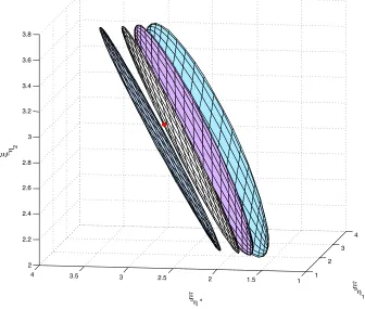
weights of the convex combinations, the simultaneous confidence region of (ξη4,ξη∗,ξη5) is

shown in figure 2.1. The true value of(ξη4,ξη∗,ξη5)is plotted as a red dot in the figure. Each

of the projections for fixed weights reduces to a 2 dimensional plane in the 3 dimensional

space. Fixed weight of the convex combination is unable to quantify the sampling variation

that should have been reflected in the simultaneous confidence region of(ξη4,ξη∗,ξη5). Hence,

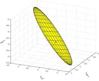
such confidence region is unable to contain the truth. Alternatively, linearly interpolating the

members of the confidence region over finer grid points, the 3 dimensional projection of the

region on the 3 dimensional space of (ξη4,ξη∗,ξη5) does reduce to a thin object too, which

does not contain the truth either. This is illustrated in figure 2.2. The truth is represented by

the red dot which actually is hanging over the flat surface and is outside the region. The 2

di-mensional plane might contain the truth in case the weight of convex combination is so chosen

that 2 dimensional plane passes through the truth, which is a very unlikely expectation. The

simultaneous confidence region might incorporate the sampling variation at the intermediate

(26)

dimension in all the three directions, so that the plane turns into a 3 dimensional solid object

containing the truth(ξη4,ξη∗,ξη5)inside it. The members of the confidence set corresponding

toξη4 andξη5 do incorporate the sampling variation at the two components and hence an

inter-polation method that separately takes into account the sampling variation at that ofξη∗ could

be an option but that is altogether a different problem.

2.2.2 Penalized Empirical Likelihood

2.2.2.1 Formulation

To obtain simultaneous confidence region of functional parameter at finer grid, it is important

to incorporate the variation at the intermediate points of the coarser grid. Since the empirical

likelihood ratio of Hjort et al. (2009) could only allow a very limited refinement of the grid, it

could incorporate variations at only that many chosen points of the functional. To allow

func-tional at finer grid, it is important to surpass the rate p_n=o(n1/3). But the normal calibration of the limit distribution of empirical likelihood as given by Hjort et al. (2009) breaks down

beyond certain growth rate of p_n. We demonstrate this in a simulation study later in section 2.4. Anyway, traditional empirical likelihood does not accommodate faster growth rate of p_n. To attain faster growth rate of p_nit is important to drop the convex hull requirement. With that aim in mind we generalize the penalized empirical likelihood ratio (PELR) for mean functional

of high dimensional data of Lahiri and Mukhopadhyay (2012b) to high dimensional functional

parameterθ(F). The PELR forθ(F)is defined as

RPEL_n (θ(F)) =nnsup πi∈Π

n

∏

i=1

πiexp

−En(θ(F))

such that πi>0, n

∑

i=1

πi=1

(27)

where E_n(θ(F)) = λn∑_kp₌n₁v_k−1 ∑n_i₌₁πigk(Xi,θ(F)) 2

is a distance of the average

estimat-ing functions{g_k(X_i,θ(F)),k=1,2, . . . ,pn}from 0, scaled suitably by the sequence {vk,k= 1,2, . . . ,pn}. The role of the quantityλn=c∗np−1_n is to stabilize the distance and it involves a tuning parameterc∗∈(0,∞). Unlike the traditional empirical likelihood ratio, this formulation

does not require the convex hull requirement because here we do not need to profile the

likeli-hood with respect to the estimating equations separately. Instead, the distance penalty function

E_n(θ(F))takes care of the estimating equations automatically.

2.2.2.2 Limit Distribution

For the asymptotic distribution of RPEL_n (θ(F)) defined in (2.3), we need to introduce some notations at this stage. The estimating functions for the functional parameter θ(F) is dis-cretized at p points in the interval [a,b] and the respective estimating functions are given as {gk(X1,θ(F)),k=1,2, . . . ,p}. We denote the population variance of the estimating functions

by the sequence{σ_k2,k=1,2, . . . ,p}whereVar(g_k(X₁,θ(F)) =σ_k2and the population corre-lation betweeng_j(X₁,θ(F))andgl(X1,θ(F))is denoted asρn(j,l)for 1≤ j,l≤ p. Consider a complete set of orthonormal basis functions{φt,t=1,2, . . .}withφ0= √_b1₋_a of square

inte-grable function spaceL2[a,b], equipped with inner product< f,g>=R

f.gfor f,g∈L2[a,b]. The following assumptions are important in connection to the limit distribution ofRPEL_n (θ(F)).

A1: Max{E σ_k2v−1_k s,k=1, . . . ,p}=O(1)for some givens∈_N.

A2: LimSup_n_→_∞Max{P(g_k(X₁,θ(F)) =x):x∈DX_nk,k=1,2, . . . ,p}<1

whereDX_nk={x∈_R:P(g_k(X₁,θ(F)) =x)>0} fork=1,2, . . . ,p, andn≥1.

A3: Max_j=1,...,pE |gj(X1,θ(F))|q <C for some generic constant C> 0 and some given

(28)

A4: Setg_k(x,θ(F)) =g(x,θ(k_p))and assumeE g(X1,θ(t))

=0 for allt∈[a,b]. Consider

the following conditions.

(1) n−1/2∑n_i=1g(Xi,θ(t))→DW(t),t∈[a,b]whereW is a zero mean Gaussian process

with covarianceρ0(s,t) =E g(X1,θ(s))g(X1,θ(t))

,t ∈[a,b].

(2) G(δ)≡Sup{E g(X1,θ(s))−g(X1,θ(t))2:s,t∈[a,b],|s−t|<δ}whereG(δ)→ 0 asδ →0+ andSup E{g2(X1,θ(s)):s∈[a,b]}<∞.

(3) Define an operatorΓρ0 such thatΓρ0f =∑

∞

k=0γk<φk,f >φk for f ∈L2[a,b]with

∑∞_k₌₀γk<∞(γk≥0 asΓρ0 is non negative definite).

A5: There exists ac∗∈(0,∞)such that 4c∗2R_[₀_,₁_]R_[₀_,₁_]ρ₀2(u,v)dudv<1.

Consider a random process Z(.) which is a zero mean Gaussian process on [0,1] with covariance functionρ0(., .)and subsequently, defineΛ(., .)as

Λ(u,v) =

∞

∑

k=0

c∗k(−2)kρ₀∗(k)(u,v)dudv,

where ρ₀∗(0)(u,v) =1,ρ₁∗(1)(u,v) =ρ0(u,v)

and ρ₀∗(k)(u,v) =

Z

[0,1] . . .

Z

[0,1]

ρ0(u1,u)ρ0(uk,v) k−1

∏

j=1

ρ0(uj,uj+1)du1. . .duk.

Theorem:Undern,p_n→∞, there exists a nondegenrate distribution ofRPEL_n (θ(F))which is given by

−logRPEL_n (θ(F))→Dc∗

Z

[a,b]

Z

[a,b]

(29)

The limit distributions facilitates methods of evaluating approximate confidence region of

θ(F). Letcα be such that

lim n,pn→∞

P

−logRPEL_n (θ(F))≤cα

= (1−α)

then the approximate 100(1−α)% confidence region based onχnforθ(F)is given by

B(χn) =

θ(F)∈Θ:−logR_nPEL(θ(F))≤cα

.

2.2.2.3 Discussion

We revisit the quantile function again to explain how the PELR works. Consider the PELR

based on the estimating equations of the quantile function as given in (2.2). It is possible to

obtain nondegenerate limit distribution of the PELR for arbitrary growth rate of p_n. Hence, now it is possible to find confidence region of the quantile function discretized over much finer

grid. This allows tracking the confidence region of the entire quantile function much accurately.

Consider thepndimensional PELR confidence region of the entire quantile function discretized at finer grid, i.e. of

(ξη1,ξη2,ξη3ξη4,ξη∗,ξη5, . . . ,ηpn).

The finer gridding allows picking quantiles at very fine separation and the PELR does take

into account the sampling variation of quantiles at these finer separations. We pick three grid

points, which are very finely separated. Referring to the discussion made earlier, we can make

the picked grid points as(ξη4,ξη∗,ξη5). Consider the 3 dimensional projection of thepn

dimen-sional PELR confidence region on the space of(ξη4,ξη∗,ξη5), given in figure 2.3. It does

(30)

1.5 2

2.5 3

3.5

2 2.2 2.4 2.6 2.8 3 3.2 3.4 3.6 3.8 2.2 2.4 2.6 2.8 3 3.2 3.4 3.6 3.8 4

ξ_η 4 ξ_η

*

ξ η 5

Figure 2.33 dimensional projection of thepndimensional confidence region on the space of

(31)

at a very fine separation from each other, PELR does provide a meaningful confidence region

containing the truth.

2.2.2.4 On the Cut-off point c_α

It is clearly visible that the limit distribution of RPEL_n (θ(F)) contains unknown population correlation functionρ0, which is not easy to directly estimate. In order to find an approximate

c_α, Lahiri and Mukhopadhyay (2012b) proposed a subsampling method. The method is based on considering subsamples of sizemn(where 1<mn<n) from the sampleχn. The number of such subsamples are way too large and hence the authors proposed to consider only overlapping

subsamples of sizemn. Let the subsamples be denoted byχmln,l=1,2, . . . ,N. Based on these

subsamples, the PELR is evaluated repeatedly to obtain the list{RPELmn ,l(θ(F)),l=1,2, . . . ,N},

where RPEL_m_n ,l(θ(F)) denotes the computed value of PELR after replacing χn by χmln in the

definition of PELR given in (2.3). Finallyc_α is approximated by the subsampling estimatec∗_α given by

N−1 N

∑

l=1

1(−logRPEL_m_n ,l(θ(F))≤c∗_α)≈1−α.

The subsampling sizemnhowever, is a critical issue for the approximation to work. The authors suggested to choosemnsuch thatm−1n +mnn−1=o(1).

2.2.2.5 Constructing Confidence Region

The proposed PELR ratio is a device to evaluate confidence region of the functional

param-eter at finer grids. In the first step, the functional paramparam-eter θ(F) is discretized suitably and expressed in terms of solutions of unboundedly many estimating equations. The second step

(32)

is about aggregating the following collection

B(χn) ={θ(F):−logRPELn (θ(F))≤c∗α}.

Clearly, this is not a point wise confidence region. Construction of a typical point wise

confi-dence region involves first discretizing the functional parameterθ(F), followed by evaluation of point wise confidence intervals based on some cut-off point suitable for the entire

func-tional. Finally the region is obtained by smoothly joining the point wise intervals. However,

here, for the proposed method, it is necessary to pick instances of the discretized version of

the entire functionalθ(F), denoted byθcand(F)at once, which are possible candidates of the regionB(χn). Then we need to check the condition−logRPELn (θcand(F))≤c∗α to conclude on the candidacy ofθcand(F)as a member ofB(χn). Likewise, it is necessary to pick out all such members ofB(χn)to obtain the confidence region. Even for smooth functional parameters like quantile function or probability density function, choosing such candidate curves is not easy.

This is generally because of the unsmooth wiggly nature of the sample versions of theθ(F)of interest. Little notches here and there in the sample version ofθ(F)leads to misleadingB(χn). Two methods, one based on some smooth version of the sample estimate ofθ(F)and the other based on bootstrap resampling are proposed inChapter 3to overcome these issues.

2.3 Applications

In this section we discuss some existing empirical likelihood ratio based confidence region

(33)

2.3.1 Quantile Function for Complete Data

2.3.1.1 Formulation

As mentioned earlier, consider the quantile function defined as

ξ[a,b,F] ={ξη(F),η∈[a,b]⊂[0,1]} where ξη(F) =inf

x {x:F(x)≥η}.

The discretized quantile functionξ[a,b,F]can be represented by the solution of the estimating equations of the form

Z

R

1(X1≤ξηk(F))−ηk

dF=0, where a=η1<η2< . . . <ηp−1<ηpn =b. (2.5)

2.3.1.2 Existing Methods

The traditional empirical likelihood ratio statistic permits a slow growth rate of p_nand hence a coarser discretization of the quantile function than that of the PELR. The traditional empirical

likelihood ratio for quantile function is given by

REL_quant(ξ[a,b,F]) = sup

πi,i=1,2,...,n

n

∏

i=1

nπ_i:πi>0, n

∑

i=1

πi=1,such that n

∑

i=1

πi(1(Xi≤ξηk)−ηk) =0,k=1,2, . . . ,pn,a=η1<η1< . . . <ηpn=b

(2.6)

which has a non degenerate limit distribution for pn=o(n1/3).The 100(1−α)% confidence region based onREL_quant(ξ(a,b,F))is evaluated for a sample χnbased on the limit distribution,

(2p_n)−1/2(−2REL_quant(ξ(a,b,F))−pn)→DN(0,1).

The point wise confidence region of quantile function is somewhat more popular in

(34)

given by Li et al. (1996). The authors considered the data likelihood asL(F) =∏n_i₌₁(F(Xi)− F(Xi−)), the probability of observing the sampleχn. For a fixed quantileξη, the authors con-sidered the nonparametric likelihood ratio as the ratio of the profiled likelihood and the

uncon-strained likelihood as

R(η,t) = supF{L(F):F(t) =η}

sup_F{L(F)} . (2.7)

The point wise confidence region is evaluated based on a cut off point of the limit distribution

of sup_η_∈_[_a_,_b_]|logR(η,t)|which ultimately leads to the confidence region{C(η,rα),η∈[a,b]} given by

C(η,r_α) ={t:R(η,t)≥r_α},

wherer_α =exp(−c2

α(t1,t2)/2). The cutoff pointcα(t1,t2)is the upperα-quantile of

sup t∈[t1,t2]

| B

0₍_t₎

(t(t−1))1/2|

where B0 is a Brownian bridge on [0,1]. The two quantitiest₁ andt₂ are evaluated from the relationst₁=σˆ2(F−1(a))(1+σˆ2(F−1(a)))−1andt2=σˆ2(F−1(b))(1+σˆ2(F−1(b)))−1where

ˆ

σ2(x) = (1−Fn(x))−1Fn(x).

2.3.1.3 PELR Confidence Region

The PELR allows unrestricted refinement of the discretization of the quantile function. The

PELR is given by

RPEL_n (ξ[a,b,F]) =nnsup πi∈Π

n

∏

i=1

πiexp

−E_n(ξ[a,b,F])

such that πi>0, n

∑

i=1

πi=1

(35)

where E_n(ξ[a,b,F]) =λn∑_kp₌n₁v−1_k ∑n_i₌₁πi1(Xi≤ξηk(F))−ηk

2

, scaled suitably by the

se-quence{v_k=ηk(1−ηk),k=1,2, . . . ,pn}. Here the sequence of estimating functions is

{g_k(X₁,ξ[a,b,F]) =1(Xi≤ξηk(F))−ηk,k=1,2, . . . ,pn}.

The confidence region is given by

{B(χn) ={ξ[a,b,F]:−logRPELn (ξ[a,b,F])≤c∗α}.

2.3.2 Quantile Function for Incomplete Data

2.3.2.1 Formulation

Next we consider a situation with incomplete data which is best described by patient survival

data or life time data of products. The study variable of interest corresponding to the individuals

of concern is denoted byX. An observation onX is missing if the trueX_i>C_ifori=1,2, . . .. In that case we only observeC_i’s. However, for each of the individuals, information on some covariate Z is always available. We define a random variable δi, which takes value 1 or 0 according as X_i is observed or not, for i=1,2, . . . ,n. Hence the available information on the experimental units is denoted by

χn={(Y1,Z1),(Y2,Z2), . . . ,(Yn,Zn)}

whereY_i=δiXi+ (1−δi)Ci.We assume that independently and identically distributed random variables X_i’s have common distribution function F. Again, we are interested in the quantile function defined as

(36)

However, for incomplete data the estimating functions {g_k(Y,ξ[a,b,F]),k=1,2, . . . ,pn} are defined differently. For the observations which are non missing, the estimating function is same

as before but for missing observations we need to use the covariate information available on

the corresponding missing experimental units. Fori=1,2, . . . ,nandk=1,2, . . . ,pnwe define the estimating function

g_k(Y_i,Z_i,ξηk)−ηk=gk(δiXi+ (1−δi)Ci,Zi,ξηk)−ηk

= δi1(Xi≤ξηk) + (1−δi)Fˆ(ξηk|Zi)

−η_k.

The quantity ˆF(ξηk|Zi)is a reasonable estimate of the conditional CDF ofX given Zi, which

we fix as

ˆ

F(ξηk|Zi) =P(X ≤ξηk|Zi) =

∑nj=1δj1(Xj≤ξηk)Kh(Zi−Zj)

∑nj=1δjKh(Zi−Zj) .

whereK_h(u) =h−1k(u/h),k(.)being some kernel function andhis the bandwidth.

2.3.2.2 Existing Work

The empirical likelihood based on these estimating equations take the form

REL_quant(ξ[a,b,F]) = sup

πi,i=1,2,...,n

n

∏

i=1

nπ_i:πi>0, n

∑

i=1

πi=1,such that n

∑

i=1

πi( δi1(Xi≤ξηk) + (1−δi)Fˆ(ξηk|Zi)

−ηk) =0,

k=1,2, . . . ,p_n,a=η1<η1< . . . <ηpn =b

.

(2.9)

When it comes to point wise confidence region, formulation of likelihood ratio similar to (2.7)

is provided by Li et al. (1996). Typical to incomplete survival data, the distribution function

F is estimated by the celebrated Kaplan-Meier estimator as ˆF_n(x) =1−∏j:Tj≤x(1−

1

(37)

r_j =∑n_i₌₁1(min{Xi,Zi} ≥ Tj) and T1 <T2 < . . . < TN being the ordered non missing Xi’s. Assuming that quantile confidence region is contained within[T1,TN]the authors proposed the 100(1−α)% confidence region as

{C(η,r_α),η∈[a,b]}={ξη :R(ξη)≥r}

wherer_α =exp(−c2

α(t1,t2)/2),cα(t1,t2)being the upperα-quantile of

sup t∈[t1,t2]

| B

0₍_t₎

(t(t−1))1/2|.

HereB0is the Brownian bridge on[0,1]andt_l’s are defined similarly as in case of quantile for complete data.

2.3.2.3 PELR Confidence Region

The PELR can be constructed by considering (2.3) plugging in

E_n(ξ[a,b,F]) =λn pn

∑

k=1

v−1_k n

∑

i=1

πi1(Xi≤ξηk) + (1−δi)Fˆ(ξηk|Zi)

−ηk

2 ,

scaled suitably by the sequence {vk =n−1∑i=1g2k(i),k=1,2, . . . ,pn} where gk(i) =1(Xi≤

ξηk) + (1−δi)Fˆ(ξηk|Zi)−ηk, fork=1,2. . . ,pnandi=1,2, . . . ,n.

2.4 Simulation Study

In this section we illustrate the asymptotic behavior of the empirical likelihood ratio and we

(38)

2.4.1 Empirical Likelihood in High Dimension

Empirical likelihood ratio has non-degenerate limit distribution for estimating equations of

fixed dimension, given by Qin and Lawless (1994). For fixed number of estimating equations,

say, pof them,−2logREL_n (θ(F))is asymptotically distributed as a chi square distribution with p degrees of freedom. Under growing p= p_n, such that p_n=o(n1/3), −2logREL_n (θ(F))has an asymptotic normal distribution with intact first two moments as it is when p is fixed, i.e.

(2p)−1/2(−2logREL_n (θ(F))−p)→DN(0,1). However, the limit distribution of standard em-pirical likelihood ratio breaks down beyond certain growth rate of pn. Hence, empirical likeli-hood ratio of functional over finer grids does not possess the normal limit distribution beyond

certain grid refinement. In this section we illustrate this behavior of the empirical likelihood

ratio under growing dimension of the estimating equations. For a sequence of independently

and identically distributedp_ndimensional random vectorsX₁,X₂, . . ., we consider the following three data generating models for the illustration. We are particularly interested to investigate the

empirical size of the empirical likelihood ratio tests forH₀:E(X₁) =θ0based on asymptotic

null distribution for different nominal levels under growing p_n.

Model 1: ConsiderW, the Brownian bridge process. Define

X₁= W(0.5

p ),W(

0.5+1

p ), . . . ,W(

p−0.5 p )

.

For testingH₀, we chooseθ0=0, the true mean.

Model 2: Consider U1 as a uniformly distributed random variable on the interval [0,1].

Choose the pdimensional estimating functions

X₁= 1(U₁≤ 0.5

p ),1(U1≤

1+0.5

p ), . . . ,1(U1≤

p−0.5 p )

(39)

We are interested in testing the null hypothesisH₀ choosingθ0as the true mean,

i.e.

θ0= (

0.5 p ,

1+0.5 p , . . . ,

p−0.5 p ). Model 3: ChoosingU1as aBeta(2,4)random variable we fix

X₁= 1(U₁≤0.1+1.0.4

p ),1(U1≤0.1+2. 0.4

p ), . . . ,1(U1≤0.1+p 0.4

p )

and for testingH0, we chooseθ0as

θ0= P(U1≤0.1+

0.4

p ),P(U1≤0.1+2. 0.4

p ), . . . ,P(U1≤0.1+p. 0.4

p )

.

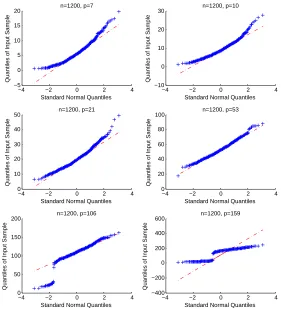
Fixingn=1200, for varying p, the qqplot of the observed empirical likelihood ratio is shown against normal distribution in figure 2.4 for Model 1. Here p is chosen as the largest integer contained in 0.7.n1/3, 1.n1/3, 2.n1/3, 5.n1/3 and 10.n.1/3. For p=106,159, which actually correspond top=5.n1/3andp=10.n.1/3, the empirical distribution of the empirical likelihood ratio deviates significantly from the normal distribution which agrees with the failure of the

asymptotic normal limit of the empirical likelihood ratio beyond certain growth rate of the

dimension.

We test the null hypothesis H₀ at level α =0.05 and 0.10 for all the three models. The difference of the empirical size based on theoretical limit distribution and the nominal size is

reported in table 2.1. We choosen=200,400 and 1200 and pis chosen as the largest integer contained in 0.7.n1/3, 1.n1/3, 2.n1/3, 5.n1/3 and 10.n.1/3. We observe that the difference be-tween nominal size and empirical size increases significantly for p=5.n1/3and p=10.n.1/3 for all the three models. This illustrates the fact that the theoretical nondegenerate limit

(40)

−4 −2 0 2 4 −5 0 5 10 15 20

Standard Normal Quantiles

Quantiles of Input Sample

n=1200, p=7

−4 −2 0 2 4

0 10 20 30 40 50

n=1200, p=21

−4 −2 0 2 4

0 20 40 60 80 100

n=1200, p=53

−4 −2 0 2 4

0 50 100 150 200

n=1200, p=106

−4 −2 0 2 4

−400 −200 0 200 400 600

n=1200, p=159

−4 −2 0 2 4

−10 0 10 20 30

n=1200, p=10

(41)

rate aboveo(n1/3). The simulation study numerically confirms the inadequacy of the empirical likelihood ratio in high dimension and re-inforces the requirement of alternative method in high

dimension which comes in the form of penalized empirical likelihood in the present chapter.

Table 2.1The difference|α−αˆ|of the empirical size ( ˆα) and nominal size (α) of the empirical

likeli-hood ratio test forH₀based onN=500 replications for varying values ofnandp.

n=200 n=400 n=1200

α α α

Model p_n p 0.05 0.10 p 0.05 0.10 p 0.05 0.10

Model 1 0.7n1/3 4 0.016 0.048 5 0.006 0.028 7 0.016 0.036 1.n1/3 5 0.020 0.052 7 0.012 0.040 10 0.002 0.031 2.n1/3 11 0.016 0.008 14 0.015 0.005 21 0.004 0.002 5.n1/3 29 0.165 0.120 36 0.028 0.026 53 0.022 0.018 10.n1/3 58 0.555 0.518 73 0.198 0.220 106 0.070 0.088 Model 2 0.7n1/3 4 0.038 0.018 5 0.016 0.014 7 0.018 0.004 1.n1/3 5 0.028 0.017 7 0.026 0.012 10 0.014 0.002 2.n1/3 11 0.184 0.164 14 0.056 0.036 21 0.016 0.014 5.n1/3 29 0.505 0.412 36 0.292 0.250 53 0.088 0.076 10.n1/3 58 0.915 0.820 73 0.717 0.626 106 0.334 0.288 Model 2 0.7n1/3 4 0.004 0.012 5 0.002 0.020 7 0.000 0.002 1.n1/3 5 0.004 0.002 7 0.014 0.012 10 0.000 0.003 2.n1/3 11 0.030 0.016 14 0.020 0.016 21 0.014 0.008 5.n1/3 29 0.142 0.092 36 0.040 0.086 53 0.012 0.034 8.n1/3 46 0.814 0.764 58 0.298 0.248 85 0.038 0.080

2.4.2 Numerical Performance of PELR

In this subsection we study the numerical performances of the proposed PELR confidence

region for quantile function separately for complete data and incomplete data. We compare

the proposed PELR confidence region with that of the based on empirical likelihood without

(42)

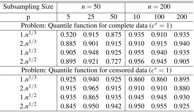
Table 2.2Coverage accuracy of the confidence regions for the subsampling based cut-off points of limit distribution of PEL under various subsampling size where desired coverage accuracy is 0.90

Subsampling Size n=50 n=200

p 5 25 50 10 100 200

Problem: Quantile function for complete data (c∗=1) 1.n1/3 0.520 0.915 0.875 0.935 0.910 0.935 2.n1/3 0.885 0.901 0.915 0.910 0.915 0.940 1.n1/2 0.905 0.948 0.925 0.955 0.940 0.935 2.n1/2 0.895 0.921 0.727 0.956 0.945 0.905

Problem: Quantile function for censored data (c∗=1) 1.n1/3 0.925 0.940 0.925 0.860 0.860 0.895 2.n1/3 0.915 0.965 0.915 0.910 0.910 0.880 1.n1/2 0.935 0.865 0.935 0.945 0.945 0.930 2.n1/2 0.845 0.950 0.942 0.950 0.955 0.925

2.4.2.1 Quantile Function for Complete Data

For confidence region of quantile function corresponding to complete data, we consider

sam-ples of sizenfrom the standard exponential distribution with mean 1, and evaluate confidence regions for

ξ[0.70,0.95,F] ={ξη,η ∈[0.7,0.95]}.

We choose n=50 and 200 and pn as the largest integers contained in 0.7.n1/2,n/2 andn. The related results on coverage accuracy and average length are given in table 2.3.

2.4.2.2 Quantile Function for Incomplete Data

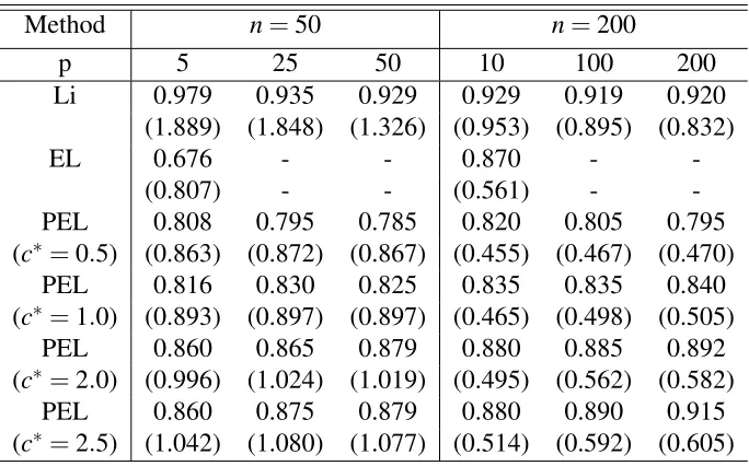
For confidence region of quantile function corresponding to incomplete data, we generate the

(43)

Table 2.3Coverage accuracy and average length of the estimated confidence region for the quantile function when the nominal coverage level is 0.90

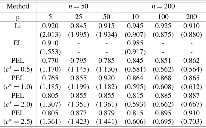
Method n=50 n=200

p 5 25 50 10 100 200

Li 0.920 0.845 0.915 0.945 0.925 0.910

(2.013) (1.995) (1.934) (0.907) (0.875) (0.880)

EL 0.910 - - 0.985 -

-(1.553) - - (0.917) -

-PEL 0.770 0.795 0.785 0.845 0.851 0.862

(c∗=0.5) (1.170) (1.145) (1.130) (0.581) (0.562) (0.564)

PEL 0.765 0.855 0.920 0.864 0.868 0.865

(c∗=1.0) (1.185) (1.199) (1.182) (0.595) (0.608) (0.612)

PEL 0.805 0.855 0.855 0.815 0.885 0.887

(c∗=2.0) (1.307) (1.351) (1.361) (0.593) (0.662) (0.667)

PEL 0.805 0.877 0.879 0.815 0.895 0.910

(c∗=2.5) (1.361) (1.423) (1.441) (0.606) (0.695) (0.703)

wherep_i= exp(1+0.25Zi)

1+exp(1+0.25Zi). This leads to approximately 25% to 30% missing data. We evaluate

confidence regions for

ξ[0.70,0.95,F] ={ξη,η ∈[0.7,0.95]}.

We choose n=50 and 200 and p_n as the largest integers contained in 0.7.n1/2,n/2 andn. The related results on coverage accuracy and average length are given in table 2.4.

2.4.2.3 Subsampling Based Calibration

First of all, we need to calculate approximate cut off point for the limit distribution of PELR.

We choose appropriate subsampling size to implement the subsampling method suggested by

Lahiri and Mukhopadhyay (2012b). The subsamples are taken to be overlapping blocks of sizes

(44)

Table 2.4Coverage accuracy and average length of the estimated confidence region for the quantile function corresponding to incomplete data when the nominal coverage level is 0.90

Method n=50 n=200

p 5 25 50 10 100 200

Li 0.979 0.935 0.929 0.929 0.919 0.920

(1.889) (1.848) (1.326) (0.953) (0.895) (0.832)

EL 0.676 - - 0.870 -

-(0.807) - - (0.561) -

-PEL 0.808 0.795 0.785 0.820 0.805 0.795

(c∗=0.5) (0.863) (0.872) (0.867) (0.455) (0.467) (0.470)

PEL 0.816 0.830 0.825 0.835 0.835 0.840

(c∗=1.0) (0.893) (0.897) (0.897) (0.465) (0.498) (0.505)

PEL 0.860 0.865 0.879 0.880 0.885 0.892

(c∗=2.0) (0.996) (1.024) (1.019) (0.495) (0.562) (0.582)

PEL 0.860 0.875 0.879 0.880 0.890 0.915

(c∗=2.5) (1.042) (1.080) (1.077) (0.514) (0.592) (0.605)

of Lahiri and Mukhopadhyay (2012b): m−1_n +m_nn−1 =o(1). Considering 500 Monte Carlo replications, and comparing the nominal level of 0.90 to the proportion of replications which

results in acceptance of the true value of the functional inside the region, we decide on the

cutoff points. The results related to the subsampling method for various selections of m_n are given in table 2.2. From these simulation studies subsampling size mn =2n1/3 seems quite adequate for good enough coverage accuracy. We continue the rest of the simulation study on

band length and coverage accuracy with this subsample size to get the necessary cut off points

for different cases.

The confidence region based on empirical likelihood method without penalization is

de-noted by EL. This is obtainable only for p_n=o(n1/2), hence we report results corresponding to EL only for p_n =0.7.n1/2. However, the point wise confidence region given by Li et al. (1996) and denoted by Li and PELR confidence region work for faster rates, i.e., for each of

(45)

2.4.2.4 Findings

The coverage accuracies of the estimated confidence regions are reported along with average

width of the confidence regions with in parentheses in table 2.3 and 2.4. For fixedc∗, with in-crease in sample sizen, average width decreases. However, for fixed sample size, with increase in value of the tuning parameterc∗, average width and coverage proportion are increasing. It is recommended to tunec∗ such that at that tuned value, the coverage proportion is closest to the desired level of 0.90. EL works only for very coarse gridding of the quantile function and hence the confidence region of the quantile function fails to give information on the quantiles

at finer separations. So, it should be kept in mind that for EL, the reported coverage accuracy,

however accurate that may be, is only relevant to the quantiles at the course discretization. The

other two methods, however, work for arbitrarily fine discretization of the quantile function

and is way more informative than EL. The larger the value of p_n the better is the coverage accuracy, which is somewhat expected as larger p_nleads to finer discretization of the quantile function. Point wise confidence region proposed by Li et al. (1996), denoted by Li gives much

wider confidence regions than that of PEL and also gives somewhat over coverage, whereas

PEL method gives little under coverage. However tuning the parameter c∗, the under cover-age of PEL can be improved considerably. The under covercover-age of the PEL method is actually

attributed to the region construction algorithm and can be resolved considerably by bootstrap

(46)

2.5 Proof of the Theorem

To prove the theorem given in 2.4 we need to verify the conditions of Lahiri and Mukhopadhyay

(2012b).

First considering condition(ii)of C.3 of Lahiri and Mukhopadhyay (2012b) for

max{|h1|,|h2|}<δ where δ >0,

≤E|g(X₁,θ(u+h1)){g(X1,θ(v+h2))−g(X1,θ(v))}|

+E|{g(X₁,θ(u+h1))−g(X1,θ(u))}g(X1,θ(v))|

≤2Sup{E g(X₁,θ(u))2:u∈[a,b]}1/2

Sup{(E|g(X₁,θ(u+t))−g(X1,θ(u))|2)1/2:u∈[a,b],|t| ≤δ}

Hence, from assumption(2)ofA4,|ρ0(u+h1,v+h2)−ρ0(u,v)| ≤K.G(δ), for some constant

0<K<∞.

Withh(u,v) =K,

∞

∑

k=0

<|φ_k|,|Γ_hφ_k|>=

∞

∑

k=0

<|φ_k|,|

Z

Kφ_k|>

=K<|φ₀|,

Z

|φ₀|>+K

∞

∑

k=1

<|φ_k|,|

Z

φk|>

=K(

Z

(47)

Now considering condition (iii) of C.3 of Lahiri and Mukhopadhyay (2012b), from as-sumption(3)ofA4,

∞

∑

k=0

<φk,Γρ0φk>

∞

∑

k=0

<φ_k,γ_kφ_k>

= ∞

∑

k=0

γk<∞

Finally, for condition(i)of C.3 of Lahiri and Mukhopadhyay (2012b),

Z

[a,b]

Z

[a,b]

ρ₀2(u,v)dudv=

∞

∑

k=0

γ_k2<(4c∗2)−1

⇔4c∗2

Z

[a,b]

Z

[a,b]

ρ₀2(u,v)dudv<1

Forθ(F) =ξ[a,b,F], the quantile function,ρ0(s,t) =s∧t−st. Note that

Z

[a,b]

Z

[a,b]ρ

2

0(s,t)dsdt

=

Z

[a,b]

Z

[a,b]

(s∧t)2dsdt−(

Z

[a,b] s2ds)2

=2

Z

[a,b]

Z

[a,t]

s2dsdt− _s3 3 p b a 2 = 2 3 Z

[a,b]

(t3−a3)dt−

(b3−a3)

3

2

= 1

6(b

4₋_a4₎₋2

3 a

3₍_b₋_a₎ −

(b3−a3)

3

2

Hencec∗∈

0,0.51₆(b4−a4)−2 3 a

3₍_b₋_a₎ −

(b3−a3)

3

2 −1/2

(48)

Chapter 3 Evaluation of Confidence Region of High

Dimensional Functional Parameter

3.1 Introduction

Nonparametric confidence region for functional parameters is explored quite extensively by

researchers over the years. The focus of those works has been primarily to propose a suitable

pivot or statistic, followed by its sampling distribution and finally a suitable cut-off point.

However, not much light is thrown on the practical difficulties in connection to construction of

the confidence region. In fact, for certain functional parameters, due to the sheer computation

time and related complexity, the coverage accuracy of the proposed confidence regions are

seldom discussed. In many situations, in spite of having a well documented confidence region

evaluation method, difficulties are often encountered to practically implement them and their

accuracy is often questionable.

Sometimes the computational complexity can be somehow resolved with the aid of modern

(49)

popu-lation functionals such as the quantile function, regression function or the probability density

function, general shape of the functional becomes critical. In some situations, we may need

the entire curve of high dimensional functional at a time to check the criteria for its candidacy

of the confidence region. In such cases, it often becomes very important to correctly identify

the general shape and some critical features of the functional with some acceptable accuracy.

Else the estimated region may completely fall apart, however sophisticated the pivot or statistic

may be. In this chapter we try to bring in certain such practical difficulties in connection to

evaluation of confidence region of such high dimensional functional parameters and propose

two methods to overcome the difficulties.

SupposeX1,X2, . . .be a sequence of independently and identically distributed random

vari-ables with common probability distribution functionF. We observe a random sample of sizen which can be denoted by

χn={X1,X2, . . . ,Xn}.

A functional parameter of the unknown parent population F is given by θ(F) which can be vector valued. When θ(F) is finite dimensional, i.e. for some integer p, if θ(F)∈Θ⊂_Rp,

confidence region of θ(F) is generally evaluated by grid search method in the correspond-ing finite dimensional space Θ. For example, suppose we are considering confidence region

of θ(F) = (θ1(F),θ2(F))0, where θ1(F) =R_RX1dF andθ2(F) = R_RX₁2dF, the first two raw

moments ofF. For the ease of discussion we confine ourselves in only likelihood based con-fidence region where the data likelihood ratio is denoted by R_n(F). The confidence region

of θ(F) = (θ1(F),θ2(F))0 is evaluated by varying θ(F) over some suitably chosen grids in

Θ= (−∞,∞)×[0,∞)and collecting

High Dimensional Methods in Statistics, Data Mining and Finance.

ABSTRACT

DEDICATION

BIOGRAPHY

ACKNOWLEDGEMENTS

TABLE OF CONTENTS

LIST OF TABLES

LIST OF FIGURES

Chapter 1

Introduction

Chapter 2

Empirical Likelihood Method for High

Dimensional Functional Parameters

2.1

Introduction

∏

∑

∏

∑

∑

2.2

High Dimensional Functional Parameters

2.2.1

Motivation

2.2.2

Penalized Empirical Likelihood

∏

∑

∑

∏

∑

2.3

Applications

2.3.1

Quantile Function for Complete Data

∏

∑

∑

∏

∑

2.3.2

Quantile Function for Incomplete Data

∏

∑

∑

∑

∑

2.4

Simulation Study

2.4.1

Empirical Likelihood in High Dimension

2.4.2

Numerical Performance of PELR

2.5

Proof of the Theorem

∑

∑

∑

∑

∑

∑

∑

Chapter 3

Evaluation of Confidence Region of High

Dimensional Functional Parameter

3.1

Introduction

_∏