Information and Software Technology

(1)

An approach to identifying causes of implied scenarios using unenforceable orders

In-Gwon Song

⇑

, Sang-Uk Jeon, Ah-Rim Han, Doo-Hwan Bae

Department of Computer Science, College of Information Science and Technology, KAIST, Daejeon, Republic of Korea

a r t i c l e

i n f o

Article history:

Available online 24 November 2010 Keywords:

UML 2.0

Interaction overview diagram Sequence diagram

Scenarios

Requirements veriﬁcation Implied scenarios

a b s t r a c t

Context: The implied scenarios are unexpected behaviors in the scenario speciﬁcations. Detecting and handling them is essential for the correctness of the scenario speciﬁcations. To handle such implied sce-narios, identifying the causes of implied scenarios is also essential. Most recent researches focus on detecting those implied scenarios, themselves or limited causes of implied scenarios.

Objective:The purpose of this research is to provide an approach to detecting the causes of implied sce-narios.

Method:The scenario specification is a set of events and a set of relative orders between the events, and enforces them for its implementation. Among the orders, a set of orders that cannot be inherently enforced is the unenforceable orders. Obviously, existence of unenforceable orders leads the implied sce-narios. To obtain the unenforceable orders, we first provide a method to represent each of the specifica-tion and its implementaspecifica-tion as a set of orders between events, called the causal order graph. Then, the differences between them are the unenforceable orders.

Results: Because the unenforceable orders consist of events and their order relation that are specified in the scenario specification, they can point out which part of the scenario specification should be consid-ered to handle the implied scenarios. In addition, our approach supports the synchronous, asynchronous, and FIFO communication styles without the state explosion or heavy computational overhead. To validate our approach, we provide two case studies.

Conclusion:This approach helps a designer to effectively correct the scenario speciﬁcation by identifying where to be ﬁxed, especially in large cases and under the various communication styles.

1. Introduction

Since the requirements specification determines the scope of subsequent development phases, its correctness is important. As scenarios become popular as a means of specifying the require-ments[13], Message Sequence Charts (MSCs)[8]or Unified Model-ing Language (UML)[12]interaction diagrams are widely used for the scenario descriptions because of their proper formality and ease of use. However, the scenario specification specified in the MSCs or UML interaction diagrams may cause differences between the specification and its implementation: the scenario specification can describe only partial behaviors of a system, while its imple-mentation has full behaviors. Such differences are referred to as the implied scenarios[2,15]. More formally, the implied scenarios are differences between a scenario specification and its minimal implementation[15,11], which satisfies the scenario specification. In this paper, we refer to the minimal implementation as imple-mentation model. Note that the implementation model is not the source code, but a smallest set of behaviors satisfying the

specifica-tion. Therefore, the implied scenarios means inherent but unex-pected behaviors, and they should be identified to obtain the correct scenario specification.

Several works have been proposed to detect the implied scenar-ios[9,11,15]. In these approaches, the model-checking technique is used through the synthesis of an automata-based implementation model. Such approaches have two limitations. First, the model-checking technique can only identify implied scenarios as a form of error traces. Such error traces do not indicate the locations in the scenarios specification where the designer should consider to handle the implied scenarios. We refer to such locations as the causes of implied scenarios. With the knowledge of the causes of plied scenarios, it certainly becomes more easier to handle the im-plied scenarios. Moreover, automatic identification of the causes enables (semi-)automatic treatment of the implied scenarios. Another limitation is that they assume only the synchronous communication style in the scenario specification. This is because handling the asynchronous communication style may lead to the state explosion in the synthesis of the automata-based implemen-tation model. However, emerging software, such as web services and embedded software, requires the asynchronous communica-tion style. Therefore, in the deteccommunica-tion of the implied scenarios,

⇑Corresponding author. Tel.: +82 423507739; fax: +82 423508488. E-mail address:[email protected](I.-G. Song).

Contents lists available atScienceDirect

Information and Software Technology

(2)

the consideration of the asynchronous communication style as well as the synchronous one is needed.

To address those limitations, in this paper, we provide an ap-proach to detecting unenforceable orders to identify causes of im-plied scenarios. Essentially, the scenario speciﬁcation enforces relative orders between events. If some orders among them cannot be enforced in an implementation, such orders cause implied sce-narios. We call such orders theunenforceable orders. (We will give more detailed explanation on them in Section5.1.) To detect the unenforceable orders, our approach creates a graph that represents the orders enforced by the scenario speciﬁcation. Based on the graph, we also construct another graph representing the orders that are enforceable in the implementation model. Then, we calcu-late differences between those graphs. These represent the unen-forceable orders.

Our approach has the following advantages:

Since the unenforceable orders correspond to the events of the scenario speciﬁcation, they can be used as the causes of implied scenarios, which indicate which part of the scenario speciﬁcation should be considered to handle the implied scenarios.

As our approach does not synthesize any automata-based

model, it can handle the asynchronous communication without producing the state explosion. Based on the asynchronous communication, our approach can also handle the various com-munication styles, including the synchronous and FIFO commu-nication style.

Since the two graphs are based on the scenario speciﬁcation and its implementation model, not only are the implied scenarios caused by the non-local choice detected, but also the input–out-put implied scenarios.

Our approach provides the ﬁne-grained detection because we separately use the sending and receiving events unlike previous approaches[9,11,15].

Our approach is applicable for the large-scale scenario speciﬁca-tion because the complexity of our algorithm isO(jVspecj3) where Vspecis a set of events in the scenario speciﬁcation.

The rest of this paper is organized as follows: In Section2, we discuss related works. Section 3defines several terms and con-cepts. In Section4, we explain the loop unrolling to deal with loops in the scenario specification. Section5defines the unenforceable orders, and presents the algorithms. In addition, the complexity of the algorithms is shown in order to show the efficiency of our approach. In Section6, we present a technique to support loops and other communication styles. After presenting two case studies in Section7, we conclude our approach with the discussion of fu-ture work in Section8.

2. Related work

The term ‘‘implied scenario’’ was ﬁrst introduced by Alur et al.

[2]. They provided a framework to verify that a given scenario specification is realizable with some implementation. Their realiz-ability is classified on two levels: weak and strong. The weak real-izability is satisfied if a scenario specification has all the combinations of the local behavior of each process, while the strong realizability is satisfied if a scenario specification satisfies the weak realizability and if it is deadlock-free. If those realizabil-ities are not satisfied, the scenario specification has the implied scenarios. Their work focuses on determining whether a scenario specification has implied scenarios or not, and is limited to the specifications that specify finite system behaviors, which means that no loop is allowed in the specification.

Uchitel et al. provided the method and tool for detecting im-plied scenarios[15]. Their method can deal with inﬁnite system behaviors which are expressed by loops of an high-level message sequence chart (hMSC). They presented an algorithm that builds the Labeled Transition System (LTS) behavior model as the implementation model. They also presented the way of obtaining differences between the MSC speciﬁcation and its implementa-tion model. Since they use the model-checking technique to ob-tain the differences, their algorithm can produce the implied scenarios in the form of error traces, so that their work cannot identify the causes of implied scenarios. In addition, their work is applicable only to the synchronous communication style and assumes the synchrony hypothesis, which means that there are no events between sending and receiving events of a message.

Letier et al. have extended Uchitel et al.’s work by considering an observation that the reception of a message cannot be con-trolled, but is monitored[9]. They refer to the implied scenarios, resulting from their approach, as the input–output implied scenar-ios. Their work still assumes the synchronous communication and synchrony hypothesis.

Muccini proposed another approach to detecting implied sce-narios, not involving the use of the model-checking technique. In-stead, it starts from the detection of the non-local choices. Then, by investigating the events occurring after the non-local choices, it detects the implied scenarios. Although this approach is not aimed at detecting the causes of implied scenarios, it can be used to identify which choices are problematic through the intermediate results. However, this approach does not touch upon the input– output implied scenarios and assume the synchronous communi-cation and synchrony hypothesis.

Baker et al. proposed an approach to detecting and resolving semantic pathologies in UML sequence diagrams[5]. Based on a graph, which is generated from the UML sequence diagram and referred to as the causal order graph, they proposed the condi-tions for detecting the pathologies. The approach supports various communication styles. However, their work has three limitations. First, the approach cannot be used when the scenario speciﬁca-tion has loops. Second, since the approach does not consider the state-merging effects, the detected pathologies may omit some implied scenarios. Third, the synchrony hypothesis is par-tially assumed.

Recently, in the service-oriented architecture area, several re-searches for detecting the implied scenarios were presented as a name of ‘‘check of local enforceability’’ [7,19]. However, those works only check whether the implied scenarios exist or not, like Alur et al.’s work[2].

3. Background

3.1. UML scenario speciﬁcation

Our approach uses the scenario specification that is represented as UML interaction diagrams. We refer to it as theUML scenario specification. Since it has similar structures with the MSC scenario specification in[15], their formal definitions are nearly the same. In spite of that, we reformulate our UML scenario specification to clearly describe our approach. Our UML scenario specification con-sists of basic sequence diagrams (bSDs) and a basic interaction overview diagram (bIOD) which are simplified from original se-quence diagrams and an interaction overview diagram in UML 2.0, respectively.

Deﬁnition 1. A basic sequence diagram B is a structure (O,M,L,loc, <), where:

(3)

O is a set of event occurrences. It consists of a set of sending occurrencesSand a set of receiving occurrencesR.

Mis a set of messages. A messagemis a structure (s,r,n) such thats2 S;r2 Randnis the label of the message. In addition, we denote a labeling functionlblsuch thatlbl(s) =lbl(r) =nfor (s,r,n)2M.

Lis a set of lifelines.

loc:O?Lmaps an event occurrence to a lifeline.loc1₍_l_{) is a set} of event occurrences on a lifelinel.

< is a set of total orders <l #loc1(l)loc1(l) between event occurrences. The orders depict an order relationship between two adjacent event occurrences.

Definition 2. The basic interaction overview diagramIis a graph (E,V), whereVis a set of vertices that consist of control vertices and vertices referencing bSDs, andE#(VV) is a set of directed edges that represent control flows. The control vertices are catego-rized intoinitial,final,decision, andmerge.

Sequence diagrams in UML 2.0 have combined fragments to de-scribe control structures or provide restricted views. We omit the combined fragments in the deﬁnition of the bSD because such con-trol structures can also be represented by concon-trol vertices of the bIOD, and the restricted views do not affect behaviors presented by the bSD.

A bIOD provides a means of describing control flows between bSDs. It is a graph that consists of the vertices referencing bSDs, control vertices, and edges representing the control flows between the vertices. The control vertices consists ofinitial,final,decision, andmerge. In this paper, we do not use the fork and merge nodes. While the different lifelines may concurrently behave, those nodes may introduce another parallelism. There are no exact definitions of its semantics. To deal with those parallelisms, we should first define their formal semantics. Since that task is not within the scope of this paper, we assume that the fork and merge nodes are not used in our scenario specification. We also assume that there is only one initial vertex for simplicity.

Now we define the UML scenario specification. It consists of a set of bSDs, a bIOD, and reference relationships between them. The definition of a UML scenario specification is as follows:

Deﬁnition 3. A UML scenario speciﬁcation is a structureðB;I;refÞ, whereBis a set of bSDs,Iis a bIOD, andrefis a mapping function from a referencing vertex inIto a referenced bSD inB.

3.2. Causal order graph

The UML sequence diagram describes the sending and receiving events of the messages, and the orders between them. Those events and orders can be formalized as a partially ordered set. To represent the partially ordered set, many prior works use a direc-ted graph. The graph is referred to as thecausal order graph. In the causal order graph, each vertex represents the sending or receiving event in the sequence diagram, and each edge indicates that the event that corresponds to its target vertex should occur after the occurrence of the event that corresponds to its source vertex.

Fig. 1shows an example bSD and its causal order graph. For a clear explanation, we denote the sending event and receiving event of a message assnandrn, respectively, wherenis an identiﬁer for each message. In Fig. 1a, the events s1 and r1 are sending and receiving events for the message ‘‘questionnaire’’, respectively. Since a sending event should occur before its corresponding receiving event, the causal order graph has an edge froms1tor1as shown inFig. 1b. The events1is located in a place above the events2in

Fig. 1a. According to the semantics of the sequence diagram, this

means that the event s2 should arise after the events1. Hence, the causal order graph has an edge from the events1to the event s2. In this way, a causal order graph for a sequence diagram can be obtained. Its formal deﬁnition is as follows:

Deﬁnition 4.A causal order graph is deﬁned as a directed graph G ¼ ðE;VÞ.V represents the set of vertices that represent events, whileE#VV represents a set of edges which denote orders between vertices.

4. Loop unrolling

When a system is described by the causal order graph and it has loops, the causal order graph also has loops. However, since the loops in the causal order graph represent concurrent events, the causal order graph is not appropriate for representing the UML sce-nario speciﬁcation with loops. Therefore, we devised a loop-unroll-ing technique.

The basic idea for the loop-unrolling technique is as follows. Let’s assume that the bSDbhas an unenforceable order andbis in a loop. After the loop is unrolled, the bSDbstill has the unen-forceable order.

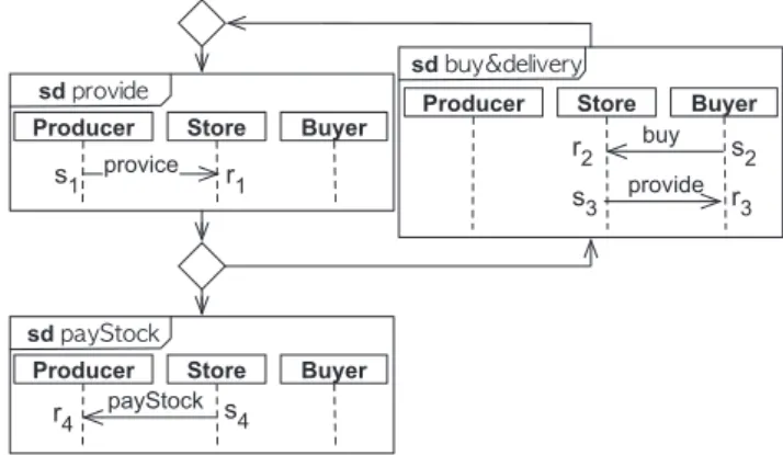
In addition to the basic idea, we need to consider the concatena-tions between bSDs since the concatenaconcatena-tions introduce another causal order relationship. For example, inFig. 2, an events4 in the bSD ‘‘payStock’’ should happen after an eventr1 of the bSD ‘‘provide’’ because the bSD ‘‘payStock’’ is one of the next bSD of the bSD ‘‘provide’’ ands4andr1are on the same lifeline: the order ‘‘r1tos4’’ is enforced. In order to prevent loss of such orders, we need to conserve them after the loop unrolling.

With this idea, we devise transformation templates of a generic loop as shown inFig. 3.Fig. 3a shows the generic loop of the bIOD. Each circle means a subgraph of the bIOD. To make it as a simpler form, it is re-arranged as shown inFig. 3b. Then, the re-arranged loop is unrolled as shown inFig. 3c.

Before justifying our unrolling technique, let’s deﬁne the causal-ity relationee0 _{which means that the event} _e_{should happen}

Producer Store questionnaire advertise put s₁ r₁ s₂ r₃ s₃ r₂ Consumer get r₄ s₄ r₁ s₂ s₁ r₂ r₃ s₃ s₄ r₄

(a) Example bSD (b) Causal order graph of (a) Fig. 1.Example of the causal order graph.

sd

Producer Store Buyer provice

s₁ r₁

sd

Producer Store Buyer payStock _s

4

r₄

sd

Producer Store Buyer buy provide

r₂

s₃ r₃

s₂

(4)

beforee0_{. Note that the causality relation}_{has the same semantics}

with the causal order graph.

Now, we can show the validity of our unrolling technique with a simple argument. First, sinceFig. 3c has all the bSDs inFig. 3a, cau-sality relations in each bSD are obviously preserved after the loop unrolling. LeteA,eB,eC, andeDbe events that are arbitrarily selected from A, B, C, and D inFig. 3, respectively. Then,Fig. 3a directly shows the causality relationseAeB,eBeD,eBeC, andeCeB. By the transitiveness of the causality relation, the relationseAeB, eAeC,eAeD,eBeB,eBeC,eBeD,eCeB,eC eC, andeCeD are inferred. These causality relations are preserved in Fig. 3c. Therefore,Fig. 3c conserves all causality relations ofFig. 3a. This means that all orders that are enforced by an original UML scenario speciﬁcation are preserved in the unrolled UML scenario speciﬁca-tion. In addition, sinceFig. 3a is a generic loop, our loop unrolling can be applied to all cases.

The form for the unrolled loop, shown inFig. 3c, has more in-stances of ‘‘B’’ and ‘‘C’’ than the original one. For the optimization of our approach, we devised several techniques to reduce them. However, since the optimization is not in the scope of this paper, we will not describe them.

5. Detecting unenforceable orders

The unenforceable orders are relative orders that are enforced by the scenario specification, but cannot be enforced when the specification is implemented. Obviously, if they exist in a scenario specification, the implied scenarios also exist. Since they consist of the events that are specified in the scenario specification, they can be pointed out in the scenario specification itself. Therefore, the unenforceable orders can be used to identify the causes of implied scenarios. In our approach, the unenforceable orders are obtained by differentiation between two causal order graphs representing the scenario specification and its implementation model. We refer to the two causal order graphs as thespecification order graphand theimplementation order graph, respectively.

Now we brieﬂy illustrate our idea of detecting the unenforce-able orders with an example shown inFig. 4. InFig. 4a, the object ‘‘Producer’’ should send the message ‘‘provide’’ to the object ‘‘Store’’ before the object ‘‘Buyer’’ sends the message ‘‘buy’’. The ‘‘Buyer’’ can-not know whether the ‘‘Producer’’ already sent the message ‘‘ pro-vide’’ or not. Thus, the ‘‘Buyer’’ may send the message ‘‘buy’’ before the message ‘‘provide’’ is sent. By this reasoning, we can come up with an implied scenario as shown inFig. 4b. This reasoning shows

another fact: the order ‘‘r1tor2’’ is defined in the scenario specifi-cation, but not held in the implementation model. It means that the order ‘‘r1 to r2’’ is included in specification order graph, but not in theimplementation order graph. According to the above def-inition, the order ‘‘r1tor2’’ is an unenforceable order.

If the order can be enforced by introducing additional mecha-nisms, such as the coordinator, the implied scenario shown in

Fig. 4b is also removed. Therefore, we can regard the unenforceable order ‘‘r1tor2’’ as a cause of implied scenarios.

Fig. 5illustrates the overview of our approach. Our approach consists of the following steps: (1) From the UML scenario specifi-cation unrolled by our loop-unrolling technique, the specifispecifi-cation order graph is obtained. (2) Then, the implementation order graph is obtained by manipulating the specification order graph. (3) Fi-nally, the differences between the specification order graph and

A B C D A B D C B B C A B D B C

(a) Generic loop (b) Re-arrangement as a simpler form (c) Unrolled loop : decision/merge vertex : subgraph of the bIOD

Fig. 3.Unrolling of generic loop.

Producer Store Buyer provide buy payStock provide s₁ r₁ s₄ r₄ r₂ s₃ r₃ s₂

Producer Store Buyer

provide buy payStock provide s₁ r₁ s₄ r₄ r₂ s₃ r₃ s₂

(a) Given scenario (b) Implied scenario of (a) Fig. 4.Example bSD and its implied scenario.

UML scenario specification

Extracting a causal order graph from the speci cation

Creating a causal order graph as an implementation model

Implementation order graph Specification order graph

Calculating differences

Unenforceable orders

(5)

implementation order graph are calculated. For simplicity, in this section, we consider only the asynchronous communication style. The FIFO and synchronous communication styles will be covered in Section6.

Now, according to the overview, we first define the enforceable orders with the definitions of the specification and implementation order graph in Section5.1. Then, to show the efficiency of our ap-proach, the algorithms for detecting the enforceable orders will be shown in Section5.2.

5.1. Deﬁnitions

5.1.1. Speciﬁcation order graph

The specification order graph represents order relationships specified in the scenario specification. Since the UML scenario specification consists of bSDs and a bIOD, we first describe the definition of the specification order graph of a bSD. Then, we define the specification order graph of the whole UML scenario specification.

In Section3, we brieﬂy illustrated the causal order graph of the bSD. Now, we provide its formal deﬁnition.

Deﬁnition 5. The speciﬁcation order graph gB

spec of a bSD

B= (O,M,L,loc,<) is deﬁned as follows:

gB

spec¼ ðfðb;eÞjðb;eÞ 2<l;8l2Lg [ fðs;rÞjðs;rÞ 2Mg;OÞ

Fig. 6shows a UML scenario specification of a small delivery system. The lower parts ofFig. 6, ‘‘sddeliveryA’’ and ‘‘sddeliveryB’’, are borrowed from Letier et al.’s work [9]. To effectively show our approach, we extend the example. The scenario specification inFig. 6describes the procedure of product sales with three bSDs and one bIOD. When the scenario begins, the delivery department transmits an order to the factory to produce a product. Then, the client requests a product from the seller with the type of the prod-uct. The seller who receives the request from the client transmits the request to the delivery department. Finally, the delivery department sends the requested product to the client. The specifi-cation order graphs for the bSDs inFig. 6are shown inFig. 7.

Through the composition of the specification order graphs of bSDs, we can define the specification order graph for the entire sce-nario specification. We first define the composition operator

be-tween two bSDs. Then, by using it, the definition of the specification order graph for the entire scenario specification will be given. There are two kinds of composition: the asynchronous concatenation and synchronous concatenation[4]. The synchro-nous concatenation assumes the synchronization scheme, such as a coordinator or mutex, while the asynchronous concatenation does not. In this paper, the asynchronous concatenation is only used because we do not assume such a synchronization scheme. In the asynchronous concatenation, each lifeline is independently composed. To formalize the asynchronous concatenation, we de-vise an asynchronous concatenation operator. Thesequentially concatenates causal order graphs of two bSDs in an asynchronous manner. According to the definition of asynchronous concatena-tion[4], ifg1g2is given and theg1andg2are causal order graphs, the asynchronous concatenation operator creates a new edge that connects the last event ofg1to the first event ofg2in each lifeline.

Deﬁnition 6. Asynchronous concatenation operator for the causal order graphsgB1_and_gB2_{is deﬁned as follows:}

gB1gB2_¼gB1_[gB2_{[ ð}E ;;Þ

E¼ fðmaxðgB1jlÞ;minðgB2jlÞÞj

8_l

2LB1;B2g

whereLB1;B2is a set of lifelines ofB1andB2, the union operator[ re-turns a graph that has all edges and vertices in both operands, and the projection operatorjlresults in a subgraph that only has vertices whose corresponding events are on a lifelinelwith edges connect-ing them.min(g) andmax(g) functions return initial and ﬁnal verti-ces of a graphg, respectively.

sd deliveryA

sd produce

Client Seller Delivery Dpt.

requestA deliveryA deliveryOrder 3 3 4 5 5 4 Delivery Dpt. produce 1 1 Factory product 2 2 sd deliveryB

requestB deliveryB deliveryOrder 6 6 7 8 8 7 sd : vertex referencing a bSD : control vertex

Fig. 6.Example scenario speciﬁcation.

s₃ r₃ r₄ s₄ s₅ r₅ s₆ r₆ r₇ s₇ s₈ r₈ r₁ s₂ s₁ r₂

(a) _sd produce (b) _sd deliveryA (c) _sd deliveryB Fig. 7.Speciﬁcation order graph of bSDs inFig. 6.

(6)

Definition 7. The specification order graph for UML scenario spec-ificationU ¼ ðB;I;refÞis defined as follows:

gU_¼ [

b1b2...bn2PðIÞjB

grefðb1Þ_grefðb2Þ_grefðbnÞ

wherePðIÞis a set of all paths from the initial vertex to all vertices inI, andjBis a projection operator that removes control vertices of

a given path and keeps vertices referencing bSDs.

For example, inFig. 6, there are two paths: ‘‘sdproduce’’ to ‘‘sd

deliveryA’’ and ‘‘sd produce’’ to ‘‘sd deliveryB’’. Thus, to obtain the specification order graph for the whole scenario specification, the asynchronous concatenation is used for composing those paths. For the path ‘‘sd produce’’ to ‘‘sd deliveryA’’, the lifeline ‘‘Delivery Dpt.’’ exists in both the bSDs. The last event of ‘‘Delivery Dpt.’’ is r2in the bSD ‘‘sdproduce’’ and the first event of ‘‘Delivery Dpt.’’ is r4in the ‘‘sddeliveryA’’. Thus, the asynchronous concatenation oper-ator creates an edge fromr2tor4. Similarly, the eventsr2andr7are connected according to the path ‘‘sdproduce’’ to ‘‘sddeliveryB’’. Con-sequently, we can obtain the specification order graph as shown in

Fig. 8for the scenario speciﬁcation shown inFig. 6.

5.1.2. Implementation order graph

The implementation order graph is an implementation model represented as a form of the causal order graph. From the literature

[18,3,9], we have observed that the three properties of the imple-mentation make the impleimple-mentation model different from the sce-nario specification: (1) From the viewpoint of each lifeline, the states that are reached by the same sequence of receiving events are unified[18,3]; (2) the receiving events cannot be controlled, but can be monitored [9]; and (3) lifelines may make different decisions on the non-local choice[6]. To reflect the properties in the implementation order graph, the first and third properties are reflected by the addition ofpermutating ordersand non-local choice orders, respectively. The second one is handled by the re-moval ofuncertain orders. In this subsection, we will explain such orders and present the definition of the implementation order graph.

Here, we first explain the permutating orders with an example shown inFig. 6. InFig. 6, the object ‘‘Delivery Dpt.’’ falls into the same state when the eventr4orr7occurs because it receives the same sequence of the messages (‘‘product’’ and ‘‘deliveryOrder’’). In the both cases, the object ‘‘Delivery Dpt.’’ can send the message ‘‘deliveryA’’ or ‘‘deliveryB’’ arbitrarily. This means that not onlys5, but alsos8, can occur afterr4. Similarly,s5can occur afterr7. How-ever, the specification order graph inFig. 8does not have the order ‘‘r4 tos8’’ or ‘‘r7tos5’’. Thus, to obtain the implementation order graph, those orders should be added to the specification order graph. Such orders are thepermutating orders.Fig. 9presents the specification order graph shown inFig. 8to which the permu-tating orders are added. InFig. 9, the bolded lines are the permu-tating orders. In general, when two or more events e1,e2,. . .,en

lead an object to the same state s and their very next events e0

1;e02;. . .;e0k are speciﬁed in the scenario speciﬁcation, the object in the statescan proceed to any ofe0

1;e02;. . .;e0nregardless of other conditions.

Deﬁnition 8. For the speciﬁcation order graphgU

spec¼ ðE;VÞ, the

permutating orders are deﬁned as follows:

EU pm¼ ð

v

n;

v

0mþ1Þjhð

v

nÞ ¼hð

v

0mÞ;hð

v

nþ1Þ –hð

v

0 mþ1Þ;ð

v

n;

v

nþ1Þ;ð

v

0m;

v

0mþ1Þ 2E;

v

n;

v

0m2 R hð

v

nÞ ¼ flblð

v

1Þlblð

v

2Þ. . .lblð

v

nÞj

v

1

v

2. . .

v

n2pð

v

nÞg

wherep(

v

) is a set of paths from initial vertex to a vertex

v

;Ris a set of receiving events, and lbl(

v

) returns a message label corre-sponding to

v

.

In the above deﬁnition, we added the condition ‘‘ hð

v

nþ1Þ–

hð

v

0

mþ1Þ’’ to exclude useless edges. For instance, if the sending eventss5 ands8send the same messages inFig. 9, regardless of inserting the orders ‘‘ r4 tos8’’ and ‘‘r7 tos5’’, the behaviors of Fig. 9are the same as inFig. 8.

Second, we present the uncertain orders. In the implementation model, the receiving events cannot be controlled, but only moni-tored in an object [9]. This means that an object cannot control receiving events, so they can only be controlled by the messages sent from other objects. Therefore, if the speciﬁcation order graph has an order enforcing that a receiving event occur after another event and those events exist in the same lifeline, then the order may not be preserved in the implementation order graph. Such or-ders are theuncertain order. To obtain the implementation order graph, the uncertain orders are removed from the speciﬁcation or-der graph.

Deﬁnition 9. The uncertain orders for the speciﬁcation order graphgU

spec¼ ðE;VÞare deﬁned as follows:

EU

uc¼ fð

v

1;

v

2Þjlocð

v

1Þ ¼locð

v

2Þ;ð

v

1;

v

2Þ 2E;

v

22 Rg whereRis a set of the receiving events

It is worth explaining that the removal of the uncertain orders effectively reﬂects the characteristics of the receiving events. Note that the receiving events cannot be controlled by an object itself, but can be controlled by messages sent from another object. The removal of the uncertain orders makes the receiving events free in an object, but the receiving events should arise after their corre-sponding sending events. Consequently, when we remove the uncertain orders, the characteristics are reﬂected. For example,

Fig. 10 shows the implementation order graph that is obtained by adding the permutation orders and removing the uncertain or-ders. With the removal of the uncertain orders, the orders ‘‘s1tor2’’, ‘‘s3tor5’’, ‘‘r2tor4’’, ‘‘r2tor7’’ and ‘‘s6tor8’’ are removed. With the removal of the order ‘‘s1tor2’’, the object ‘‘Delivery Dpt.’’ shown in

Fig. 6cannot solely control the receiving eventr2. However, the eventr2can still be controlled by the message ‘‘product’’, which is

s₃ r₃ r₄ s₄ s₅ r₅ s₆ r₆ r₇ s₇ s₈ r₈ r₁ s₂ s₁ r₂

Fig. 8.Speciﬁcation order graph ofFig. 6.

s₃ r₃ r₄ s₄ s₅ r₅ s₆ r₆ r₇ s₇ s₈ r₈ r₁ s₂ s₁ r₂ : permutating edge

(7)

represented as the order ‘‘s2tor2’’ inFig. 10. This example shows that the characteristics of the receiving events are reﬂected in the removal of the uncertain orders.

The non-local choice is the last characteristics of the implemen-tation model. Each object that has control can independently and concurrently behaves in an implementation model. Therefore, when each object arrives at a decision node of the interaction over-view diagram, it chooses its direction if it has control, regardless of other objects’ decisions.

Fig. 11shows a simple example of the non-local choice. In the example, two mutually exclusive cases of scenarios are described: in one case, the ‘‘Sensor’’ sends the message ‘‘pressure’’; in the other case, ‘‘Control’’ sends the message ‘‘off’’. On the other hand, with re-spect to the implementation model, both the ‘‘Sensor’’ and ‘‘Control’’ can send the message ‘‘pressure’’ and ‘‘off’’, respectively.1_Therefore,

although those two cases are mutually exclusive, the eventss1ands2 may occur at the same time. This is the non-local choice.

To represent the non-local choice, we insert orders between events such ass1ands2inFig. 11. Such events should satisfy the following conditions.

With the non-local choice, some events, located right after a decision node, are decided. Thus, each event is the very ﬁrst event that occurs for each lifeline after a decision node Both events should be sending events. Receiving events are not

decided by each lifeline itself, but by a lifeline that has opposing sending events.

The two events should be on neither the same lifeline nor the same bSD because if the two events are on the same lifeline or the same bSD, those two events can be determined by a life-line locally.

From the conditions, we can deﬁne the non-local choice orders as follows.

Definition 10. The non-local choice orders for the specification order graphU ¼ ðB;I;refÞare defined as follows:

Finally, using the permutating orders, uncertain orders, and non-local choice orders, we can give the deﬁnition of the imple-mentation order graph as follows:

Deﬁnition 11.The implementation order graph for the speciﬁca-tion order graphgU

spec¼ ðE;VÞis deﬁned as follows:

gU impl¼ EnE U uc[E U pm;V

wherenis the set minus.

With the above deﬁnitions, the implementation order graph of

Fig. 6is given inFig. 10. 5.1.3. Unenforceable orders

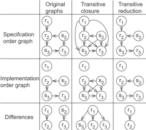
The unenforceable orders are identified by differentiating be-tween the specification order graph and the implementation order graph. Essentially, both graphs represent partially ordered sets with transitiveness. Thus, to obtain valid differences between them, the transitive closures of both graphs should be used in the differentiation. For example, in the first column of the table inFig. 12, the differences between the specification order graph and the implementation order graph in the original graph are the orders ‘‘r1tor2’’ and ‘‘s2tor3’’. However, the order ‘‘s2tor3’’ is tran-sitively satisfied in the implementation order graph. To avoid this, the transitive closures of both graphs should be used. However, a s₃ r₃ r₄ s₄ s₅ r₅ s₆ r₆ r₇ s₇ s₈ r₈ r₁ s₂ s₁ r₂

Fig. 10.Implementation order graph ofFig. 6.

sd SenderSendsData

Sensor Database Control pressure

sd TurnSensorOff Database Control Sensor 1 1 2 2

Fig. 11.Example for the non-local choice. EU

nl¼ ð

v

1;

v

2Þjlocð

v

1Þ–locð

v

2Þ;

v

1;

v

22 S;bsdð

v

1Þð

v

2Þ

v

1¼minðgU_djl1Þ;

v

2¼minðg U djl2Þ;g U d ¼suffixðU;dÞl1–l2;8l1;l22L;8d2 D n o suffixðU;dÞ ¼ S b1...bk2dbk...bn2PðIÞjB grefðbkÞ_{. . .}grefðbnÞ s₃ r₂ r₁ Specifcation order graph Implementation order graph Transitive reduction Transitive closure r₃ s₂ s₃ r₂ r₁ r₃ s₂ s₃ r₂ r₁ r₃ s₂ s₃ r₂ r₁ r₃ s₂ s₃ r₂ r₁ r₃ s₂ s₃ r₂ r₁ r₃ s₂ Differences s₃ r₂ r₁ r₃ r₂ r₁ Original graphs r₂ r₁ r₃ s₂

Fig. 12.Transitive closure and reduction.

1 _{The ‘‘Sensor’’ and ‘‘Control’’ have controls and there are neither communications}

nor coordinators between them. Note that a sending event can be controlled by a lifeline which has the sending event.

(8)

problem still remains. As shown in the second column of the table inFig. 12, the orders ‘‘r1tos3’’, ‘‘r1tor2’’ and ‘‘r1tor3’’ are the dif-ferences between the transitive closures of the two graphs. Only the order ‘‘r1tor2’’ is an essential cause because the absence of the order ‘‘r1tor2’’, which is originally given by the speciﬁcation, leads to the absence of the orders ‘‘r1tos3’’ and ‘‘r1tor3’’ as a result of the transitive closure. To minimize the result, we adopted the transitive reduction. It produces a minimal graph that preserves the same partial orderedness in the original one. With the transi-tive reduction, we can obtain the ﬁnal result as shown in the third column of the table inFig. 12.

However, the transitive reduction causes another problem although, in Fig. 12, the differentiation between the transitive reductions of the specification order graph and implementation or-der graph correctly identifies the unenforceable oror-ders. When the transitive reduction removes an order from a graph and does not remove the order from another graph, the order is identified as one of the unenforceable orders. Since the orders that are removed by the transitive reduction are always conserved by remaining or-ders, the causes that correspond to such orders are invalid. Thus, we calculate the differences between the transitive closure and transitive reduction of graphs in order to obtain the unenforceable orders.

Definition 12. The unenforceable orders for UML scenario speci-ficationUare defined as follows:

gU

cause¼gUnspec[gUnimpl

gU

nimpl¼trðgUspecÞ n ðgUimplÞ

gU

nspec¼trðgUimplÞ n ðgUspecÞ

wheretris a transitive reduction and⁄

is a transitive closure. The set minusg1ng2between the graphsg1= (E,V) andg2= (E0

,V) is deﬁned as (EnE0,V).

Due to the semantics of the set minusn, the unenforceable or-ders have two components:gU

nimplandgUnspec. Interestingly, the two components have different semantics:gU

nimplrepresents orders that are enforced in the scenario speciﬁcation, but that cannot be en-forced in the implementation model, andgU

nspec represents orders that should not be enforced, but that are held in the implementa-tion model. Therefore, when we interpret the unenforceable or-ders, such a difference should be considered.

Now, we describe the unenforceable orders detected in the example shown inFig. 6.Fig. 13shows the transitive reductions of the speciﬁcation and implementation order graphs shown in

Figs. 8 and 10. Since the example is small, inFig. 13, we can easily ﬁgure out differences between them; the bold solid lines represent gU

nspecand the bold dashed lines are gUnimpl. Overlapping the unen-forceable orders with the given scenario speciﬁcation helps to eas-ily understand them. Fig. 14 shows such an overlapped view. According to the semantics of gU

nspec andgUnimpl, we can interpret Fig. 14as follows: (1) ‘‘Delivery Dpt.’’ may receive a message ‘‘ deliv-eryOrder’’ before the message ‘‘product’’ arrives even though the sce-nario specification enforces that the message ‘‘deliveryOrder’’ is received after receiving the message ‘‘product’’. (2) Although the execution flow branches out of the ‘‘sddeliveryA’’ scenario, ‘‘Delivery Dpt.’’ may send the ‘‘deliveryB’’ message. (3) Although the execution flow branches out of the ‘‘sd deliveryB’’ scenario, ‘‘Delivery Dpt.’’ may send the ‘‘deliveryA’’ message.

5.2. Algorithms

In this section, we provide algorithms for detecting unenforce-able orders and analyze their complexity. Through the complexity, we want to show that our approach can be applied in the large-scale scenario specification and is more efficient than detecting the implied scenarios. According to the definition of the unenforce-able orders, we first describe algorithms for creating a specification

s₃ r₃ r₄ s₄ s 5 r 5 s₆ r₆ r₇ s₇ s 8 r 8 r 1 s₂ s 1 r₂ s₃ r₃ r₄ s₄ s 5 r 5 s₆ r₆ r₇ s₇ s 8 r 8 r 1 s₂ s 1 r₂

(a) Transitive reduction of specification order graph

(b) Transitive reduction of implementation order graph

: gnimpl : gnspec

Fig. 13.Transitive reductions ofFigs. 8 and 10.

sd deliveryA

requestA deliveryA deliveryOrder 3 3 4 5 5 4

sd deliveryB

requestB deliveryB deliveryOrder 6 6 7 8 8 7

sd produce Delivery Dpt. produce 1 1 Factory product 2 2

: NImpl

: NSpec

(9)

order graph and an implementation order graph. Then, the proce-dure for differentiating those two graphs will be shown.

Procedure 1shows an algorithm for creating a specification or-der graph. The procedure firstly removes control nodes from a bIOD: line 2. Then, it creates a specification order graph for each bSD: lines 5–16. At last, those specified properties of bSDs are asynchronously concatenated: lines 17–21. In the procedure, there are four undefined procedures: ‘‘removeControlNodes’’, ‘‘remove-Tau’’, ‘‘mins’’, and ‘‘ maxs’’. ‘‘removeControlNodes’’ and

‘‘remove-Tau’’ procedures remove control nodes of a bIOD and

s

from a speciﬁcation order graph, respectively. By modifying the transitive closure algorithm[17], we can easily implement them with worst-case complexityOðjVIj3Þand O(jVspecj3), respectively. The ‘‘mins’’

and ‘‘maxs’’ procedures return the ﬁrst and last vertices of a given

causal order graph if there is a vertex, respectively. Otherwise, they return

s. Note that, without the

s, the asynchronous concatenation

operator cannot be run, correctly. For example, if bSDsA,B, andC should be concatenated, and if theBdoes not have an event for life-linel, a last event onlinAis not concatenated with a ﬁrst event onl inCwithout

s.

Procedure 1. [createSpeciﬁcationOrderGraph]

Require:U: UML scenario speciﬁcation 1: ðB;I;refÞ U 2: ðEI;VIÞ removeControlNodes(I) 3: Espec ; 4: Vspec ; 5: for all

v

2VIdo 6: (Ob,Mb,Lb,locb, <b) ref(

v

) 7: for alll2Lbdo 8: for all(b,e)2<bjldo 9: Espec Espec[{(b,e)} 10: end for 11: end for 12: for all(s,r)2Mbdo 13: Espec Espec[{(s,r)} 14: end for 15: Vspec Vspec[Ob 16: end for 17: for allð

v

1;

v

2Þ 2EIs.t.

ref(

v

1) = (O1,M1,L1,loc1, <1),ref(

v

2) = (O2,M2,L2,loc2, <2)do 18: for alll2L1[L2do

19: Espec Espec[{(maxs(<1jl),mins(<2jl))} 20: end for

21: end for

22: return(removeTau(Espec),Vspec)

With appropriate data structures, the complexity ofProcedure 1

is bound toOðjVIjjLbjj<bjlj þ jEIjjL1[L2j þ jVIj3þ jVspecj3Þ: the ﬁrst and second terms correspond to the ﬁrstfor all(lines 5–16) and secondfor all(lines 17–21), respectively, and the third and fourth terms correspond to ‘‘removeControlNodes’’ and ‘‘removeTau’’, respectively. Roughly, the complexity ofProcedure 1is abstracted toO(jVspecj3).

Procedure 2. [prepareHistory]

Require: (Espec,Vspec): Speciﬁcation order graph

1: h empty history function

2: for all

v

2Vspecdo 3: h(

v

) (;,lbl(

v

))

4: end for

5: for alll2Ltotaldo 6: for all(

v

1,

v

2)2Especdo

7: if

v

1and

v

2is onl, and

v

2is receiving eventthen

8: (H,lb) h(

v

2) 9: h(

v

2) (H[{h(

v

1)},lb) 10: end if 11: end for 12: end for 13: returnh

Procedure 2returns a history function, which returns states of each vertex of the speciﬁcation order graph. This procedure is needed to obtain the permutating orders.

It begins by setting a history function of each vertex to an empty set: lines 2–4. Then, for each lifeline l and each edge (

v

1,

v

2), if a vertex

v

1 is a predecessor of

v

2 on the same life-line l, then

v

1’s history is added to the history of

v

2: lines 5– 12.

The complexity ofProcedure 2 is roughly bound toO(jVspecj2) becausejLtotalj6jVspecjandjEspecj6jVspecj.

Procedure 3. [ﬁrstReactEvent]

Require:

v

: a vertex of a bIOD,l: a lifeline,V: a set of visited vertices

1: r empty set

2: if

v

RVthen

3: V V[{

v

}

4: if

v

is not a control node andref(

v

) has an event on the lifelinelthen

5: (Ob,Mb,Lb,locb, <b) ref(

v

) 6: ifmin(<bjl) is a sending eventthen 7: r r[{min(<bjl)}

8: end if

9: else

10: for allv0₂_{a set of next nodes of}

_v

_do 11: r r[ﬁrstReactEvent(

v

0_,_l₎

12: end for

13: end if

14: end if

15: returnr

Procedure 3is a helper procedure for detecting non-local choice orders. It returns a ﬁrst event for the given lifeline after the given vertex, and is bound toO(jVIj+jEIj) since it is a kind of a Depth First Search (DFS) algorithm.

Procedure 4. [detectNonLocalChoiceOrder]

Require:U: UML scenario speciﬁcation,Eimpl: Set of edges of implementation order graph

1: ðB;I;refÞ U 2: ðEI;VIÞ I

3: Ltotal union of all lifelines inB 4: DI a set of decision vertices inVI 5: for all

v

2DIdo

6: S empty set

7: for alll2Ltotaldo

8: Sl empty set

9: N_v a set of next nodes of

v

10: for allv0₂_N vdo

(10)

12: Sl Sl[e 13: for alls2Sdo 14: Eimpl Eimpl[{(s,e)} 15: Eimpl Eimpl[{(e,s)} 16: end for 17: end for 18: S S[Sl 19: end for 20: end for 21: returnEimpl

Procedure 4is a procedure for creating the non-local choice or-ders. For each decision node and each lifeline, it ﬁnds a ﬁrst send-ing event throughProcedure 3. Then, edges between every pair of the events is added to the implementation order graph, except in the case in which a pair of events is on the same lifeline or in the same bSD.

The complexity ofProcedure 4is bound toOðjDIjjLtotaljjNvjðjSjþ jEIj þ jVIjÞÞ, andO(jVspecj3) can be roughly used as a concise form of the complexity.2

Procedure 5. [createImplementationOrderGraph]

Require:U: UML scenario speciﬁcation, (Espec,Vspec):speciﬁcation order graph 1: Eimpl ;

2: for all(

v

1,

v

2)2Especdo

3: if

v

2is a sending event or (

v

1,

v

2) is originated from a messagethen

4: Eimpl Eimpl[{(

v

1,

v

2)}

5: end if

6: end for

7: h prepareHistory(gspec) 8: for all

v

12Vspecdo 9: for all

v

22Vspecdo

10: ifh(

v

1) =h(

v

2) and

v

1–

v

2then 11: for all

v

32Vspecand (

v

2,

v

3)2Especdo 12: if

v

3and

v

2is on the same lifelinethen 13: Eimpl Eimpl[{(

v

1,

v

3)} 14: end if 15: end for 16: end if 17: end for 18: end for

19: Eimpl detectNonLocalChoiceOrder(U;Eimpl)

20: Eimpl

Procedure 5presents an algorithm for creating the implementa-tion order graph. First, in lines 2–6, the uncertain orders are re-moved from the speciﬁcation order graph. Before adding the permutating orders, the procedure prepares the history function usingProcedure 2. Then, in lines 8–18, the permutating orders are added to the implementation order graph: for every pair of dis-tinct events

v

1and

v

2, if they have the same history, edges between them their very next events are inserted. Note that we do not need to returnVimpllikeProcedure 1becauseVimplis the same withVspec. The complexity ofProcedure 5is clearlyO(jVspecj3).

Procedure 6. [detectUnenforceableOrders]

Require:U:UML 2.0 scenario speciﬁcation

1: (Espec,Vspec) createSpeciﬁcationOrderGraph(U) 2: Eimpl createImplementationOrderGraph((Espec,Vspec))

3: Eþ

spec transitiveClosure(Espec)

4: Eþ

impl transitiveClosure(Eimpl)

5: E spec transitiveReduction(E spec) 6: Eimpl transitiveReduction(E impl)

7: Enspec ;,Vnspec ;,Enimpl ;,Vnimpl ; 8: for allðe;e0Þ 2E

impldo 9: ifðe;e0ÞRE specthen 10: Enspec Enspec[{(e,e0)} 11: Vnspec Vnspec[{e,e0} 12: end if 13: end for

14: for allðe;e0Þ 2E

specdo 15: ifðe;e0ÞRE implthen 16: Enimpl Enimpl[{(e,e0)} 17: Vnimpl Vnimpl[{e,e0} 18: end if 19: end for

20: (Enspec,Vnspec), (Enimpl,Vnimpl)

Finally, our main algorithm is described inProcedure 6. First of all, the speciﬁcation order graph and implementation order graph are created byProcedures 1 and 5. Then, their transitive closures and transitive reductions are calculated. Finally, their differences are calculated in lines 8–19.

The complexity ofProcedures 1 and 5is roughlyO(jVspecj3), and the transitive closure and transitive reduction also haveO(jVspecj3) complexity using Warshall’s algorithm[17]. Therefore, the com-plexity of our whole approach is bound toO(jVspecj3). This complex-ity is relatively acceptable for the large-scale scenario speciﬁcation because it is polynomial.

Now, let’s compare our approach with the prior approaches that detect the implied scenarios. As we mentioned previously, such works synthesize an automata-based model, which is created by parallel compositions between local automata that represent life-lines’ behaviors. According to[1], under the asynchronous commu-nication style, the realizability check for scenarios with loops is undecidable if sizes of queues, that used to store received messages between agents, are not bound. Even though the queue sizes are bound, the state space of such approaches is still exponential to the size of queues under the asynchronous communication style[1]. The synchronous communication is a special case that the size of queue is zero: the number of states of the synthesized automa-ton is given asjQ1j. . .jQnjwhereQ1,. . .,Qnare states of local auto-mata. In worst case, the events are equally distributed to each local automaton:Qi=jVspecj/nandi= 1. . .nwhereVspecis a set of events. Therefore, the space complexity of the synthesized autom-aton isOððjVspecj

n Þ

n

Þ. Whennis 2, previous approaches show better performance than ours, while, when n is larger than 3, our ap-proach shows better performance than others.

Therefore, we can argue that, in case of large scenarios, our ap-proach is generally more efﬁcient than prior apap-proaches that de-tect the implied scenarios, especially under the asynchronous communication style.

6. Supporting other communication styles

In Section5, we explained the detection of unenforceable orders under the asynchronous communication style.

2

jSj þ jEIj þ jVIj6_a_jVspecjandjDIjjNvjjLtotalj6_jEIjjLtotalj6_jVIj2jLtotalj6_jVIjjVspecj6 jVspecj2.

(11)

The asynchronous communication style enforces only the or-ders between the sending event and their corresponding receiving event for messages, which are already included in the specification order graph and implementation order graph. However, in other communication styles, more orders are enforced. Hence, to support the other communication styles, the specification order graph and implementation order graph should have additional orders to re-flect their characteristics. In this subsection, we describe such addi-tional orders for supporting the following communication styles.

FIFO communication.A message sender does not wait for the arrival of the message at the receiver. A message sent ﬁrst is received ﬁrst.

Synchronous communication. A message sender waits until the message arrives at the receiver.

In the FIFO communication style, messages are received in the order in which the messages are sent. InFig. 15, the message ‘‘ ques-tionnaire’’ is sent from the object ‘‘Producer’’ to the object ‘‘Consumer’’ before the message ‘‘advertise’’. Under the FIFO communication style, the message ‘‘questionnaire’’ always arrives before the mes-sage ‘‘advertise’’. Thus, the order between the receiving events of the messages ‘‘questionnaire’’ and ‘‘advertise’’ is conserved, although the order is the uncertain order. To reﬂect such conservation, the implementation order graph should have additional orders be-tween the receiving events, in a lifeline, corresponding to the send-ing events that have orders between them. We refer to such orders as theFIFO orders. The FIFO orders are already included in the spec-iﬁcation order graph. Thus, under the FIFO communication style, they are only added to the implementation order graph. Their def-inition is as follows:

Deﬁnition 13. Let x and y be receiving events such that loc(x) =loc(y), and (x,y)2E for a speciﬁcation order graph gU

spec¼ ðE;VÞ. Likewise, letx0andy0be sending events of messages

whose receiving events arexandy, respectively. Ifloc(x0_{) =}_loc₍_y0_), then the order ‘‘xtoy’’ is the FIFO order.

Figs. 16 and 17present the speciﬁcation order graph, imple-mentation order graph, and unenforceable orders for the bSD shown in Fig. 15 under asynchronous communication style and FIFO communication style, respectively. According to the above

deﬁnition, inFig. 17, the order ‘‘r1tor3’’ is the FIFO order. There-fore, inFig. 17b, the order ‘‘r1tor3’’ is included in the implemen-tation order graph. Under asynchronous communication style, the order ‘‘r1 tor3’’ is an unenforceable order. However, under FIFO communication style, it does not cause implied scenarios due to the FIFO orders as shown inFig. 17c.

Now, we explain the additional orders for synchronous commu-nication. In synchronous communication, after an object sends a message, the object waits until the message is received by another object. This means that no event can occur in the object before the receiving event of the message. Thus, for each message, the speci-ﬁcation order graph and implementation order graph should have an order enforcing that the receiving event occur before any subse-quent events. Those orders are referred to assynchronous orders. They are formally deﬁned as follows:

Deﬁnition 14. Letxandybe the sending event and receiving event of a message, respectively. Also, letz be the very next sending event of x in the lifeline of x. Then, the order ‘‘y to z’’ is the synchronous order.

Fig. 18shows the speciﬁcation order graph and implementation order graph under the synchronous communication style. In

Fig. 15, after sending the message ‘‘questionnaire’’, the object ‘‘ Pro-ducer’’ waits until the receiving event r1 arises. In other words, the events2always arises after the eventr1. To reﬂect such charac-teristics, the speciﬁcation order graph and implementation order graph should have the order ‘‘r1tos2’’, the synchronous order. Sim-ilarly, the order ‘‘r2tos3’’ should also be added. Due to the synchro-nous orders, the bSD, shown in Fig. 15, does not have any unenforceable orders under synchronous communication style.

7. Case study

In this section, we present two case studies for scenario speciﬁ-cations on a boiler control system and mobility management in a Global Systems for Mobile communications (GSM) network. The purpose of the former case study is to show the usefulness of identifying the unenforceable orders in dealing with the implied

Producer Store questionnaire advertise put

s

₁

r

₁

s

₂

r

₃

s

₃

r

₂ Consumer get

r

₄

s

₄ Fig. 15.Example bSD. r₁ s₂ s₁ r₂ r₃ s₃ s₄ r₄ r₁ s₂ s₁ r₂ r₃ s₃ s₄ r₄

(a) Specified order graph (b) Implementation order graph r₁ r₂ r₃ r₄ (c) Causes of implied scenarios Fig. 16.Graphs generated from the bSD inFig. 15under asynchronous commu-nication style. r₁ s₂ s₁ r₂ r₃ s₃ s₄ r₄ r₁ s₂ s₁ r₂ r₃ s₃ s₄ r₄

(a) Specified order graph (b) Implementation order graph r₂ r₄ (c) Causes of implied scenarios : FIFO orders

Fig. 17.Graphs generated from the bSD inFig. 15under FIFO communication style.

r₁ s₂ s₁ r₂ r₃ s₃ s₄ r₄ r₁ s₂ s₁ r₂ r₃ s₃ s₄ r₄

(a) Specified order graph

(b) Implementation order graph

: synchronous orders

Fig. 18.Graphs generated from the bSD inFig. 15under synchronous communi-cation style.

(12)

scenarios, and to show that our approach provides more ﬁne-grained detection than recent approaches. Through the latter case study, we show the importance in considering various communica-tion styles and the performance of our algorithm. These case studies were carried out on a computer with the following speciﬁ-cations: Intel(R) Quad Core 3 Ghz, 4GB with Windows 7 64bit. Our tool is implemented as an Eclipse plug-in and it uses the Eclipse UML plug-in. There are pure Java and Java Native Interface (JNI) versions, but, in these case studies, we use only the pure Java ver-sion. The implementation and results of the case studies can be downloaded fromhttp://se.kaist.ac.kr/.

7.1. Boiler control system

We borrowed a scenario specification of a boiler control system from[9,15]. The scenario specification in[9,15]is described with the MSC. We converted it into a form of UML scenario specification. This example originally consists of four MSCs and an hMSC with 14 events. The application of our loop unrolling produces 12 MSCs and an hMSC, with 34 events in them. The seven unenforceable orders are detected under the synchronous communication style, as shown inFig. 19.

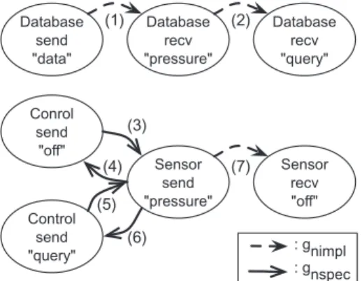
InFig. 19, the detected unenforceable orders are shown as lines: the dashed lines denotegnimplthat represents orders which are en-forced in the scenario specification but cannot be enen-forced in the implementation model, while the solid lines denotegnspecthat rep-resents orders which should not be enforced, but are held in the implementation model. The parenthesized number beside each unenforceable order is its identifier. Each circle represents an event whose label consists of the name of a lifeline holding the event, the type of event, and the name of a message related to the message, from the first line.

To get an intuitive viewpoint, we overlay those unenforceable orders on the scenario speciﬁcation[15,9], as shown in Fig. 20. According to the semantics ofgnimplandgnspec, each of the unen-forceable orders inFig. 20is interpreted as follows:

Unenforceable order.(1) The scenario speciﬁcation enforces that the ‘‘Database’’ receives the message ‘‘pressure’’ after sending of the message ‘‘data’’. However, the message ‘‘pressure’’ may arrive before the sending. The ‘‘Sensor’’ does not know about the inter-nal state of the ‘‘Database’’, so the ‘‘Sensor’’ may send the mes-sage ‘‘pressure’’ before sending the message ‘‘data’’.

Unenforceable order.(2) The scenario speciﬁcation enforces that the ‘‘Database’’ receives the message ‘‘query’’ after receiving the message ‘‘pressure’’. However, the message ‘‘query’’ may arrive before the reception of the message ‘‘pressure’’. The ‘‘Sensor’’ and ‘‘Control’’ do not know about each other’s internal state,

so the ‘‘Control’’ may send the message ‘‘query’’ before ‘‘Sensor’’ sends the message ‘‘pressure’’.

Unenforceable orders.(3), (4) The scenario speciﬁcation enforces that the sending events for the message ‘‘off’’ and ‘‘pressure’’ should not occur concurrently. However, after the decision node ‘‘d’’, those events may simultaneously occur.3_{At the}

deci-sion node ‘‘d’’, the ‘‘Sensor’’ and ‘‘Control’’ independently make a decision, so that the ‘‘Sensor’’ may proceed to ‘‘sdSensorSendsData’’, while the ‘‘Control’’ may proceed to ‘‘sdTurnSensorOff’’. Then, they may make send the messages ‘‘pressure’’ and ‘‘off’’ concurrently. Unenforceable orders.(5), (6) The scenario speciﬁcation enforces that the sending events for the message ‘‘query’’ and ‘‘pressure’’ should not occur concurrently. However, after the decision node ‘‘d’’, those events may simultaneously occur.3

At the decision node ‘‘d’’, the ‘‘Sensor’’ and ‘‘Control’’ indepen-dently make a decision, so that the ‘‘Sensor’’ may proceed to ‘‘sd SensorSendsData’’ while the ‘‘Control’’ may proceed to ‘‘sd

CommandActuator’’. Then they may send the messages ‘‘pressure’’ and ‘‘query’’ concurrently.

Unenforceable order.(7) The scenario speciﬁcation enforces that the ‘‘Sensor’’ receives the message ‘‘off’’ after sending the mes-sage ‘‘pressure’’. However, the message ‘‘off’’ may arrive before sending the message ‘‘pressure’’. The ‘‘Control’’ does not know about the internal state of the ‘‘Sensor’’, so the ‘‘Control’’ may send the message ‘‘off’’ before sending the message ‘‘pressure’’.

For the comparative case study, we choose Letier et al.’s work

[9]since only the work covered the input–output implied scenar-ios among the related works. However, there were no its concrete and full implementations. Thus, we manually made LTSs according to their approach and used Labeled Transition System Analyzer (LTSA)[14] for calculating the implied scenarios. The LTSs used for this case study can be downloaded inhttp://se.kaist.ac.kr/.

Fig. 21shows the detected implied scenarios and corresponding unenforceable orders which are detected by our approach. All de-tected implied scenarios correspond to a subset of the unenforce-able orders. Therefore, we can argue that our approach is consistent with previous approaches.

As shown inFig. 21, the implied scenario is just an error trace. Such error traces do not identify which part of the scenario speci-fication leads to the implied scenarios. Thus, using existing ap-proaches, the designer who wants to treat the implied scenarios should compare the implied scenarios with the scenario specifica-tion. On the other hand, in our approach, the unenforceable orders reveal where the problems exist and what events are relevant to the problems, as shown inFig. 20. For example, through the unen-forceable order (2) inFig. 21, a designer can focus on devising a means to coordinate the receiving events of the message ‘‘pressure’’ and ‘‘query’’ without analysis of the implied scenario. Therefore, we argue that identifying the causes of implied scenarios provides an easier means for treating the implied scenarios than just providing the implied scenarios, particularly in the large scenario specification.

Interestingly, the unenforceable orders (1) and (5) inFig. 21are related to one implied scenario. In this case, both of them should be coordinated in order to remove the implied scenario. Therefore, without the unenforceable orders, handling the implied scenarios may become harder.

Fig. 22shows the implied scenarios that are not detected by Letier et al.’s work, but that are detected by our approach.4_They Database send "data" Database recv "pressure" Database recv "query" Sensor send "pressure" Sensor recv "off" Conrol send "off" Control send "query" (1) (2) (3) (4) (5) (6) (7) : g_nimpl : g_nspec

Fig. 19.Unenforceable orders in the boiler control system under synchronous communication style.

3

Note that each pair of the unenforceable orders ‘‘(3) and (4)’’ and ‘‘(5) and (6)’’ make a cycle. This means that events in the cycle may occur simultaneously.

4_{In fact, our approach only detect the unenforceable orders. However, we can drive}

the implied scenarios from the speciﬁcation order graph and the unenforceable orders.

(13)

assume the synchrony hypothesis between the sending and receiv-ing events of a message, while we do not. Through the difference, our approach can detect more implied scenarios.

It is worth noting that some of the detected implied scenarios in

Fig. 22do not seem to be the implied scenarios(second and third ones). For example, if the boiler control system proceed along se-quences of bSDs ‘‘sd TurnSensorOn’’, ‘‘sd SensorSendsData’’, ‘‘sd

SensorSendsData’’, and ‘‘sdTurnSensorOff’’, the second implied sce-nario is explicitly presented in the scesce-nario speciﬁcation. However, the detected unenforceable order (4) explains another case. On the decision node ‘‘d’’, the ‘‘Sensor’’ can choose the path to the bSD ‘‘sd

SensorSendsData’’, while the ‘‘Control’’ can take a path to the bSD ‘‘sd

TurnSensorOff’’. Then, the bSD ‘‘sd TurnSensorOff’’ and ‘‘sd Sensor-SendsData’’ are concurrently executed. The ﬁrst and second implied scenarios inFig. 22represent this phenomenon, and they are def-initely undesired scenarios.

7.2. Mobility management in a GSM network

We borrowed a scenario speciﬁcation describing mobility man-agement in a GSM network from[10]. The speciﬁcation consists of

14 MSCs and an hMSC that combines the MSCs. It has 128 events and four lifelines. After the loop unrolling, we obtained 84 MSCs and an hMSC with 420 events. Since this speciﬁcation has ﬁve loops, and because four loops of them are nested, many duplica-tions of MSCs occur.

This scenario speciﬁcation has 55 unenforceable orders with the asynchronous communication style. Under the FIFO communica-tion style and synchronous communicacommunica-tion style, 42 and 32 unen-forceable orders are detected, respectively. These results let us know that the communication style signiﬁcantly affects the im-plied scenarios. Thus, to guarantee the absence of the imim-plied sce-narios, the appropriate communication style should be considered.

Fig. 23shows one of the unenforceable orders detected from the scenario speciﬁcation under the asynchronous and FIFO communi-cation style. The bold line denotes a detected unenforceable order. It describes that the receiving event of the message ‘‘ CON-NECT_ACK’’ can arise after the receiving event of the message ‘‘DISC’’. In the synchronous communication style, the object ‘‘MS’’ waits until the message ‘‘CONNECT_ACK’’ arrives at the object ‘‘MSC’’. After the arrival, the messages ‘‘DISCON’’ and ‘‘DISC’’ can be sent. Therefore, under the synchronous communication style, Sensor Database Control

on

off

Actuator Sensor Database Control

on

query

Actuator

Sensor Database Control

on

query

pressure

Actuator

pressure

Detected implied scenarios

Corresponding unenforced orders

Database recv "pressure" Database recv "query" (2) Sensor send "pressure" Sensor recv "off" (7) Database send "data" Database recv "pressure" (1) Sensor send "pressure" Control send "query" (5)

Fig. 21.Implied scenarios detected by previous approaches[9], and corresponding unenforceable orders.

sd CommandActuator

sd TurnSensorOn

Sensor Database Control Actuator

on

sd SensorSendsData

pressure

Sensor Database Control Actuator

query

sd TurnSensorOff

off data command : gnimpl : gnspec (1) (2) (3) (4) (5) (6) (7) d