arXiv:1407.4504v2 [cs.DC] 2 Sep 2014
1
Hybrid Random/Deterministic Parallel Algorithms
for Nonconvex Big Data Optimization
Amir Daneshmand, Francisco Facchinei, Vyacheslav Kungurtsev, and Gesualdo Scutari
(the order of the authors is alphabetical
∗)
Abstract—We propose a decomposition framework for the
parallel optimization of the sum of a differentiable (possibly nonconvex) function and a nonsmooth (possibly nonseparable), convex one. The latter term is usually employed to enforce structure in the solution, typically sparsity. The main contribution of this work is a novel parallel, hybrid random/deterministic de-composition scheme wherein, at each iteration, a subset of (block) variables is updated at the same time by minimizing local convex approximations of the original nonconvex function. To tackle with huge-scale problems, the (block) variables to be updated are chosen according to a mixed random and deterministic procedure, which captures the advantages of both pure deterministic and random update-based schemes. Almost sure convergence of the proposed scheme is established. Numerical results show that on huge-scale problems the proposed hybrid random/deterministic algorithm outperforms both random and deterministic schemes.
Index Terms—Nonconvex problems, Parallel and distributed
methods, Random selections, Jacobi method, Sparse solution.
I. INTRODUCTION
We consider the minimization of the sum of a smooth (possibly nonconvex) functionF and of a nonsmooth (possibly nonseparable) convex one G:
min
x∈XV(x),F(x) +G(x), (1)
where X is a closed convex set with a cartesian product structure:X= ΠN
i=1Xi⊆Rn. Our focus is on problems with
a huge number of variables, as those that can be encountered, for example, in machine learning, compressed sensing, data mining, tensor factorization and completion, network opti-mization, image processing, genomics, and meteorology. We refer the reader to [1]–[13] and the books [14], [15] as entry points to the literature.
Recent years have witnessed a surge of interest in these very large scale problems, and the evocative term Big Data opti-mization has been coined to denote this new area of research. Block Coordinate Descent (BCD) methods rapidly emerged as a winning paradigm to attack Big Data optimization, see e.g. [3]. At each iteration of a BCD method one block of variables is updated using first-order information, while keeping all other variables fixed. This dramatically reduces the memory and computational requirements of each iteration and leads to simple and scalable methods. One of the key ingredients in a BCD method is the choice of the block of variables
∗All the authors contributed equally to the paper.
A. Daneshmand and G. Scutari are with the Dept. of Electrical Engi-neering, at the State Univ. of New York at Buffalo, Buffalo, USA. Email: <amirdane,gesualdo>@buffalo.edu.
F. Facchinei is with the Dept. of Computer, Control, and Manage-ment Engneering, at Univ. of Rome La Sapienza, Rome, Italy. Email: [email protected].
V. Kungurtsev is with the Agent Technology Center, Dept. of Computer Science, Faculty of Electrical Engineering, Czech Technical University in Prague. Email:[email protected].
Part of this work has been published on arxiv on June 2014.
to update. This can be accomplished in several ways, for example using a cyclic order or some greedy/opportunistic selection strategy, which aims at selecting the block leading to the largest decrease of the objective function. The cyclic order has the advantage of being extremely simple, but the greedy strategy usually provides faster convergence, at the cost of an increased computational effort at each iteration. However, no matter which block selection rule is adopted, as the dimensions of the optimization problems increase, even BCD methods may result inadequate. To alleviate the “curse of dimensionality”, three different kind of strategies have been proposed, namely: (a) parallelism, where several blocks of variables are updated simultaneously in a multicore or distributed computing environment, see e.g. [5]–[7], [7]–[10], [16]–[25]; (b) random selection of the block(s) of variables to update, see e.g. [20]–[30]; and (c) use of “more-than-first-order” information, for example (approximated) Hessians or (parts of) the original function itself, see e.g. [4], [18], [19], [31], [32]. Point (a) is self-explanatory and rather intuitive (although the corresponding theoretical analysis is by no means trivial); here we only remark that the vast majority of parallel BCD methods apply to convex problems only. Points (b) and (c) need further comments.
Point (b): The random selection of variables to update (also termed random sketching) is essentially as cheap as a cyclic selection while alleviating some of the pitfalls of cyclic rules. Moreover, random sketching is relevant in distributed environments wherein data are not available in their entirety, but are acquired either in batches over time or over a network (and not all nodes are equally responsive). In such scenarios, one might be interested in running the optimization process at a certain instant even with the limited, randomly available information. The main limitation of random selection rules is that they remain disconnected from the status of the optimiza-tion process, which instead is exactly the kind of behavior that greedy-based updates try to avoid, in favor of faster convergence, but at the cost of more intensive computation.
Point (c): The use of “more-than-first-order” information also has to do with the trade-off between cost-per-iteration and overall cost of the optimization process. Using higher order or structural information may seem unreasonable, given the huge size of the problems at hand, and in fact the accepted wisdom is that at most first-order information can be used in the Big Data environment. However, recent studies, as those mentioned above, challenge this wisdom and suggest that a judicious use of some kind of “more-than-first-order” information can lead to substantial overall improvements.
The above pros& cons analysis suggests that it would be desirable to design a parallel algorithm for nonconvex prob-lems combining the benefits of random sketching and greedy updates, possibly using “more-than-first-order” information.
To the best of our knowledge, no such algorithm exists in the literature. In this paper, building on our previous deterministic methods [18], [19], [33], we propose a BCD-like scheme for the computation of stationary solutions of Problem (1) filling the gap and enjoying all the following features:
1) It uses a random selection rule for the blocks, followed by a deterministic subselection;
2) It can classically tackle separable convex functionG, i.e., G(x) =PiGi(xi), but also nonseparable functionsG; 3) It can deal with a nonconvex functionsF;
4) It can use both first-order and higher-order information; 5) It is parallel;
6) It can use inexact updates;
7) It converges almost surely, i.e. our convergence results are of the form “with probability one”.
As far as we are aware of, this is the first algorithm enjoying all these properties, even in the convex case. The combination of all the features 1-7 in one single algorithm is a major achievement in itself, which offers great flexibility to develop tailored instances of solutions methods within the same frame-work (and thus all converging under the same unified condi-tions). Last but not least, our experiments show impressive performance of the proposed methods, outperforming state-of-the-art solution scheme (cf. Sec. IV). As a final remark, we underline that, at more methodological level, the combination of all features 1-7 and, in particular, the need to conciliate random and deterministic strategies, led to the development of a new type of convergence analysis (see Appendix A) which is also of interest per se and could bring to further developments. Below we further comment on some of features 1-7, com-pare to existing results, and detail our contributions.
Feature 1: As far as we are aware of, the idea of making a random selection and then perform a greedy subselection has been previously discussed only in [34]. However, re-sults therein i) are only for convex problems with a specific structure; ii) are based on a regularized first-order model; iii) require a very stringent “spectral-radius-type” condition, which severely limits the degree of parallelism−the maximum number of variables that can be simultaneously updated at each iteration while guaranteeing convergence; and iv) convergence results are in terms of expected value of the objective function. The proposed algorithmic framework expands vastly on this setting, while enjoying also all properties 2-7. In particular, it is the first hybrid random/greedy scheme for nonconvex nonseparable functions, and it allows any degree of parallelism (i.e., the update of any number of variables); and all this is achieved under much weaker convergence conditions than those in [34], satisfied by most of practical problems. Numer-ical results show that the proposed hybrid schemes updating greedily just some blocks within the pool of those selected by a random rule is very effective, and seems to preserve the advantages of both random and deterministic selection rules.
Feature 2: The ability of dealing with some classes of nonseparable convex functions has been documented in [35]– [37], but only for deterministic and sequential schemes; our approach extends also to parallel, random schemes.
Feature 3: The list of works dealing with BCD methods for nonconvex F’s is short: [22], [29] for random sequential
methods; and [7], [17]–[19], [38] for deterministic parallel ones. The only (very recent) paper dealing with random parallel methods for nonconvexF’s is the arxiv submission [38], which however does not enjoy the key properties 1, 2, and 6.
Feature 4: We want to stress the ability of the proposed algorithm to exploit in a systematic way “more-than-first-order” information. At each iteration of a BCD method, one block of variables is updated using a (possibly regularized) first-order model of the objective function, while keeping all other variables fixed. Our method, following the approach first explored in [18], [19], [33] provides the flexibility of using more sophisticated models. For example, i) one could use a Newton-like approximation; or ii) suppose that in (1) F =
F1+F2, whereF1is convex andF2is not. Then, at iterationk,
one could base the update of thei-th block on the approximant F1(xi,xk−i)+∇xiF2(x
k)T(x
i−xki)+G(xi,xk−i), wherex−i
denotes the vector obtained from xby deletingxi. The logic
here is that instead of linearizing the whole functionFwe only linearize the difficult, nonconvex partF2. In this light we can
also better appreciate the importance of feature 6, since if we go for more complex approximants, the ability to deal with inexact solutions becomes important.
Feature 6: Inexact solution methods have been little stud-ied. Papers [3], [39], [40] (somewhat indirectly) consider some of these issues in the specialized context of ℓ2-loss linear
support vector machines. A more systematic treatment of in-exactness of the solution of a first-order model is documented in [41], in the context of random sequential BCD methods for convex problems. Our results in this paper are based on our previous works [18], [19], [33], where both the use of “more-than-first-order” models and inexactness are introduced and rigorously analyzed in the context of parallel, deterministic methods. This paper extends results in [18], [19], [33] to the random, parallel schemes for nonconvex objective functions, and constitute the first study of these issues in this setting.
As a final remark, we observe that a large portion of works mentioned so far are interested in (global) complexity analysis. Of course this is an important topic, but it is outside the scope of this paper. Note that, with the exception of [29], all papers dealing with complexity analyses, study (regularized) gradient-type methods for convex problems. Given our ex-panded setting, we believe it is more fruitful to concentrate on proving convergence and verifying the practical effectiveness of our algorithms.
The paper is organized as follows. Section II formally introduces the optimization problem along with the main assumptions under which it is studied and also discusses some technical points. The proposed algorithmic framework and its convergence properties are introduced in Section III, while numerical results are presented in Section IV. Section V draws some conclusions. All proofs are given in the Appendix.
II. PROBLEMDEFINITION ANDPRELIMINARIES We consider Problem (1), where the feasible set X =
X1× · · · ×XN is a Cartesian product of lower dimensional
convex setsXi⊆Rni, andx∈Rn is partitioned accordingly:
3
N , {1, . . . , N} the set of the N blocks. The function F is smooth (and not necessarily convex and separable) and G is convex, and possibly nondifferentiable and non-separable. Some widely-used choices for G(x) are ckxk1
and cPNi=1kxik2, from which one can see that Problem
(1) includes many popular Big Data optimization problems, such as Lasso, group Lasso, sparse logistic regression, ℓ2
-loss Support Vector Machine, Nuclear Norm Minimization, and Nonnegative Matrix (or Tensor) Factorization problems.
Assumptions. Given (1), we make the following blanket
assumptions:
(A1) EachXi is nonempty, closed, and convex;
(A2) F isC1 on an open set containingX;
(A3) ∇F is Lipschitz continuous onX with constantLF;
(A4) G is continuous and convex onX (possibly nondiffer-entiable and nonseparable);
(A5) V is coercive.
Note that the above assumptions are standard and are satisfied by most of the problems of practical interest. For instance, A3 holds automatically if X is bounded, whereas A5 guarantees the existence of a solution.
With the advances of multi-core architectures, it is desirable to develop parallel solution methods for Problem (1) whereby operations can be carried out on some or (possibly) all (block) variables xi at the same time. The most natural parallel
(Jacobi-type) method one can think of is updating all blocks simultaneously: given xk, each (block) variablex
i is updated
by solving the following subproblem
xki+1∈argmin
xi∈Xi
F(xi,xk−i) +G(xi,xk−i) . (2) Unfortunately this method converges only under very restric-tive conditions [42] that are seldom verified in practice (even in the absence of the nonsmooth partG). Furthermore, the exact computation ofxki+1 may be difficult and computationally too expensive.
To cope with these issues, a natural approach is to replace the (nonconvex) functionF(•, xk
−i)by a suitably chosen local
convex approximationFei(xi;xk), and solve instead the convex problems (one for each block)
xki+1∈argmin xi∈Xi n ˜ hi(xi;xk),Fei(xi;xk) +G(xi;xk−i)o, (3) with the understanding that the minimization in (3) is simpler than that in (2). Note that the functionGhas not been touched; this is because i) it is generally much more difficult to find a “good” approximation of a nondifferentiable function than of a differentiable one; ii) G is already convex; and iii) the functions G encountered in practice do not make the optimization problem (3) difficult (a closed form solution is available for a large classes ofG’s, ifFei(xi;xk)are properly
chosen). In this work we assume that the approximation functions Fei(z;w) : Xi ×X → R, have the following
properties (we denote by ∇Fei the partial gradient of Fei with
respect to the first argumentz):
(F1) Fei(•;w)is uniformly strongly convex with constantq >
0 onXi;
(F2) ∇Fei(xi;x) =∇xiF(x)for allx∈X;
(F3) ∇Fei(z;•)is Lipschitz continuous onX for allz∈Xi.
Such a functionFeishould be regarded as a (simple) convex
approximation ofF at the pointx with respect to the block of variables xi that preserves the first order properties of F
with respect toxi. Note that, contrary to most of the works in
the literature (e.g., [37]), we do not requireFei to be a global
upper approximation of F, which significantly enlarges the range of applicability of the proposed solution methods.
The most popular choice forFei satisfying F1-F3 is e Fi(xi;xk) =F(xk) +∇xiF(x k)T(x i−xki) + τi 2kxi−x k ik 2, (4) with τi > 0. This is essentially the way a new iteration is
computed in most (block-)BCDs for the solution of (group) LASSO problems and its generalizations. When G ≡ 0, this choice gives rise to a gradient-type scheme; in fact we obtainxki+1 simply by a shift along the antigradient. As we discussed in the introduction, this is a first-order method, so it seems advisable, at least in some situations, to use more informativeFei-s. IfF(xi,xk−i)is convex, an alternative
is to take Fei(xi;xk) as a second order approximation of
F(xi,xk −i), i.e., e Fi(xi;xk) =F(xk) +∇ xiF(x k)T(x i−xki) +12(xi−xki)T ∇2xixiF(x k) +qI(x i−xki), (5) where q is nonnegative and can be taken to be zero if F(xi,xk−i) is actually strongly convex. When G ≡ 0, this
essentially corresponds to taking a Newton step in minimizing the “reduced” problemminxi∈XiF(xi,x
k
−i). Still in the case
of convexF(xi,xk−i), one could also take just e
Fi(xi;xk) =F(xi,xk−i),
which preserves the whole structure of the function. Other valuable choices tailored to specific applications are discussed in [19], [33]. As a guideline, note that our method, as we shall describe in details shortly, is based on the iterative (approximate) solution of problem (3) and therefore a balance should be aimed at between the accuracy of the approximation
˜
F and the ease of solution of (3). Needless to say, the option (4) is the less informative one, although it usually makes the computation of the solution of (3) a cheap task.
Best-response map: Associated with each i and point xk ∈
X, under F1-F3, we can define the following optimal block solution map: b xi(xk),argmin xi∈Xi ˜ hi(xi;xk). (6)
Note thatbxi(xk)is always well-defined, since the optimization
problem in (6) is strongly convex. Given (6), we can then introduce the solution map
X ∋y7→bx(y),(bxi(y))Ni=1. (7) Our algorithmic framework is based on solving in parallel a suitable selection of subproblems (6), converging thus to fixed-points ofbx(•)(of course the selection varies at each iteration). It is then natural to ask which relation exists between these
fixed points and the stationary solutions of Problem (1). To answer this key question, we recall first a few definitions.
Stationarity: A point x∗ is a stationary point of (1) if a subgradient ξ ∈ ∂G(x∗) exists such that (∇F(x∗) +ξ)T(y−x∗)≥0 for ally∈X.
Coordinate-wise stationarity: A point x∗ is a coordinate-wise stationary point of (1) if subgradients ξi ∈ ∂ξiG(x
∗), with i ∈ N, exist such that (∇x
iF(x∗) +
ξi)T(y
i−x∗i)≥0, for all yi∈Xi andi∈ N.
Of course, if F is convex, stationary points coincide with its global minimizers. In words, a coordinate-wise stationary solution is a point for whichx∗is stationary w.r.t. every block of variables. It is clear that a stationary point is always a coordinate-wise stationary point; the converse however is not always true, unless extra conditions onGare satisfied.
Regularity: Problem (1) is regular at a coordinate-wise
sta-tionary point x∗ if x∗ is also a stationary point of the problem.
Regularity at x∗ is a rather weak requirement, and is easily seen to be implied, in particular, by the following two conditions:
(a) Gis separable (still nonsmooth), i.e.,G(x) =PiGi(xi);
(b) Gis continuously differentiable aroundx∗.
Note that (a) is assumed in practically all papers dealing with deterministic/random BCD methods (with the exception of [36], [37], where however only sequential schemes are proposed). Regularity can well occur also for nonseparable functions. For instance, consider the function arising in logistic regression problems F(x) = Pmj=1log(1 +e−aij
yT
jx), with
X = Rn, and y
j ∈ Rn and aj ∈ {−1,1} being given
constants. Now, chooseG(x) =ckxk2; the resulting function
is continuously differentiable, and therefore regular, at any stationary point but x∗ 6= 0. It is easy to verify that V is also regular at x=0, provided thatc <log 2.
The following proposition is elementary and elucidates the connections between stationarity conditions of Problem (1) and fixed-points ofxb(•).
Proposition 1. Given Problem (1) under A1-A5 and F1-F3,
the following hold:
i) The set of fixed-points of xb(•) coincides with the coordinate-wise stationary points of Problem (1);
ii) If, in addition, Problem (1) is regular at a fixed-point of
b
x(•), then such a fixed-point is also a stationary point of the problem.
Other properties of the best-response map bx(•) that are instrumental to prove convergence of the proposed algorithm are introduced in Appendix B.
III. ALGORITHMICFRAMEWORK
We are ready to describe our algorithmic framework. We begin introducing a formal description of its salient character-istic, the novel hybrid random/greedy block selection rule.
The random block selection works as follows: at each iteration k, a random set Sk ⊆ N is generated, and the
blocks i∈ Sk are the potential candidate variables to update
in parallel. The set Sk is a realization of a random set-valued
mappingSk with values in the power set ofN. To keep the proposed scheme as general as possible, we do not constraint
Sk to any specific distribution; we only require that, at each iteration k, each block i has a chance (positive probability, possibly nonuniform) to be selected.
(A6) The setsSk are realizations of independent random
set-valued mappings Sk such that P(i ∈ Sk) ≥ p, for all
i= 1, . . . , N andk∈N+, and some p >0.
A random selection rule Sk satisfying A6 will be called proper sampling. Several proper sampling rules will be dis-cussed in details shortly.
As already discussed in the introduction, the random se-lection of blocks seems becoming beneficial when the di-mensions of the problem increase significantly. But recent results in [10], [19], [43], [44] strongly suggest that a greedy approach updating only the “promising” blocks is an impor-tant ingredient of an efficient algorithm. Of course, for very large scale problems, checking whether a block is promising or not might become computationally demanding and thus time consuming. To avoid this burden while capturing the benefits of both strategies, the proposed approach consists in combining random and greedy updates in the following form. First, a random selection is performed−the set Sk is
generated. Second, a greedy procedure is run to select in the poolSkonly the subset of blocks, saySˆk, that are “promising”
(according to a prescribed criterion). Finally all the blocks in
ˆ
Skare updated in parallel. To complete the description of such
an hybrid random/greedy selection, the notion of “promising” block needs to be made formal, which is done next.
Since xk
i is an optimal solution of (6) if and only if b
xi(xk) = xk
i, a natural distance of xki from the optimality
is dk
i , kbxi(xk)−xkik. The blocks in Sk to be updated
can be then chosen based on such an optimality measure (e.g., opting for blocks exhibiting larger dk
i ’s). However,
this choice requires the computation of the solutions bxi(xk),
for all i ∈ Sk, which in some applications might be still
computationally too expensive. Building on the same idea, we can introduce alternative, less expensive metrics by replacing the distance kbxi(xk)−xkik with a computationally cheaper error bound, i.e., a functionEi(x) such that
sikxbi(xk)−xkik ≤Ei(xk)≤¯sikxbi(xk)−xkik, (8)
for some0<si≤¯si. Of course one can always setEi(xk) =
kbxi(xk)−xkik, but other choices are also possible, we refer the interested reader to [19] for more details.
The proposed hybrid random/greedy scheme capturing all the features 1)-6) discussed in Sec. I is formally given in Algorithm 1. Note that in step S.3 inexact calculations of bxi
are allowed, which is another noticeable and useful feature: one can reduce the cost per iteration without affecting too much, experience shows, the empirical convergence speed. In step S.5 we introduced a memory in the variable updates: the new point xk+1 is a convex combination via γk of xk and b
zk. The step-sizeγk plays a key rule in the convergence, and
needs to be properly tuned, as specified in Theorem 2, which summarizes the convergence properties of Algorithm 1.
5
Algorithm 1: Hybrid Random/Deterministic Flexible Par-allel Algorithm (HyFLEXA)
Data:{εk
i}fori∈ N,τ ≥0,{γk}>0,x0∈X,ρ∈(0,1].
Setk= 0.
(S.1): Ifxk satisfies a termination criterion: STOP;
(S.2):Randomly generate a set of blocksSk⊆ {1, . . . , N}
(S.3): SetMk ,max
i∈Sk{Ei(xk)}.
Choose a subset Sˆk⊆ Sk that contains at least one indexi for whichEi(xk)≥ρMk.
(S.4): For alli∈Sˆk, solve (6) with accuracyεk i : findzk i ∈Xi s.t. kzki −bxi xk k ≤εk i;
Setbzki =zki fori∈Sˆk andbzk
i =xki fori6∈Sˆk (S.5): Setxk+1,xk+γk(bzk
−xk);
(S.6): k←k+ 1, and go to (S.1).
Theorem 2. Let {xk} be the sequence generated by
Algo-rithm 1, under A1-A6. Suppose that {γk} and {εk
i} satisfy
the following conditions: i) γk ∈ (0,1]; ii) γk → 0;
iii) Pkγk = + ∞; iv) Pk γk2 < + ∞; and v) εk i ≤ γkα 1min{α2,1/k∇xiF(x
k)k} for all i ∈ N and some
nonnegative constants α1 and α2. Additionally, if inexact
solutions are used in Step 3, i.e., εk
i > 0 for some i and
infinite k, then assume also that G is globally Lipschitz on X. Then, either Algorithm 1 converges in a finite number of iterations to a fixed-point ofˆx(•)of (1) or there exists at least one limit point of {xk}that is a fixed-point of ˆx(•)w.p.1.
Proof: See Appendix C.
The convergence results in Theorem 2 can be strengthened when Gis separable.
Theorem 3. In the setting of Theorem 2, suppose in addition
that G(x) is separable, i.e., G(x) = Pi∈NGi(xi). Then, either Algorithm 1 converges in a finite number of iterations to a stationary solution of Problem (1) or every limit point of
{xk} is a stationary solution of Problem (1) w.p.1.
Proof: See Appendix D.
On the random choice of Sk. We discuss next some proper
sampling rulesSk that can be used in Step 3 of the algorithm
to generate the random sets Sk; for notational simplicity the iteration index k will be omitted. The sampling rule S is
uniquely characterized by the probability mass function P(S),P(S=S), S ⊆ N,
which assign probabilities to the subsetsS ofN. Associated with S, define the probabilities qj , P(|S| = j), for
j = 1, . . . , N. The following proper sampling rules, proposed in [25] for convex problems with separable G, are instances of rules satisfying A6, and are used in our computational experiments.
− Uniform (U) sampling. All blocks get selected with the same (non zero) probability:
P(i∈S) =P(j∈S) = E[|S|]
N , ∀i6=j∈ N.
−Doubly Uniform (DU) sampling. All setsS of equal cardi-nality are generated with equal probability, i.e.,P(S) =P(S′), for all S,S′
⊆ N such that |S|=|S′
|. The density function
is then
P(S) = q|S| n
|S|
.
− Nonoverlapping Uniform (NU) sampling. It is a uniform sampling rule assigning positive probabilities only to sets forming a partition ofN. LetS1, . . . ,SP be a partition ofN,
with eachSi>0, the density function of the NU sampling is: P(S) = 1 P, ifS ∈ S1, . . . , SP 0 otherwise
which corresponds toP(i∈ S) =N/P, for all i∈ N. A special case of the DU sampling that we found very effective in our experiments is the so called “nice sampling”.
−Nice Sampling (NS). Given an integer0≤τ ≤N, aτ-nice sampling is a DU sampling with qτ = 1 (i.e., each subset of
τ blocks is chosen with the same probability).
The NS allows us to control the degree of parallelism of the algorithm by tuning the cardinalityτ of the random sets generated at each iteration, which makes this rule particularly appealing in a multi-core environment. Indeed, one can set τ equal to the number of available cores/processors, and assign each block coming out from the greedy selection (if implemented) to a dedicated processor/core.
As a final remark, note that the DU/NU rules contain as special cases fully parallel and sequential updates, wherein at each iteration a single block is updated uniformly at random, or all blocks are updated.
−Sequential sampling: It is a DU sampling with q1 = 1, or
a NU sampling withP =N andSj=j, forj= 1, . . . , P.
−Fully parallel sampling: It is a DU sampling withqN = 1,
or a NU sampling withP = 1andS1=N.
Other interesting uniform and nonuniform practical rules (still satisfying A6) can be found in [25], [45], to which we refer the interested reader for further details..
On the choice of the step-sizeγk. An example of step-size
rule satisfying Theorem 2i)-iv) is: given0< γ0≤1, let
γk=γk−1 1−θ γk−1, k= 1, . . . , (9) where θ ∈ (0,1) is a given constant. Numerical results in Section IV show the effectiveness of (9) on specific prob-lems. We remark that it is possible to prove convergence of Algorithm 1 also using other step-size rules, including a standard Armijo-like line-search procedure or a (suitably small) constant step-size. Note that differently from most of the schemes in the literature, the tuning of the step-size does not require the knowledge of the problem parameters (e.g., the Lipschitz constants of∇F andG).
IV. NUMERICALRESULTS
In this section we present some preliminary experiments providing a solid evidence of the viability of our approach; they clearly show that our framework leads to practical meth-ods that exploit well parallelism and compare favorably to existing schemes, both deterministic and random.
Because of space limitation, we present results only for (synthetic) LASSO problems, one of the most studied in-stances of (the convex version of) Problem (1), corresponding
to F(x) = kAx−bk2, G(x) = ckxk1, and X = Rn.
Extensive experiments on more varied (nonconvex) classes of Problem (1) are the subject of a separate work.
All codes have been written in C++ and use the Message Passing Interface for parallel operations. All algebra is per-formed by using the Intel Math Kernel Library (MKL). The algorithms were tested on the General Compute Cluster of the Center for Computational Research at the SUNY Buffalo. In particular for our experiments we used a partition composed of 372 DELL 32x2.13GHz Intel E7-4830 Xeon Processor nodes with 512 GB of DDR4 main memory and QDR InfiniBand 40Gb/s network card.
Tuning of Algorithm 1: The most successful class of random
and deterministic methods for LASSO problem are (proximal) gradient-like schemes, based on a linearization of F. As a major departure from current schemes, here we propose to better exploit the structure of F and use in Algorithm 1 the following best-response: given a scalar partition of the variables (i.e., ni= 1for alli), let
b xi(xk),argmin xi∈R n F(xi,xk−i) + τi 2(xi−x k i)2+λ|xi| o . (10) Note that bxi(xk)has a closed form expression (using a
soft-thresholding operator [8]).
The free parameters of Algorithm 1 are chosen as follows. The proximal gainsτiand the step-sizeγare tuned as in [19,
Sec. VI.A]. The error bound function is chosen as Ei(xk) =
kbxi(xk)−xikk, and, for any realizationSk, the subsetsSˆk in S.3 of the algorithm are chosen as
ˆ
Sk=
{i∈ Sk :Ei(xk)
≥σMk
}. (11)
We denote by cSk the cardinality of Sk normalized to the
overall number of variables (in our experiments, all sets Sk have the same cardinality, i.e., cSk = cS, for all k). We
considered the following options for σ and cS: i) cS = 0.01,0.1,0.2,0.5,0.8; ii)σ= 0, which leads to a fully parallel pure random scheme wherein at each iteration all variables in
ˆ
Sk are updated; and iii) different positive values ofσranging
from 0.01to0.5, which corresponds to updating in a greedy manner only a subset of the variables inSˆk (the smaller theσ
the larger the number of potential variables to be updated at each iteration). We termed Algorithm 1 withσ= 0 “Random FLEXible parallel Algorithm” (RFLEXA), whereas the other instances with σ >0 as “Hybrid FLEXA” (HyFLEXA).
Algorithms in the literature: We compared our versions of
(Hy)FLEXA with the most representative parallel random and deterministic algorithms proposed in the literature to solve the convex instance of Problem (1) (and thus also LASSO). More specifically, we consider the following schemes.
• PCDM & PCDM2: These are (proximal) gradient-like
parallel randomized BCD methods proposed in [25] for convex optimization problems. Since the authors recommend to use PCDM instead of PCDM2 for LASSO problems, we do so (indeed, our experiments show that PCDM outperforms PCDM2). We simulated PCDM under different sampling rules and we set the parametersβ andωas in [25, Table 4], which guarantees convergence of the algorithm in expected value.
• Hydra& Hydra2: Hydra is a parallel and distributed ran-dom gradient-like CDM, proposed in [46], wherein different cores in parallel update a randomly chosen subset of variables from those they own; a closed form solution of the scalar updates is available. Hydra2[20] is the accelerated version of Hydra; indeed, in all our experiments, it outperformed Hydra; therefore, we will report the results only for Hydra2. The free parameterβ is set to β = 2β∗
1 (cf. Eq. (15) in [46]), with σ
given by Eq. (12) in [46] (according to the authors, this seems one of the best choices forβ).
• FLEXA: This is the parallel deterministic scheme we
proposed in [18], [19]. We use FLEXA as a benchmark of deterministic algorithms, since it has been shown in [18], [19] that it outperforms current (parallel) first-order (accelerated) gradient-like schemes, including FISTA [8], SparRSA [9], GRock [10], parallel BCD [7], and parallel ADMM. The free parameters of FLEXA, τi and γ, are tuned as in [19, Sec.
VI.A], whereas the set Sk is chosen as in (11).
•Other algorithms: We tested also other random algorithms,
including sequential random BCD-like methods and Shotgun [16]. However, since they were not competitive, to not over-crowd the figures, we do not report results for these algorithms. In all the experiments, the data matrixA= [A1· · · AP]of
the LASSO problem is stored in a column-block manner, uni-formly across theP parallel processes. Thus the computation of each productAx (required to evaluate∇F) and the norm
kxk1(that isG) is divided into the parallel jobs of computing
Aixi andkxik1, followed by a reduce operation. Also, for all
the algorithms, the initial point was set to the zero vector.
Numerical Tests: We generated synthetic LASSO problems
using the random generation technique proposed by Nesterov [6], which we properly modified following [25] to generate instances of the problem with different levels of sparsity of the solution as well as density of the data matrixA∈Rm×n; we introduce the following two control parameters:sA=average
%of nonzeros in each column ofA(out ofm); andssol= %
of nonzeros in the solution (out ofn). We tested the algorithms on two groups of LASSO problems,A∈R104×105 andA∈
R105×106, and several degrees of density of A and sparsity of the solution, namelyssol = 0.1%,1%,5%,15%,30%, and
sA= 10%,30%,50%,70%,90%. Because of the space
limi-tation, we report next only the most representative results; we refer to [47] for more details and experiments. Results for the LASSO instance with 100,000 variables are reported in Fig. 1 and 2. Fig. 1 shows the behavior of HyFLEXA as a function of the design parameters σ and cS, for different values of the solution sparsity (ssol), whereas in Fig. 2 we compare
the proposed RFLEXA and HyFLEXA with FLEXA, PCDM, and Hydra2, for different values ofssol andsA(ranging from
“low” dense matrices and “high” sparse solutions to “high” dense matrices and “low” sparse solutions). Finally, in Fig. 3 we consider larger problems with 1M variables. In all the figures, we plot the relative errorre(x),(V(x)−V∗)/V∗ versus the CPU time, where V∗ is the optimal value of the objective functionV (in our experimentsV∗is known). All the curves are averaged over ten independent random realizations. Note that the CPU time includes communication times and the initial time needed by the methods to perform all pre-iterations
7
computations (this explains why the curves associated with Hydra2 start after the others; in fact Hydra2 requires some nontrivial computations to estimates β). Given Fig. 1-3, the following comments are in order.
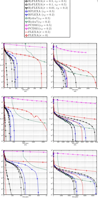
0 500 1000 1500 2000 2500 3000 3500 4000 10−6 10−5 10−4 10−3 10−2 10−1 100 time (sec) (a) re σ= 0.1,ssol= 0.2% σ= 0.5,ssol= 0.2% σ= 0.1,ssol= 2% σ= 0.5,ssol= 2% σ= 0.1,ssol= 5% σ= 0.5,ssol= 5% 0 500 1000 1500 2000 2500 3000 10−6 10−5 10−4 10−3 10−2 10−1 100 101 time (sec) (b) re cS= 0.5,ssol= 0.2% cS= 0.2,ssol= 0.2% cS= 0.1,ssol= 0.2% cS= 0.5,ssol= 2% cS= 0.2,ssol= 2% cS= 0.1,ssol= 2% cS= 0.5,ssol= 5% cS= 0.2,ssol= 5% cS= 0.1,ssol= 5%
Fig. 1: HyFLEXA for different values ofcS andσ: Relative error vs. time;
ssol= 0.2%,2%,5%,sA= 70%, 100.000 variables, NU sampling, 8 cores; (a)cS= 0.5, andσ= 0.1,0.5- (b)σ= 0.5, andcS= 0.1,0.2,0.5.
HyFLEXA: On the choice of(cS, σ), and the sampling strat-egy. All the experiments (including those that we cannot report here because of lack of space) show the following trend in the behavior of HyFLEXA as a function of (cS, σ). For “low” density problems (“low” ssol andsA), “large” pairs (cS, σ) are preferable, which corresponds to updating at each iteration only some variables by performing a (heavy) greedy search over a sizable amount of variables. This is in agreement with [19] (cf. Remark 5): by the greedy selection, Algorithm 1 is able to identify those variables that will be zero at the a solution; therefore updating only variables that we have “strong” reason to believe will not be zero at a solution is a better strategy than updating them all, especially if the solutions are very sparse. Note that this behavior can be obtained using either “large” or “small” (cS, σ). However, in the case of “low” dense problems, the former strategy outperforms the latter. We observed that this is mainly due to the fact that whensA is “small”, estimatingxˆi(computing
the products ATA) is computationally affordable, and thus performing a greedy search over more variables enhances the practical convergence. When the sparsity of the solution decreases and/or the density ofAincreases (“large”sAand/or
ssol), one can see from the figures that “smaller” values of (cS, σ)are more effective than larger ones, which corresponds to using a “less aggressive” greedy selection while searching over a smaller pool of variables. In fact, when A is dense, computing all xˆi might be prohibitive and thus nullify the
potential benefits of a greedy procedure. For instance, it follows from Fig. 1-3 that, as the density of the solution (ssol) increases the preferable choice for(cS, σ)progressively moves from (0.5,0.5) to (0.2,0.01), with both cS and σ decreasing. Interesting, a tuning that works quite well in practice for all the classes of problems we simulated (different densities of A, solution sparsity, number of cores, etc.) is
(cS, σ) = (0.5,0.1), which seems to strike a good balance between not updating variables that are probably zero at the optimum and nevertheless update a sizable amount of variables when needed in order to enhance convergence..
As a final remark, we report that, according to our
exper-0 5exper-0exper-0 re HyFLEXA(σ= 0.5,cS= 0.5) HyFLEXA(σ= 0.1,cS= 0.5) HyFLEXA(σ= 0.01,cS= 0.2) RFLEXA (cS= 0.5) RFLEXA (cS= 0.2) Hydra2(c S= 0.5) Hydra2(c S= 0.2) PCDM1(cS= 0.5) PCDM1(cS= 0.2) FLEXA(σ= 0.5) FLEXA(σ= 0) 0 50 100 150 200 250 300 350 10−6 10−5 10−4 10−3 10−2 10−1 100 101 102 time (sec) (a1) re 0 500 1000 1500 2000 2500 10−6 10−5 10−4 10−3 10−2 10−1 100 101 102 time (sec) (a2) re 0 500 1000 1500 2000 10−6 10−5 10−4 10−3 10−2 10−1 100 101 102 time (sec) (b1) re 0 500 1000 1500 2000 2500 3000 3500 4000 4500 10−6 10−5 10−4 10−3 10−2 10−1 100 101 102 time (sec) (b2) re 0 200 400 600 800 1000 10−6 10−5 10−4 10−3 10−2 10−1 100 101 102 time (sec) (c1) re 0 1000 2000 3000 4000 5000 10−6 10−5 10−4 10−3 10−2 10−1 100 101 102 time (sec) (c2) re
Fig. 2: LASSO with 100.000 variables, 8 cores; Relative error vs. time for: (a1)sA = 30%andssol = 0.2%- (a2)sA = 30%andssol = 5% -(b1)sA= 70%andssol= 0.2%- (b2)sA= 70%andssol= 5%- (c1) sA= 90%andssol= 0.2%- (c2)sA= 90%andssol= 5%.
iments, the most effective sampling rule among U, DU, NU, and NS is the NU (which is actually the one the figures refers to); NS becomes competitive only when the solutions are very sparse, see [47] for a detailed comparison of the different rules. Comparison of the algorithms. For low dense matrices A
and very sparse solutions, FLEXA σ = 0.5 is faster than its random counterparts (RFLEXA and HyFLEXA) as well as its fully parallel version, FLEXA σ = 0[see Fig 2 a1), b1) c1) and Fig. 3a)]. Nevertheless, HyFLEXA [with (cS, σ) = (0.5,0.5)]remains close. As already pointed out, this is mainly due to the fact that in these scenarios i) estimating all xˆi is
computationally cheap (and thus performing a greedy selection over a sizable set of variable is beneficial, see Fig. 1); and
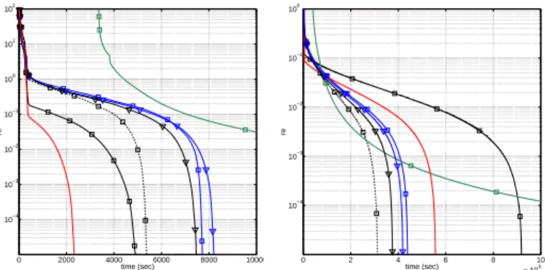
0 2000 4000 6000 8000 10000 10−4 10−3 10−2 10−1 100 101 102 time (sec) (a) re 0 2 4 6 8 10 x 104 10−4 10−3 10−2 10−1 100 time (sec) (b) re
Fig. 3: LASSO with 1M variables, sA= 10%, 16 cores; Relative error vs. time for: (a)ssol= 1%- (b)ssol= 5%. The legend is as in Fig. 2.
ii) updating only some variables at each iteration is more effective than updating all (FLEXA σ = 0.5 outperforms FLEXAσ= 0). However, as the density ofAand/or the size of the problem increase, computing all the products[ATA]ii
(required to estimate xˆi) becomes too costly; this is when a
random selection of the variables becomes beneficial: indeed, RFLEXA and HyFLEXA consistently outperform FLEXA [see Fig 2 a2), b2) c2) and Fig. 3b)]. Among the random algorithms, Hydra2 is capable to approach relatively fast low accuracy, especially when the solution is not too sparse, but has difficulties in reaching high accuracy. RFLEXA and HyFLEXA are always much faster than current state-of-the-art schemes (PCDM and Hydra2), especially if high accuracy of the solutions is required. Between RFLEXA and HyFLEXA (with the same cS), the latter consistently outperforms the former (about up to five time faster), with a gap that is more significant when solutions are sparse. This provides a solid evidence of the effectiveness of the proposed hybrid random/greedy selection method.
In conclusion, our experiments indicate that the proposed framework leads to very efficient and practical solution meth-ods for large and very large-scale (LASSO) problems, with the flexibility to adapt to many different problem characteristics.
V. CONCLUSIONS
We proposed a highly parallelizable hybrid random/deterministic decomposition algorithm for the minimization of the sum of a possibly noncovex differentiable function F and a possibily nonsmooth nonseparable convex function G. The proposed framework is the first scheme enjoying all the following features: i) it allows for pure greedy, pure random, or mixed random/greedy updates of the variables, all converging under the same unified set of convergence conditions; ii) it can tackle via parallel updates also nonseparable convex functions G; iii) it can deal with nonconvex nonseparable F; iv) it is parallel; v) it can incorporate both first-order or higher-order information; and vi) it can use inexact solutions. Our preliminary experiments on LASSO problems showed the superiority of the proposed scheme with respect to state-of-the-art random and deterministic algorithms. Experiments on more varied classes of problems are the subject of our current research.
VI. ACKNOWLEDGMENTS
The authors are very grateful to Prof. Peter Richtàrik for his invaluable comments; we also thank Dr. Martin Takáˇc and
Prof. Peter Richtàrik for providing the C++ code of PCDM and Hydra2(that we modified in order to use the MPI library).
The work of Daneshmand and Scutari was supported by the USA NSF Grants CMS 1218717 and CAREER Award No. 1254739. The work of Facchinei was supported by the MIUR project PLATINO (Grant Agreement n. PON01_01007). The work of Kungurtsev was supported by the European Social Fund under the Grant CZ.1.07/2.3.00/30.0034.
APPENDIX
We first introduce some preliminary results instrumental to prove both Theorem 2 and Theorem 3. Given Sˆk ⊆ N
and x , (xi)i∈N, for notational simplicity, we will denote by (x)k
ˆ
Sk (or interchangeably x k
ˆ
Sk) the vector whose
com-ponent i is equal to xi if i ∈ Sˆk, and zero otherwise.
With a slight abuse of notation we will also use (xi,y−i) to denote the ordered tuple(y1, . . . ,yi−1,xi,yi+1, . . . ,yN);
similarly (xi,xj,y−(i,j)), with i < j stands for
(y1, . . . ,yi−1,xi,yi+1, . . . ,yj−1,xj,yj+1, . . . ,yN).
A. On the random sampling and its properties
We introduce some properties associated with the random sampling rules Sk satisfying assumption A6. A key role in our proofs is played by the following random set: let{xk} be
the sequence generated by Algorithm 1, and ik
mx= argmax i∈{1,...,N}||b
xi(xk)−xki||, (12) define the setKmx as
Kmx, n
k∈N+ : ikmx∈Sko. (13) The key properties of this set are summarized in the following two lemmata.
Lemma 4 (Infinite cardinality). Given the setKmxas in (13),
it holds that
P(|Kmx|=∞) = 1, where|Kmx|denotes the cardinality of Kmx.
Proof: Suppose that the statement of the lemma is not true. Then, with positive probability, there must exist somek¯ such that fork≥¯k,ik
mx∈/ S
k. But we can write
P n ik mx∈/ Sk o k≥k¯ = Π k≥¯kP ik mx∈/S k |(i¯k mx∈/S ¯ k), . . . , (ik−1 mx ∈/S k−1) ≤ lim k→∞(1−p) k−¯k = 0.
where the inequality follows by A6 and the independence of the events. But this obviously gives a contradiction and concludes the proof.
Lemma 5. Let {γk
} be a sequence satisfying assumptions i)-iii) of Theorem 2. Then it holds that
P X k∈Kmx γk< ∞ ! = 0. (14) Proof:
9 It holds that, P X k∈Kmx γk< ∞ ! ≤ P [ n∈N X k∈Kmx γk< n ! ≤ X n∈N P X k∈Kmx γk< n ! . To prove the lemma, it is then sufficient to show that P P
k∈Kmxγ
k< n= 0, as proved next.
DefineKˆi, withi∈N+, as the smallest indexKˆi such that
ˆ Ki X j=0 γj ≥i·n. (15)
Note that sinceP∞k=0γk= +
∞,Kˆi is well-defined for alli
andlimi→∞Kˆi= +∞. For anyn∈N, it holds:
P X k∈Kmx γk< n ! =P \ m∈N m X k∈Kmx γk< n !! = lim m→∞P m X k∈Kmx γk< n ! = lim i→∞ P ˆ Ki X k∈Kmx γk< n = lim i→∞ P ˆ Ki X k∈Kmx γk < n, |Kmx∩[0,Kˆi]|< ˆ Ki √ i +P ˆ Ki X k∈Kmx γk< n, |Kmx∩[0,Kˆi]| ≥ ˆ Ki √ i ≤ lim i→∞ P |Kmx∩[0,Kˆi]|<K√ˆi i ! | {z } term I +P ˆ Ki X k∈Kmx γk< n, |Kmx∩[0,Kˆi]| ≥ ˆ Ki √ i | {z } term II . (16) Let us bound next “term I” and “term II” separately.
Term I: We have P |Kmx∩[0,Kˆi]|<K√ˆi i ! (a) = P ˆ Ki X k=0 Xk < ˆ Ki √ i ≤P ˆ Ki X k=0 Xk− ˆ Ki X k=0 pk > ˆ Ki X k=0 pk− ˆ Ki √ i (b) ≤ qP ˆ Ki k=0pk(1−pk) PKiˆ k=0pk− ˆ Ki √ i 2 (c) ≤ p ˆ Ki ˆ Ki p−√1 i 2 = p 1 ˆ Ki p−√1 i 2 −→ i→∞0 (17) where:
(a):X0, . . . ,XKiˆ are independent Bernoulli random variables,
with parameter pk , P(k ∈ Kmx). Note that, due to A6,
pk≥p, for allk;
(b): it follows from Chebyshev’s inequality;
(c): we used the bounds PKikˆ=0pk(1 − pk) ≤ Kˆi and PKiˆ
k=0pk ≥pKˆi.
Term II: Let us rewrite term II as P PKiˆ k∈Kmxγ k |Kmx∩[0,Kˆi]| < n |Kmx∩[0,Kˆi]| |Kmx∩[0,Kˆi]| ≥ ˆ Ki √ i ! ·P |Kmx∩[0,Kˆi]| ≥ K√ˆi i ! (a) ≤ P PKiˆ k∈Kmxγ k |Kmx∩[0,Kˆi]| < n √ i ˆ Ki |Kmx∩[0,Kˆi]| ≥ ˆ Ki √ i ! ·P |Kmx∩[0,Kˆi]| ≥ K√ˆi i ! (b) ≤ P PKiˆ k∈Kmxγ k |Kmx∩[0,Kˆi]| < PKiˆ k=0γk ˆ Ki √ i (c) ≤ P PKiˆ k=0γkXk ˆ Ki < PKiˆ k=0γk ˆ Ki 1 √ i ! ≤ P PKiˆ k=0γkXk ˆ K − PKiˆ k=0γkpk ˆ Ki > PKiˆ k=0γkpk ˆ Ki − PKiˆ k=0γk ˆ Ki 1 √ i ! ≤ P PKiˆ k=0γkXk ˆ Ki − PKiˆ k=0γkpk ˆ Ki > p−√1 i PKiˆ k=0γk ˆ Ki ! (d) ≤ qP ˆ Ki k=0(γk)2p(1−p) p−√1 i PKiˆ k=0γk 2 ≤ qP ˆ Ki k=0γk p−√1 i PKiˆ k=0γk 2 = 1 p−√1 i qPKiˆ k=0γk 2 −→ i→∞0, (18) where: (a): we used|Kmx∩[0,Kˆi]| ≥ ˆ Ki √
i, by the conditioning event;
(b): it follows from (15), andP(ATB)≤P(A);
(c):X0, . . . ,XKiˆ are independent Bernoulli random variables,
with parameterpk. The bound is due to|Kmx∩[0,Kˆi]| ≤Kˆi;
(d): it follows from the Chebyshev’s inequality.
The desired result (14) follows readily combining (16), (17), and (18).
B. On the best-response mapbx(•)and its properties We introduce now some key properties of the mappingxb(•)
defined in (6). We also derive some bounds involving xb(•)
along with the sequence{xk}generated by Algorithm 1.
Lemma 6 ([19]). Consider Problem (1) under A1-A5, and
with each Gi convex on Xi. Then the mapping X ∋ y 7→ b
x(y)is Lipschitz continuous onX, i.e., there exists a positive constantLˆ such that
kxb(y)−bx(z)k ≤ Lˆ ky−zk, ∀y,z∈X. (19)
Lemma 7. Let{xk}be the sequence generated by Algorithm 1. For every k ∈ Kmx and Sˆk generated as in step S.3
of Algorithm 1, the following holds: there exists a positive constantc1 such that,
||xˆSˆk(xk)−xSkˆk|| ≥c1||xˆ(x k)
−xk||. (20)
Proof: The following chain of inequalities holds:
max i∈N s¯i xˆSˆk(x k) −xkˆ Sk (≥a)¯sik ρ ˆxik ρ(x k) −xkik ρ (b) ≥Eik ρ(x k)(c) ≥ρ Eik mx(x k) (d) ≥ρ min i∈Nsi maxi∈N xˆi(xk)−xki ≥Nρ min i∈Nsi xˆ(x k) −xk where: in (a) ik
ρ is any index in Sˆk such that Eik ρ(x
k) ≥
ρmaxi∈SkEi(xk). Note that by definition ofSˆk (cf. step S.3
of Algorithm 1), such a index always exists; (b) is due to (8); (c) follows from the definition ofik
ρ, andmaxi∈SkEi(xk) =
Eik mx(x
k), the latter due to ik
mx ∈ Sk ⊇Sˆk (recall that k ∈
Kmx); and (d) follows from (8).
Lemma 8. Let{xk}be the sequence generated by Algorithm
1. For every k ∈ N+, and Sˆk generated as in step S.3, the
following holds: ∇xF(xk) T ˆ Sk bx(x k)−xk ˆ Sk ≤ −qk bx(x k)−xk ˆ Skk 2 +X i∈Sˆk G(xk)−G(xbi(xk),xk−i) . (21) Proof: Optimality ofxbi(xk)for the subproblemiimplies ∇xiFei(xbi(x k);xk) +ξ i(xbi(xk),xk−i) T yi−xbi(xk) ≥0, for all yi ∈ Xi, and some ξi(xbi(xk),xk−i) ∈
∂xiG(xbi(x k),xk −i). Therefore, 0≥ ∇xiFei(xbi(x k);xk)T bxi(xk)−xk i +ξi(xbi(xk),xk −i)T bxi(xk)−xki . (22)
Let us (lower) bound next the two terms on the RHS of (22). The uniform strong monotonicity ofFei(•;xk)(cf. F1),
∇xiFei(xbi(x k);xk) − ∇xiFei(x k i;xk) T (bxi(xk)−xki) ≥ q||bxi(xk)−xk i||2, (23) along with the gradient consistency condition (cf. F2)
∇xiFei(x k i;xk) =∇xiF(x k)imply ∇xiFei(bxi(x k);xk)T xbi(xk)−xk i =∇xiFei(bxi(x k);xk) − ∇xiFei(x k i;xk) T b xi(xk)−xki +∇xiFei(x k i;xk)T xbi(xk)−xki ≥ ∇xiF(x k)T bxi(xk)−xk i +q||bxi(xk)−xk i||2. (24) To bound the second term on the RHS of (22), let us invoke the convexity ofG(•,xk−i): G(xk i,xk−i)−G(xbi(xk),xk−i) ≥ξi(bxi(xk),xk −i)T xki −xbi(xk) , which yields ξi(xbi(xk),x−ki)T bxi(xk)−xki ≥G(bxi(xk),xk −i)−G(xk). (25)
The desired result (21) is readily obtained by combin-ing (22) with (24) and (25), and summcombin-ing overi∈Sˆk.
Lemma 9. Let{xk}be the sequence generated by Algorithm
1, and{γk} ↓0. For every k∈N
+ sufficiently large, andSˆk
generated as in step S.3, the following holds: G(xk+1)≤G(xk) +γkL GPi∈Sˆkεki +γk X i∈Sˆk G(bxi(xk),x−ki)−G(xk). (26) Proof: Givenk≥0 andSˆk, define¯xk,(¯xk
i)i∈N, with ¯ xki , xk i +γk bxi(xk)−xki , ifi∈Sˆk xk i otherwise.
By the convexity and Lipschitz continuity ofG, it follows G(xk+1) = G(xk) + G(xk+1) −G(¯xk) + G(¯xk)−G(xk) ≤ G(xk) +γkL G P i∈Sˆkεki + G(¯xk)−G(xk), (27)
where LG is a (global) Lipschitz constant of G. We bound
next the last term on the RHS of (27).
Let γ¯k = γkN, for k large enough so that 0 < γ¯k <1.
Definexˇk ,(ˇxk
i)i∈N, withˇxki =xki ifi /∈Sˆk, and ˇ
xki ,γ¯kxbi(xk) + (1−γ¯k)xki (28) otherwise. Using the definition of ¯xk it is not difficult to see
that ¯ xk= N−1 N x k+ 1 N xˇ k. (29)
Using (29) and invoking the convexity ofG, the following recursion holds for sufficiently largek:
G(¯xk) =G 1 N(ˇx k 1,xk−1) +N1(x k 1,ˇxk−1) +NN−2x k =G1 N (ˇxk1,xk−1) +NN−1 xk 1,N1−1ˇxk−1+NN−−21xk−1 ≤ N1 G xˇ k 1,xk−1 +N−1 N G x1k,N1−1xˇk−1+N−2 N−1x k −1 = N1 G xˇk1,xk−1+N−1 N G 1 N−1 xk1,xˇk−1 +N−2 N−1xk
11 =N1G xˇk 1,xk−1 +N−1 N G 1 N−1 ˇxk2,xk−2 +N1−1xk 1,xk2,ˇxk−(1,2) +N−3 N−1xk = 1 NG xˇk1,xk−1 +N−1 N G 1 N−1 ˇxk2,xk−2 +N−2 N−1 xk 1,xk2,N1−2xˇk−(1,2)+NN−−32xk−(1,2) ≤ 1 NG xˇ k 1,xk−1 +N1 G xˇk 2,xk−2 +N−2 N−1G xk 1,xk2,N1−2ˇxk−(1,2)+NN−−32xk−(1,2) ≤ ... ≤ N1 X i∈N G(ˇxki,xk−i). (30) Using (30), the last term on the RHS of (27) can be upper bounded for ksufficiently large as
G(¯xk)−G(xk)≤ N1 X i∈N G(ˇxki,xk−i)−G(xk) = 1 N X i∈Sˆk G(ˇxki,xk−i)−G(xk) (a) ≤ N1 X i∈Sˆk ¯ γkG(xbi(xk),xk−i) + (1−¯γk)G(xk)−G(xk) =γk X i∈Sˆk G(bxi(xk),x−ki)−G(xk), (31) where (a) is due to the convexity of G(•,xk
−i) and the
definition of ˇxk
i [cf. (28)].
The desired inequality (26) follows readily by combining (27) with (31).
Lemma 10. [48, Lemma 3.4, p.121] Let {Xk
}, {Yk
}, and
{Zk
}be three sequences of numbers such thatYk
≥0for all k. Suppose that Xk+1 ≤Xk−Yk+Zk, ∀k= 0,1, . . . and P∞k=0Zk < ∞. Then either Xk → −∞ or else {Xk }
converges to a finite value and P∞k=0Yk<∞.
C. Proof of Theorem 2
For any given k ≥ 0, the Descent Lemma [42] yields: with bzk , (bzk
i)i∈N and zk , (zki)i∈N defined in step S.4
of Algorithm 1, F xk+1 ≤ F xk+γk∇ xF xk T b zk−xk + γ k2L ∇F 2 bzk−xk2. (32)
We bound next the second and third terms on the RHS of (32). Denoting bySˆ
k
the complement ofSˆk, we have,
∇xF xk T bzk−xk =∇xF xk T b zk−xb(xk) +bx(xk)−xk (a) = ∇xF xk T ˆ Sk(zk−xb(xk))Sˆk +∇xF xk T ˆ Sk(x k−bx(xk)) ˆ Sk +∇xF xk T ˆ Sk(bx(xk)−xk)Sˆk +∇xF xk T ˆ Sk(bx(x k) −xk)ˆ Sk =∇xF xk T ˆ Sk(zk−xb(xk))Sˆk +∇xF xk T ˆ Sk(bx(x k) −xk)Sˆk (b) ≤ X i∈Sˆk εk i ∇xiF(x k) +∇xF xk T ˆ Sk(bx(x k) −xk)Sˆk (c) ≤ X i∈Sˆk εk i ∇xiF(x k) −qk bx(xk)−xkSˆkk 2 +X i∈Sˆk G(xk)−G(bxi(xk),xk−i) (33) where in (a) we used the definition ofbzk and of the setSˆk; in
(b) we usedzk
i −bxi(xk) ≤εk
i; and (c) follows from (21)
(cf. Lemma 8).
The third term on the RHS of (32) can be bounded as
bzk−xk2 ≤ 2 zk−xˆ(xk) ˆ Sk 2 +2 xˆ(xk)−xk ˆ Sk 2 = +2Pi∈Sˆk zk i −xbi(xk) 2 +2 xˆ(xk)−xkˆ Sk 2 ≤ 2 X i∈Sˆk (εki)2+ 2 xˆ(xk)−xkˆ Sk 2, (34) where the first inequality follows from the definition ofzk and b
zk, and in the last inequality we usedzk
i −bxi(xk) ≤εk
i.
Now, we combine the above results to get the descent property of V along {xk}. For sufficiently large k ∈ N
+, it holds V(xk+1) =F(xk+1) +G(xk+1) ≤V xk−γk q−γkL ∇F bx(xk)−xk ˆ Sk 2 +Tk, (35) where the inequality follows from (21), (32), (33), and (34), andTk is given by Tk,γk X i∈N εk i LG+ ∇xiF(x k)+ γk2L ∇F X i∈N (εk i) 2.
By assumption (iv) in Theorem 2, it is not difficult to show thatP∞k=0Tk<∞. Since γk →0, it follows from (35) that
k, say¯k, such that V(xk+1)≤V(xk)−γkβ 1 bx(xk)−xkˆ Sk 2+Tk, (36)
for allk≥¯k. Invoking Lemma 10 while usingP∞k=0Tk<
∞
and the coercivity of V, we deduce from (36) that
lim t→∞ t X k=¯k γk bx(xk)−xk ˆ Sk 2<+∞, (37) and thus also
lim t→∞ t X Kmx∋k≥¯k γk bx(xk)−xkˆ Sk 2 <+∞. (38) Lemma 5 together with (38) imply
lim inf k∈Kmx bx(xk)−xkˆ Sk = 0, w.p.1, which by Lemma 7 implies
lim inf k→∞
bx(xk)−xk= 0, w.p.1. (39) Therefore, the limit point of the infimum sequence is a fixed point ofbx(·)w.p.1.
D. Proof of Theorem 3
The proof follows similar ideas as the one of Theorem 1 in our recent work [19], but with the nontrivial complication of dealing with randomness in the block selection.
Given (39), we show next that, under the separability assumption on G, it holds that limk→∞
bx(xk)−xk = 0
w.p.1. For notational simplicity, let us define △bx(xk) , b
x(xk)−xk.
Note first that for any finite but arbitrary sequence{k, k+ 1, ..., ik−1}, it holds that E " ik−1 X Kmx∋t=k γt # = ikX−1 t=k γt[P(t∈ K mx)]≥p ikX−1 t=k γt, and thus P ikX−1 Kmx∋t=k γt> β ikX−1 t=k γt ! >0,
for all k∈ K and0< β < p. This implies that, w.p.1, there exists an infinite sequence of indexes, sayK1⊆ K, such that
ikX−1 Kmx∋t=k γt> β ikX−1 t=k γt, ∀k∈ K1. (40)
Suppose now, by contradiction, that
lim supk→∞
△xb(xk) > 0 with a positive probability. Then we can find a realization such that at the same time (40) holds for some K1 andlim supk→∞
△bx(xk)>0. In
the rest of the proof we focus on this realization and get a contradiction, thus proving that lim supk→∞
△bx(xk) = 0
w.p.1.
If lim supk→∞
△bx(xk) >0 then there exists a δ > 0
such that △bx(xk) > 2δ for infinitely many k and also
△bx(xk) < δ for infinitely many k. Therefore, one can always find an infinite set of indexes, say K, having the
following properties: for any k ∈ K, there exists an integer ik > ksuch that
△xb(xk)< δ, △bx(xik)>2δ (41) δ≤△xb(xj)≤2δ k < j < ik. (42)
Proceeding now as in the proof of Theorem 2 in [19], we have: fork∈ K1, δ (<a) △xb(xik)−△bx(xk) ≤ bx(xik)−bx(xk)+xik−xk (43) (b) ≤ (1 + ˆL)xik−xk (44) (c) ≤ (1 + ˆL) ikX−1 t=k γt △xb(xt)St +(zt−bx(xt))St (d) ≤ (1 + ˆL) (2δ+εmax) ikX−1 t=k γt, (45)
where (a) follows from (41); (b) is due to Lemma 6; (c) comes from the triangle inequality, the updating rule of the algorithm and the definition of bzk; and in (d) we used (41), (42), and
kzt−bx(xt)k ≤P
i∈Nεti, where εmax , maxk P
i∈Nεki <
∞. It follows from (45) that
lim inf K1∋k→∞ ikX−1 t=k γt ≥ δ (1 + ˆL)(2δ+εmax)>0. (46)
We show next that (46) is in contradiction with the con-vergence of {V(xk)}. To do that, we preliminary prove that,
for sufficiently large k ∈ K, it must be △xb(xk) ≥ δ/2.
Proceeding as in (45), we have: for any givenk∈ K,
△bx(xk+1)
−△xb(xk)≤(1 + ˆL)xk+1
−xk
≤(1 + ˆL)γk △bx(xk)+εmax.
It turns out that for sufficiently large k ∈ K1 so that (1 +
ˆ
L)γk < δ/(δ+ 2εmax), it must be
△xb(xk)≥δ/2; (47) otherwise the condition △xb(xk+1) ≥δ would be violated [cf. (42)]. Hereafter we assume without loss of generality that (47) holds for all k ∈ K1 (in fact, one can always restrict
{xk}k∈K1 to a proper subsequence).
We can show now that (46) is in contradiction with the convergence of {V(xk)}. Using (36) (possibly over a subse-quence), we have: for sufficiently largek∈ K1,
V(xik)≤V(xk)−β 1 ikX−1 Kmx∋t=k γt △bx(xt)Sˆt 2 + ikX−1 Kmx∋t=k Tt (a) ≤ V(xk)−β2 ikX−1 Kmx∋t=k γt△xb(xt)2+ ikX−1 t=k Tt (b) ≤V(xk)−β 3 ikX−1 t=k γt+ ikX−1 t=k Tt, (48) where (a) follows from Lemma 7 and β2 = c1β1 >0; and