Maximum likelihood drift estimation for a threshold diffusion

(1)

für Angewandte Analysis und Stochastik

Leibniz-Institut im Forschungsverbund Berlin e. V.

Preprint

ISSN 2198-5855

Maximum likelihood drift estimation for a threshold diffusion

Antoine Lejay

1,2

, Paolo Pigato

3 submitted: March 22, 2018 1 Université de Lorraine, CNRS IECL UMR 7502 54600 Vandœuvre-lès-Nancy France E-Mail: [email protected] 2 Inria 54600 Villers-lès-Nancy France E-Mail: [email protected] 3 Weierstrass Institute Mohrenstr. 39 10117 Berlin Germany E-Mail: [email protected] No. 2497 Berlin 2018

2010Mathematics Subject Classification. 62M05, 62F12, 60J60.

Key words and phrases. Threshold diffusion, oscillating Brownian motion, maximum likelihood estimator, null recurrent process, ergodic process, transient process, mixed normal distribution.

(2)

Leibniz-Institut im Forschungsverbund Berlin e. V. Mohrenstraße 39 10117 Berlin Germany Fax: +49 30 20372-303 E-Mail:

[email protected]

World Wide Web:

http://www.wias-berlin.de/

(3)

Antoine Lejay , Paolo Pigato

Abstract

We study the maximum likelihood estimator of the drift parameters of a stochastic differential equation, with both drift and diffusion coefficients constant on the positive and negative axis, yet discontinuous at zero. This threshold diffusion is called the drifted Oscillating Brownian motion. The asymptotic behaviors of the positive and negative occupation times rule the ones of the es-timators. Differently from most known results in the literature, we do not restrict ourselves to the ergodic framework: indeed, depending on the signs of the drift, the process may be ergodic, tran-sient or null recurrent. For each regime, we establish whether or not the estimators are consistent; if they are, we prove the convergence in long time of the properly rescaled difference of the es-timators towards a normal or mixed normal distribution. These theoretical results are backed by numerical simulations.

1

Introduction

We consider the process, called adrifted Oscillating Brownian motion (DOBM), which is the solution to the Stochastic Differential equation (SDE)

ξ

t

=

ξ

0

+

Z

t 0

σ(ξ

s

) dW

s

+

Z

t 0

b(ξ

s

) ds,

(1) with

σ(x) =

(

σ

+

>

0

if

x

≥

0,

σ

−

>

0

if

x <

0

and

b(x) =

(

b

+

∈

R

if

x

≥

0,

b

−

∈

R

if

x <

0.

(2) The strong existence to (1) follows for example from the results of [28]. Separately on

R

₊and

R

−, the

dynamics of such process is the one of a Brownian motion with drift, with threshold and regime-switch at

0

, consequence of the discontinuity of the coefficients.

This model can be seen as an alternative to the model studied in [36], which is a continuous time version of the Self-Exciting Threshold Autoregressive models (SETAR), a subclass of the TAR models [45, 46].

The practical interest of such processes are numerous. In finance, we show in [31] that an exponen-tial form of this process generalizes the Black & Scholes model in a way to model leverage effects. Moreover, the introduction of a piecewise constant drift such as the one in (2) is a straightforward way to produce a mean-reverting process, if

b

+

<

0

and

b

−

>

0

. In [31], we find some evidence

on empirical financial data that this may be the case. This corroborates other studies with different models [35, 38, 44].

Still in finance, the solution to (1) models other quantities than stocks. In [13], Eq. (1) with constant volatility serves as a model for the surplus of a company after the payment of dividends, which are payed only if the profits of the company are higher than a certain threshold. Similar threshold dividend

(4)

pay-out strategies are considered in [3]. In these works, the behavior of the process at the discontinuity is referred to as “refraction”. SETAR models have also applications to deal with transaction costs or regulator interventions [49], to interest and exchange rates [6, 9], ...

More general discontinuous drifts and volatilities arise in presence of Atlas models and other ranks based models [17]. SDE with discontinuous coefficients have also numerous applications in physics [39, 42], meteorology [15] and many other domains.

In [43, 44], F. Su and K.-S. Chan study the asymptotic behavior of the quasi-likelihood estimator of a diffusion with piecewise regular diffusivity and piecewise affine drift with an unknown threshold. The quasi-likelihood they use is based on the Girsanov density where the diffusivity is replaced by

1

. In particular, they construct some hypothesis test to decide whether or not the drift is affine or piecewise affine in the ergodic situation.

In [26], Y. Kutoyants consider the estimation of a threshold

r

of a diffusion with a known or unknown drift switching at

r

. His results are then specialized to Ornstein-Uhlenbeck type processes. Also this framework assumes that the diffusion is ergodic.

In the present paper, we derive some maximum likelihood estimators for the drift parameters

b

−and

b

+ from continuous observations. We study their asymptotic behavior as the time tends to infinity

in order to derive some confidence intervals when available. This article completes [30], where we estimate

(σ

−

, σ

+

)

for high-frequency data. We use our estimators on financial historical data in [31].

Our estimators of

b

±_T are

β

_T±

=

±

(±ξ

T

)

∨

0

−

(±ξ

0

)

∨

0

−

L

T

(ξ)/2

Q

±_T

,

where

Q

+_T (resp.

Q

−_T) is the occupation time of the positive (resp. negative) side of the real axis, and

L

T

(ξ)

is the symmetric local time of

ξ

at

0

. Estimators for

Q

± and

L

T

(ξ)

are quite straightforward

to implement from discrete observations of a trajectory of

ξ

, and so are estimators for

b

±. As for the

estimators of

(σ

−

, σ

+

)

in [30], the local time and the occupation times play a central role in the study

of the estimators of

(b

−

, b

+

)

.

The long time asymptotic regime of the process depends on the respective signs of the coefficients

(b

−

, b

+

)

. Using symmetries, this leads 5 different cases in which the process may be ergodic, null

recurrent or transient and the estimators have different asymptotic behaviors. In some situations, the estimators are not convergent. In others, we establish consistency as well as Central Limit Theorems, with speed

T

1/2 _or

T

1/4_{, depending again on the signs of}

b

±. We summarize in Table 1 the

vari-ous asymptotic behaviors. We are in a situation close to the one encountered by M. Ben Alaya and A. Kebaier in [1] for estimating square-root diffusions, where several situations shall be treated. The work [26, 43, 44] mentioned above only consider ergodic situations. Non-parametric estimation of the drift in the recurrent case is considered in [4].

Finally, we develop in Section 7.1 a hypothesis test for the value of the drift which is based on the Wilk’s theorem, which relates asymptotically the log-likelihood to a

χ

2 distribution with 2 degrees of freedom. Besides, we show in Section 7.2 the Local Asymptotic Normality (LAN [27, 29]) and the Local Asymptotic Mixed Normality (LAMN [22]) in the ergodic case and the null recurrent case with non vanishing drift. These LAN/LAMN properties are related to the efficiency of the operators. The Wilk’s as well as the LAN/LAMN properties are proved by combining the quadratic nature of the log-likelihood with our martingale central limit theorems.

(5)

β

_T+

−

b

+

β

_T−

−

b

− (E)

b

+

<

0, b

−

>

0

ergodic

≈

√1_T

q

1

−

b+ b−

σ

+

N

≈

1 √ T

q

1

−

b− b+

σ

−

N

(N0)

b

+

= 0, b

−

= 0

null recurrent √1_T

β

1+ √1_T

β

− 1 (N1)

b

+

= 0, b

−

>

0

null recurrent

≈

√1_T

σ

+

N

+

≈

_T11/4

σ

−

√

b− √ σ+ N−

√

|N | (T0)

b

+

>

0, b

−

≥

0

transient

≈

√1_T

σ

+

N

R

T0as

T

→ ∞

(T1)

b

+

>

0, b

−

<

0

transient

≈

√1_T

σ

+

N

R

+T1as

T

→ ∞

Table 1: Asymptotic behavior of estimators, where

N

,

N

+ and

N

− are independent, unit Gaussian variables. The law of

(β

₁−

, β

₁+

)

in case(N0)is given in (25). The r.v.s

R

T0and

R

+T1follow the law in

(22). Results of both sides in(T1)are wrt to

P

₊(cf. Proposition 6), which intuitively can be thought as conditioning to the process diverging towards postive infinity.

transform. In Section 3, we characterize the different regimes of the process accordingly to the signs of the drifts. Our main results are presented in Section 4. The limit theorems that we use are presented in Section 5. The proofs for each cases are detailed in Section 6. We present the Wilk theorem and the LAN/LAMN property in Section 7. Finally, in Section 8, we conclude this article with numerical experiments.

2

The maximum likelihood estimator

In this section, we propose and discuss an estimator for the parameters

(b

−

, b

+

)

of the drift coefficient

of

ξ

from continuous time observations

Data 1. We observe of a path

(ξ

t

)

t∈[0,T]on the time interval

[0, T

]

of the solution to(1), together with

its negative and positive occupation times

Q

−_T

=

Z

T 0

1

ξs<0

ds

and

Q

+ T

=

Z

T 0

1

ξs>0

ds,

as well as its symmetric local time

L

T

(ξ) = lim

→0

1

2

Z

T 0

1

−≤ξs≤

ds.

The coefficients

(σ

−

, σ

+

)

are known.

Remark1. Approximations of

(Q

−_T

, Q

+_T

, L

T

(ξ))

are easy to construct from

(ξ

t

)

t∈[0,T]so that

observ-ing

(ξ

t

)

t∈[0,T]is sufficient to build approximations of our estimator. This is detailed in Section 8.1.

The Girsanov weight of the distribution of (1), with respect to the one of the solution to

dξ

t

=

σ(ξ

t

) d

W

f

, for a Brownian motion

f

W

, is

G(b

−

, b

+

) = exp

Z

T 0

b(ξ

s

)

σ(ξ

s

)

d

W

f

_s

−

1

2

Z

T 0

b

2

(ξ

s

)

σ

2

(ξ

s

)

ds

.

(3)

A reasonable way to set up an estimator of

(b

−

, b

+

)

is to consider

G(b

−

, b

+

)

as a likelihood and to

(6)

Notation1. To avoid confusion with the

+

and

−

used as indices, we write

L

x

M

+

:= max{x,

0}

for the positive part of

x

and

L

x

M

−

:= max{−x,

0} ≥

0

for the negative part.

Proposition 1. The likelihood

G(b

−

, b

+

)

is maximal at

(β

T−

, β

+ T

)

given by

β

_T±

=

±

L

ξ

T

M

±

−

L

ξ

0

M

±

−

L

T

(ξ)/2

Q

±_T

.

(4)

Proof. Let us denote by

ξ

the canonical process. Let us consider the measure

P

such that

ξ

is the unique solution to

dξ

t

=

σ(ξ

t

) d

W

f

t,

t

∈

[0, T

]

for a Brownian motion

W

f

.

Under the distribution

Q

, with density

G(b

−

, b

+

)

given by (3), with respect to

P

, the process

ξ

is solution to

dξ

t

=

σ(ξ

t

) dW

t

+

b(ξ

t

) dt

for

W

defined by

W

t

=

f

W

t

−

R

t 0 b

σ

(ξ

s

) ds

. Under

Q

, the process

W

is a Brownian motion.

We define

γ(x) =

b(x)/σ

2

(x)

and

F

(x) =

γ(x)x

for

x

∈

R

. The function

F

is piecewise linear with

F

0

(x) =

γ(x)

for

x

6= 0

and

β

=

γ(0+)

−

γ(0−) =

b

+

σ

2 +

−

b

−

σ

2 −

.

From the Itô-Tanaka formula1[23, Theorem 7.1, p. 218],

F

(ξ

t

)

−

F

(ξ

0

) =

Z

t 0

F

₋0

(ξ

s

) dξ

s

+

β

2

L

t

(ξ) =

Z

t 0

γ(ξ

s

) dξ

s

+

β

2

L

t

(ξ), t

∈

[0, T

].

Since

γ(ξ

s

) dξ

s

=

b(ξ

s

)/σ(ξ

s

) d

f

W

_s,

Z

T 0

b(ξ

s

)

σ(ξ

s

)

d

f

W

_s

=

F

(ξ

_T

)

−

F

(ξ

₀

)

−

β

2

L

T

(ξ).

Injecting this in the formula (3),

log

G(b

+

, b

−

) =

F

(ξ

T

)

−

F

(ξ

0

)

−

β

2

L

T

(ξ)

−

1

2

Z

T 0

b

2

(ξ

s

)

σ

2

(ξ

s

)

ds

=

F

(ξ

T

)

−

F

(ξ

0

)

−

β

2

L

T

(ξ)

−

b

2₊

2σ

2 +

Q

+_T

−

b

2 −

2σ

2 −

Q

−_T

.

(5)

Maximizing (5) over

b

+and

b

−leads to (4).

The proof of the next lemma is a direct consequence of the Itô-Tanaka formula. It is the key to study the asymptotic behavior of

β

±.

Lemma 1. For any

T

≥

0

,

β

_T±

=

b

±

+

M

_T±

Q

±_T

,

where

M

±

:=

±

R

·

0

σ

±

1

±ξs≥0

dB

s are continuous time martingales with

hM

±

i

=

σ

2

±

Q

± and

hM

+

, M

−

i

= 0

_.

The occupation time is non decreasing. For the sake of simplicity, let us write

Q

±_∞

= lim

T→∞

Q

±

T

∈

R

+

∪ {∞}.

1

(7)

3

Analytic characterization of the regime of the process

3.1

Scale function and speed measure

A well known fact [19, 23, 41] states that the infinitesimal generator

(L,

Dom(L))

of the process

ξ

solution to (1) may be written as

Lf

=

1

2

σ

2

(x)e

−h(x)

d

dx

e

h(x)

df

(x)

dx

with

h(x) =

Z

x 0

2b(y)

σ

2

(y)

dy

for all

f

∈

Dom(L) =

{f

∈ C

0

(

R

)

| Lf

∈ C

0

(

R

)}.

The process

X

is fully characterized by itsspeed measure

M

with a density

m

and itsscale function

S

with

m(x) :=

2

σ(x)

2

exp(h(x))

and

S(x) :=

Z

x 0

exp(−h(y)) dy.

(6)

3.2

The regimes of the process

The diffusion

X

is either recurrent or transient. If

lim

x→+∞

S(x) = +∞

and

lim

x→−∞

S(x) =

−∞

, then the process is (positively or null)recurrent. Otherwise, it istransient[19, 23]. When

b(x) =

b

+for

x

≥

0

,

S(x) =











x

if

b

+

= 0,

σ

2 +

2b

+

1

−

exp

−

2b

+

x

σ

2 +

if

b

+

>

0,

σ

₊2

2|b

+

|

exp

2|b

+

|x

σ

2 +

−

1

if

b

+

<

0.

Similar formulas hold for

b

−. Hence, the process

ξ

is transient if only if

b

+

>

0

or

b

−

<

0

.

A recurrent process is either null recurrent orpositive recurrent. The process is positive recurrent if and only if

M

(

R

) :=

R

m(x) dx <

+∞

, in which case it is actuallyergodic. Therefore, the process

ξ

is ergodic if and only if

b

+

<

0

and

b

−

>

0

. Otherwise, the process

ξ

is only null recurrent.

When the process is ergodic (

b

+

<

0

,

b

−

>

0

), its invariant measure is

m(x)

M

(

R

)

dx

=











b

−

b

−

+

|b

+

|

e

−2x|b₊| σ2₊ if

x

≥

0,

|b

+

|

b

−

+

|b

+

|

e

2xb− σ2₋ if

x <

0.

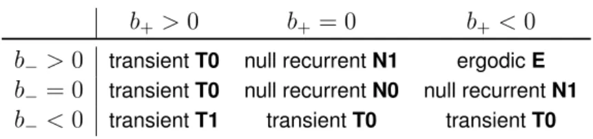
Therefore, the regimes of

ξ

depends only on the respective signs of

b

+and

b

−. Nine combinations are

possible. As some cases are symmetric, we actually consider five cases exhibiting different asymptotic behaviors of

Q

±_T, hence of the estimators. This is summarized in Table 2.

These cases are:

E) Ergodic case

b

+

<

0

,

b

−

>

0

.

N0) Null recurrent case

b

+

= 0

,

b

−

= 0

.

(8)

b

+

>

0

b

+

= 0

b

+

<

0

b

−

>

0

transientT0 null recurrentN1 ergodicE

b

−

= 0

transientT0 null recurrentN0 null recurrentN1

b

−

<

0

transientT1 transientT0 transientT0

Table 2: Recurrence and transience properties of

ξ

.

T0) Transient case

b

+

>

0

,

b

−

≥

0

.

T1) Transient case

b

+

>

0

,

b

−

<

0

.

CaseT0corresponds to two entries of table 2. The case

b

+

<

0

,

b

−

= 0

is symmetric toN1. Case

b

+

≤

0

,

b

−

<

0

is symmetric toT0.

4

Asymptotic behavior of the estimators

In this section, we state our main results on the asymptotic behavior of the occupation times of the process and the corresponding ones of the estimators, for each of the 5 cases.

Proposition 2(Ergodic caseE). If

b

+

<

0, b

−

>

0

, then

Q

+_T

T

,

Q

−_T

T

a.s.

−−−→

T→∞

|b

−

|

|b

−

|

+

|b

+

|

,

|b

+

|

|b

−

|

+

|b

+

|

.

(7) In addition,

(β

_T+

, β

_T−

)

−−−→

a.s. T→∞

(b

+

, b

−

)

and

√

T

p

|b

−

|

+

|b

+

|

(β

_T+

−

b

+

, β

T−

−

b

−

)

law

−−−→

T→∞

σ

+

p

|b

−

|

N

+

,

p

σ

−

|b

+

|

N

−

!

,

where

N

+_and

N

−_{are two independent, unit Gaussian random variables.}

Proposition 3(Null recurrent case with vanishing driftN0). Assume

b

+

=

b

−

= 0

. Assume

ξ

0

= 0

.

Then

Q

+_T

T

,

Q

−_T

T

law

= (Λ,

1

−

Λ)

for all

T >

0,

where

Λ

follows a law of arcsine type with density

p

Λ

(u) :=

1

π

1

p

u(1

−

u)

σ

+

/σ

−

1

−

(1

−

(σ

+

/σ

−

)

2

)u

for

0

< u <

1.

Besides,

√

T

(β

_T+

, β

_T−

)

law

= (β

₁+

, β

₁−

)

(8)

where the explicit joint density of

(β

₁+

, β

₁−

)

is given by (25)below. In particular,

(β

_T+

, β

_T−

)

converges almost surely to

(b

+

, b

−

) = (0,

0)

.

(9)

Proposition 4(Null recurrent case with non-vanishing driftN1). Assume

b

+

= 0

,

b

−

>

0

. Then

Q

+_T

T

a.s.

−−−→

T→∞

1

and

(β

+ T

, β

− T

)

a.s.

−−−→

T→∞

(b

+

, b

−

).

In addition, there exists three independent unit Gaussian random variables

N

−,

N

+and

N

such that

Q

−_T

√

T

,

√

T

(β

_T+

−

b

+

), T

1/4

(β

_T−

−

b

−

)

law

−−−→

T→∞

σ

+

b

−

|N |, σ

+

N

+

, σ

−

p

b

−

p

σ

+

·

N

−

p

|N |

!

.

(9)

Proposition 5(Transient case for upward driftT0). Assume

b

+

>

0

,

b

−

≥

0

so that the process

ξ

is

transient and

lim

T→∞

ξ

T

= +∞

. Then

Q

+_T

/T

1

as

T

→ ∞

and

β

_T+

−−−→

a.s. T→∞

b

+and

√

T

(β

_T+

−

b

+

)

law

−−−→

T→∞

σ

+

N

+ (10)

for a unit Gaussian random variable

N

+_{. Let}

`

0be the last passage time to

0

, which is almost surely

finite. Assume

ξ

0

= 0

. We have

β

_T−

1

T >`0

=

R

T0

1

T >`0 and

lim

T→∞

β

− T

=

R

T0a.s. with

R

T0

:=

L

∞

(ξ)

2Q

−_` 0

=

L

∞

(ξ)

2Q

− ∞

.

(11)

The density of

R

T0is given by (22)below. The case

b

+

≤

0

,

b

−

<

0

is treated by symmetry.

Proposition 6(Transient case for diverging driftT1). Assume

b

+

>

0

,

b

−

<

0

so that the process

ξ

is transient. Assume that

ξ

0

= 0

. Then there exists a Bernoulli random variable

B ∈ {0,

1}

such that

P

(B

= 1) = 1

−

P

(B

= 0) =

σ

−

b

+

σ

+

b

−

+

σ

−

b

+

,

P

+

Q

+_T

T

−−−→

T→∞

1

= 1

and

P

−

Q

−_T

T

−−−→

T→∞

1

= 1

with

P

+

(·) =

P

(· | B

= 1)

and

P

−

(·) =

P

(· | B

= 0).

On the event

{B

= 1}

(resp.

{B

= 0}

),

β

_T+(resp.

β

_T−) converges almost surely to

b

+(resp.

b

−) while

β

_T−

−

b

−(resp.

β

T+

−

b

+) is the ratio of two a.s. finite random variables.

In addition, for unit Gaussian random variables

N

+_and

N

−_,

√

T

(β

_T+

−

b

+

)

law

−−−→

T→∞

σ

+

N

+ under

P

+

,

(12)

√

T

(β

_T−

−

b

−

)

law

−−−→

T→∞

σ

−

N

− under

P

−

.

(13) In addition,

lim

T→∞

β

− T

=

R

−

T1a.s. under

P

+with

R

− T1

=

L

∞

(ξ)

2Q

− ∞

,

(14)

lim

T→∞

β

+ T

=

−R

+

T1a.s. under

P

−with

R

+ T1

=

L

∞

(ξ)

2Q

+ ∞

.

(15)

(10)

5

Auxiliary tools

In this section, we give first some results on a martingale central limit theorem that will be used con-stantly. To deal with the transient or null recurrent cases, we make use of some analytic properties of one-dimensional diffusions.

5.1

Limit theorems on martingales

The following result follows immediately from [32, Proposition 1, p. 148; Theorem 1, p. 150].

Proposition 7(A criterion for convergence). Under the true probability

P

,

(i) as

T

→ ∞

,

β

_T+ (resp.

β

_T−) converges a.s. to

b

+ (resp.

b

−) on the event

{Q

+∞

= +∞}

(resp.

{Q

−

∞

= +∞}

).

(ii) as

T

→ ∞

,

M

_T+ (resp.

M

_T−) converges a.s. to a finite value on the event

{Q

+

∞

<

+∞}

(resp.

{Q

−

∞

<

+∞}

). In other words,

β

±

T is not a consistent estimator on

{Q

±

∞

<

+∞}

.

We now state an instance of a Central Limit theorem for martingales which follows from [7]. This theorem will be used to deal with the casesE,N1andT1. Let us start by recalling the notion of stable convergence introduced by A. Rényi [21, 40].

Definition 1(Stable convergence). A sequence

(X

n

)

n∈Non a probability space

(Ω,

F,

P

)

is said to

converge stably with respect to a

σ

-algebra

G ⊂ F

if for any bounded, continuous function

f

and any bounded,

G

-measurable random variable

Y

,

E

(f(X

n

)Y

)

−−−→

n→∞

E

(f(X)Y

).

Proposition 8 (A central limit theorem for martingales). Let

(Ω,

F

,

P

)

be the underlying probability space of the process

ξ

with a filtration

(F

t

)

t≥0. If for some constants

c

+

, c

−

>

0

,

Q

+_T

T

P

−−−−→

T→+∞

c

+and

Q

−_T

T

P

−−−−→

T→+∞

c

−

,

then for the martingales

M

±defined in Lemma 1,

M

_T+

√

T

,

M

_T−

√

T

F∞−stably

−−−−−−→

T→∞

(σ

+

√

c

+

N

+

, σ

−

√

c

−

N

−

),

(16) on a probability space

(Ω

0

,

F

0

,

P

0

)

extending

(Ω,

F

,

P

)

and containing two independent unit Gaussian

random variables

N

+,

N

−, themselves independent from

ξ

. In addition,

√

T

M

_T+

Q

+_T

,

M

_T−

Q

−_T

F∞−stably

−−−−−−→

T→∞

σ

+

√

c

+

N

+

,

σ

−

√

c

−

N

−

,

(17) Proof. Set

a

T

:=

1/

√

T

0

1/

√

T

and

q

T

=

hM, M

i

_T

=

σ

2 +

Q

+ T

0

σ

2 −

Q

− T

.

Thus,

a

T

q

T

a

0T

=

"

σ

2 + Q+_T T

0

σ

2 − Q−_T T

#

P

−−−→

T→∞

c

+

c

−

.

(18)

(11)

Theorem 2.2 in [7] yields (16). Besides,

√

T

M

± T

Q

±_T

=

T

Q

±_T

×

M

_T±

√

T

.

(19)

If a sequence

(X

n

)

n converges

F

∞-stably and a sequence

(Y

n

)

n of

F

∞-measurable random

vari-ables converges in probability, then

(X

n

, Y

n

)

nconverges

F

∞-stably. Using the property in (19) and

(17) yields (17).

5.2

The fundamental system

Along with the characterization through the scale function and the speed measure, much information on the process can be read from the so-calledfundamental system[11, 19, 41]: For any

λ >

0

, there exists some functions

φ

λ and

ψ

λsuch that

ψ

λand

φ

λare continuous, positive from

R

to

R

with

φ

λ

(0) =

ψ

λ

(0) = 1

.

ψ

λis increasing with

lim

x→−∞

ψ

λ

(x) = 0

,

lim

x→∞

ψ

λ

(x) = +∞

.

φ

λis decreasing with

lim

x→−∞

φ

λ

(x) = +∞

,

lim

x→∞

φ

λ

(x) = 0

.

φ

λand

ψ

λare solutions to

Lf

=

λf

.

In the case of piecewise constant coefficients with one discontinuity at

0

, these solutions may be computed as linear combinations of the minimal functions for constant coefficients. Using the fact that

φ

,

φ

0,

ψ

and

ψ

0 are continuous at

0

,

ψ

λ

(x) =











exp

x

−b−+

√

b2 −+2σ2−λ σ2 −

if

x <

0

κ

+

exp

x

−b++

√

b2 ++2σ+2λ σ2 +

+

δ

+

exp

x

−b+−

√

b2 ++2σ2+λ σ2 +

if

x

≥

0,

(20)

φ

λ

(x) =











κ

−

exp

x

−b−−

√

b2 −+2σ2−λ σ2 −

+

δ

−

exp

x

−b−+

√

b2 −+2σ−2λ σ2 −

if

x <

0,

exp

x

−b+−

√

b2 ++2σ+2λ σ2 +

if

x

≥

0

(21) with

κ

+

:=

−b

−

σ

2+

+

b

+

σ

2−

+

σ

−2

p

b

2 +

+ 2λσ

+2

+

σ

2+

p

b

2 −

+ 2λσ

−2

2σ

2 −

p

b

2 +

+ 2λσ

+2

,

δ

+

:=

b

−

σ

2+

−

b

+

σ

−2

+

σ

−2

p

b

2 +

+ 2λσ

2+

−

σ

+2

p

b

2 −

+ 2λσ

2−

2σ

2 −

p

b

2 +

+ 2λσ

2+

,

κ

−

:=

−b

−

σ

2₊

+

b

+

σ

2−

−

σ

−2

p

b

2 +

+ 2λσ

2+

+

σ

+2

p

b

2 −

+ 2λσ

−2

2σ

2 +

p

b

2 −

+ 2λσ

−2

,

δ

−

:=

b

−

σ

2+

−

b

+

σ

−2

+

σ

−2

p

b

2 +

+ 2λσ

2+

+

σ

+2

p

b

2 −

+ 2λσ

−2

2σ

2 +

p

b

2 −

+ 2λσ

−2

.

We also define the quantities [37]

b

ψ(λ) :=

1

2

ψ

_λ0

(0)

ψ

λ

(0)

=

−b

−

+

p

b

2 −

+ 2σ

−2

λ

2σ

2 −

≥

0

and

φ(λ) :=

b

−

1

2

φ

0_λ

(0)

φ

λ

(0)

=

b

+

p

b

2 +

+ 2σ

+2

λ

2σ

2 +

≥

0.

(12)

In particular,

b

ψ(0) = 0

and

φ(0) =

b

+

σ

2 + when

b

−

≥

0

and

b

+

≥

0.

5.3

Last passage time and occupation time for the transient process

When

ξ

is a transient process, the last passage time

`

0

= sup{t

≥

0

|

ξ

t

= 0}

of

ξ

at

0

is almost

surely finite. Its Laplace transform is (See (53) in [37]):

E

0

[exp(−λ`

0

)] =

b

ψ(0) +

φ(0)

b

ψ(λ) +

φ(λ)

b

.

Let us now assume that

b

+

>

0

and

b

−

≥

0

. This is the transient caseT0where the process ends

up almost surely in the positive semi-axis. Thus,

Q

−_`

0

=

Q

−

∞and

L

`0

(ξ) =

L

∞

(ξ)

.

Let us write

b

±

:=

b

±

/σ

±2. From Corollary 5 in [37],

E

0

[exp(−αL

∞

(ξ)

−

λQ

−∞

)] =

b

ψ(0) +

φ(0)

b

α

+

φ(0) +

b

ψ(λ)

b

=

b

+

α

+

b

₊

−

bb− 2

+

1 2σ2 −

p

b

2 −

+ 2σ

−2

λ

.

Let

p

L∞(ξ)

(t)

be the density of

L

∞

(ξ)

. Setting

λ

= 0

, we see that

L

∞

(ξ)

is distributed according to

an exponential distribution of rate

b

₊. Thus,

p

_L_∞₍_ξ₎

(t) =

b

₊

exp(−

b

₊

t)

. A conditioning shows that

E

0

[exp(−αL

∞

(ξ)

−

λQ

−∞

)] =

Z

+∞ 0

exp(−αt)

E

0

exp(−λQ

−∞

)

L

∞

(ξ) =

t

p

L∞

(t) dt.

By inverting the Laplace transform with respect to

α

, since

p

L∞

(t) =

b

+

exp(−

b

+

t)

,

E

0

exp(−λQ

−∞

)

L

∞

(ξ) =

t

= exp

−t

−

b

−

2

+

1

√

2σ

−

s

b

2 −

2σ

2 −

+

λ

!!

.

Inverting the latter Laplace transform with respect to

λ

, the density

p

_Q−

∞

(s|t)

of

Q

− ∞given

{L

∞

(ξ) =

t}

is

p

_Q− ∞

(s|t) =

t

σ

−

2

√

2πs

3/2

exp

tb

−

2σ

2 −

−

b

2 −

s

2σ

2 −

−

t

2

8σ

2 −

s

.

Hence, the distribution

p

₍_Q−

∞,L∞(ξ))

(s, t)

of the pair

(Q

− ∞

, L

∞

(ξ))

is

p

₍_Q− ∞,L∞(ξ))

(s, t) =

tb

+

σ

2 +

σ

−

2

√

2πs

3/2

exp

b

−

2σ

2 −

−

b

+

σ

2 +

t

−

b

2 −

s

2σ

2 −

−

t

2

8σ

2 −

s

.

The density

p

RT0

(r)

of the random variable

R

T0

:=

L

∞

(ξ)/2Q

− ∞is then

p

RT0

(r) = 2

Z

+∞ 0

s

·

p

₍_Q− ∞,L∞(ξ))

(s,

2rs) ds

=

rb

+

σ

2 +

σ

−

√

2

2rb

+

σ

2 +

+

(r

−

b

−

)

2

2σ

2 −

−3/2

, r >

0.

(13)

The distribution of

L

∞

(ξ)/2Q

+∞when

b

−

<

0

,

b

+

≤

0

is found by symmetric arguments.

Let us now assume that

b

+

>

0

and

b

−

<

0

. This is the transient caseT1where the process can end

up in both semi-axis. The Laplace transform is

E

0

[exp(−αL

∞

(ξ)

−

λQ

−∞

)] =

b

ψ(0) +

φ(0)

b

α

+

φ(0) +

b

ψ(λ)

b

=

b

+

−

b

−

α

+

b

₊

−

bb− 2

+

1 2σ2 −

p

b

2−

+ 2σ

−2

λ

.

With analogous computations as before we get that the density

p

_R−

T1

(r)

of

R

− T1is

p

_R− T1

(r) =

r

σ

−

√

2

b

+

σ

2 +

−

b

−

σ

2 −

2rb

+

σ

2 +

+

(r

−

b

−

)

2

2σ

2 −

−3/2

, r >

0.

Considering also the previous case, we can write the following formula, holding for the density of

R

=

R

T0or

R

=

R

−_T1in both casesT0andT1:

p

R

(r) =

r

σ

−

√

2

b

+

σ

2 +

+

L

b

−

M

−

σ

2 −

2rb

+

σ

2 +

+

(r

−

b

−

)

2

2σ

2 −

−3/2

, r >

0.

(22)

Notice that this is the density of a positive random variable which is not integrable. This gives the limit behavior of the estimator

β

_T−of

b

−. The behavior of

β

_T+ in the corresponding cases can be found by

symmetric arguments.

6

Proofs of the asymptotic behavior of the estimators

6.1

Asymptotic behavior for the ergodic case (E)

The ergodic case is the most favorable one. The process

ξ

is ergodic, so that for any bounded, mea-surable function

f

, _T1

R

₀T

f

(ξ

s

) ds

R

f(x)

_Mm(₍x)

R)

dx

.

With the explicit expression of

M

that follows from (6),

M

(

R

+

) =

−1

b

+

, M

(

R

−

) =

1

b

− and

M(

R

) =

|b

+

b

−

|

|b

−

|

+

|b

+

|

.

From the ergodic theorem, since

Q

±_t

=

R

₀t

1

±ξs≥0

ds

,

Q

±_T

T

a.s.

−−−→

T→∞

M

(

R

±

)

M

(

R

)

so that

Q

+_T

T

a.s.

−−−→

T→∞

|b

−

|

|b

−

|

+

|b

+

|

and

Q

− T

T

a.s.

−−−→

T→∞

|b

+

|

|b

−

|

+

|b

+

|

.

(23)

(14)

6.2

Asymptotic behavior for the null recurrent case with vanishing drift (N0)

When

b

−

=

b

+

= 0

, the process

ξ

is an Oscillating Brownian motion (OBM, introduced first in [24],

0

,

L

ξ

T

M

+

√

T

,

L

ξ

T

M

−

√

T

,

L

T

(ξ)

√

T

,

Q

+_T

T

law

= (

L

ξ

1

M

+

,

L

ξ

1

M

−

, L

1

(ξ), Q

+1

).

Therefore,

√

T

β

_T+

β

_T−

=







L

ξ

T

M

+

/

√

T

−

1 2

L

T

(ξ)/

√

T

Q

+_T

/T

1 2

L

T

(ξ)/

√

T

−

L

ξ

T

M

−

/

√

T

Q

−_T

/T







law

=

β

₁+

β

₁−

=







L

ξ

1

M

+

−

1 2

L

1

(ξ)

Q

+₁ 1 2

L

1

(ξ)

−

L

ξ

1

M

−

Q

−₁







.

We recall now that

X

= Φ(ξ) :=

ξ/σ(ξ)

is a Skew Brownian motion [10, 30]. An explicit formula for the density for the position a Skew Brownian motion, its local time and its occupation time is known [2, 12]. Since the transform

Φ

is piecewise linear, one easily recover the one of an OBM, its local and occupation times. Hence, the density of

(ξ

1

, L

1

(ξ), Q

+1

(ξ))

is

p

₍_ξ 1,L1(ξ),Q+1)

(ρ, λ, τ

)

=











(λ/2 +

ρ)λ/2

2πσ

−

σ

3+

(1

−

τ)

3/2

τ

3/2

exp

−

(λ/2)

2

2σ

2−

(1

−

τ

)

−

(λ/2 +

ρ)

2

2σ

2₊

τ

for

ρ

≥

0,

(λ/2

−

ρ)λ/2

2πσ

+

σ

3−

(1

−

τ)

3/2

τ

3/2

exp

−

(λ/2)

2

2σ

2 +

τ

−

(λ/2

−

ρ)

2

2σ

2 −

(1

−

τ

)

for

ρ <

0.

(24)

The change of variable in the density suggested by

(β

₁+

, β

₁−

, Q

+₁

) =

L

ξ

1

M

+

−

L

1

(ξ)/2

Q

+₁

,

L

1

(ξ)/2

−

L

ξ

1

M

−

1

−

Q

+₁

, Q

+ 1

gives

p

₍_β+ 1,β − 1,Q + 1)

(a, b, δ)

= 2δ(1

−

δ)p

₍_ξ

1,L1(ξ),Q+1)

(aδ

+

b(1

−

δ),

|aδ

+

b(1

−

δ)| −

aδ

+

b(1

−

δ), δ)

and then, since

Q

+₁

∈

[0,

1]

,

p

₍_β+ 1,β − 1)

(a, b)

=

Z

1 0

2δ(1

−

δ)p

₍_ξ

1,L1(ξ),Q+1)

(aδ

+

b(1

−

δ),

|aδ

+

b(1

−

δ)| −

aδ

+

b(1

−

δ), δ) dδ.

(25)

6.3

Asymptotic behavior for the null recurrent case with non-vanishing drift

(N1)

We consider

b

+

= 0

,

b

−

>

0

. The particle is then pushed upward when its position is negative. Yet

the process is only null recurrent. The measure

M

satisfies

M

(

R

−

) =

1

b

−

(15)

Using 9) in [19, Section 6.8, p. 228] or [34, 47], with (26),

Q

−_T

T

a.s.

−−−→

T→∞

M

(

R

−

)

M

(

R

)

= 0.

Since

Q

+_T

+

Q

−_T

=

T

, it holds that

Q

+_T

/T

1

. Using Proposition 8 on

M

+_{only, we obtain that}

M

_T+

√

T

law

−−−→

T→∞

σ

+

N

+ (27)

for a Gaussian random variable

N

+

∼ N

(0,

1)

and then that

√

T

(β

_T+

−

b

+

)

law

−−−→

T→∞

σ

+

N

+_.

The asymptotic behavior of

Q

−_T is more delicate to deal with as the process

ξ

is only null recurrent. For this, we use the results of [14] which extends the one of D.A. Darling and M. Kac [8] on additive and martingale additive functionals.

The Green kernel with respect to the invariant measure

M

of

L

is given by [11, 19, 41]

g

λ

(x, y) :=

1

W

λ

(

ψ

λ

(x)φ

λ

(y)

if

x < y,

φ

λ

(x)ψ

λ

(y)

if

x

≥

y

with

W

λ

=

ψ

_λ0

(0)φ

λ

(0)

−

ψ

λ

(0)φ

0λ

(0)

S

0

(0)

.

The Wronskian

W

λis then equal to

W

λ

=

√

2λ

σ

+

p

b

2 −

+ 2λσ

2−

σ

−2

−

b

−

σ

2−

.

In particular,

W

λ

/

√

λ

converges to

√

2/σ

+as

λ

converges to

0

.

On the other hand, it follows from (20) and (21) that

ψ

λ

(x)

−−→

λ→0

ψ

0

(x) := 1

and

φ

λ

(x)

−−→

λ→0

φ

0

(x) := 1

when

x >

0

while

ψ

λ

(x) = exp(x

√

2λ)

−−→

λ→0

ψ

0

(x) := 1

and

φ

λ

(x) =

φ

0

(x) := 1

when

x

≥

0.

For a measurable function

f

:

R

→

R

+ such that

R

f

dM <

+∞

, the above convergence results imply that

√

λ

Z

R

g

λ

(x, y)f

(x)m(y) dy

−−→

λ→0

σ

+

√

2

Z

R

f

(y)m(y) dy,

∀x

∈

R

.

We then define

`(λ) :=

√

2/σ

+which is a constant function, and

α

:= 1/2

, the exponent of

λ

.

Let

(M

t

)

t≥0 be a Mittag-Leffler process of index

1/2

(it is the inverse of an increasing stable process

of index

1/2

). The process

2

−1/2

M

is equal in distribution to the running maximum of a Brownian motion, or equivalently, to the local time of a Brownian motion [14, Remark 2.9, p. 21].

From Theorem 3.1 and Corollary 3.2 in [14, p. 26], since

hM

−

i

_t

=

σ

2 −

Q

− t,

t

≥

0

and

M

is continu-ous,

p

`(n)

M

− nt

n

1/4

, `(n)

Q

−_nt

√

n

t∈[0,1] law

−−−→

n→∞

σ

−

√

νB

−

(M

t

), νM

t

t∈[0,1] (28)

(16)

with respect to the uniform topology, where

B

is a Brownian motion independent from

M

and

ν

=

Z

R

m(y)

E

y

Z

1 0

1

ξs≤0

ds

dy

=

M

(

R

−

) =

1

b

−

.

From the reflection principle, the distribution of

M

1 is the same as the one of a truncated normal

distribution

√

2T

where

T

:=

|G|

with

G ∼ N

(0,

1)

. Setting

t

= 1

in (28) and using the scaling property of the Brownian motion

B

−,

M

_T−

T

1/4

,

Q

−_T

T

1/2

law

−−−→

T→∞

σ

−

√

σ

+

p

b

−

√

T · N

−

,

σ

+

b

−

T

!

for a Gaussian random variable

N

−

∼ N

(0,

1)

independent from

T

. It remains to show the independence of

N

+_,

N

−_and

T

_.

Since

hM

±

i

t

=

σ

2 ±

Q

±

t and

hM

+

, M

−

i

t

= 0

for any

t

≥

0

, the Knight theorem [18,

Theo-rem 7.3’, p. 92] implies that there exists on an extension of

(Ω,

F

,

P

)

a

2

-dimensional Brownian motion

(B

+

, B

−

)

such that

M

_t±

=

B

±

(σ

2 ±

Q

±

t

)

for any

t

≥

0

. Let us set

B

n+

(t) =

n

−1/2

B

+

(nt)

and

B

_n−

(t) =

n

−1/4

B

−

(

√

nt)

for any integer

n

and any

t

≥

0

. From the scaling property,

(B

+_n

, B

_n−

)

is still a

2

-dimensional Brownian motion which converges in distribution to a

2

-dimensional Brownian motion

(B

+

∞

, B

∞−

)

in the space

C

([0,

1],

R

2

)

of continuous functions.

For any

0

≤

s

≤

t

≤

1

,

Q

+_nt

−

Q

+

ns

≤

n(t

−

s)

so that

(Q

+

nt

/n)

t∈[0,1] is tight in the space of

continuous functions. Hence,

(Q

+_nt

/n)

t∈[0,1]converges in probability to the identity map

t

7→

t

in the

space of continuous function

C([0,

1],

R

)

.

Combining this result with (28), it holds that

B

_n+

(t), B

_n−

(t), n

−1

Q

+_nt

, n

−1/2

Q

−_nt

_t∈_[0_,_1] is tight in

C

([0,

1],

R

4

)

and then necessarily

B

_n+

(t), B

_n−

(t),

Q

+ nt

n

,

Q

−_nt

√

n

t∈[0,1] law

−−−→

n→∞

(B

+ ∞

(t), B

− ∞

(t), t, νM

t

)

t∈[0,1]

in the space of continuous functions

C

([0,

1],

R

4

)

_{. Being the inverse of a}

1/2

_{-stable process, hence}

a pure jump process,

M

is independent from

(B

+

∞

, B

∞−

)

for the arguments presented in [14, p. 38]

or [18, Theorem 6.3, p. 77]. For any

t

∈

[0,

1]

, it holds that

M

_nt+

√

n

=

1

√

n

B

+

(σ

2 +

Q

+ nt

) =

B

+ n

σ

2₊

Q

+ nt

n

and

M

− nt

n

1/4

=

1

√

n

B

−

(σ

₋2

Q

−_nt

) =

B

_n+

σ

₋2

Q

+ nt

√

n

.

Using

(n

−1

Q

+

nt

)

t∈[0,1] and

(n

−1/2

Q

−nt

)

t∈[0,1] as random time changes, we deduce from the results

in [5, p. 144] that

M

_nt+

n

1/2

,

M

_nt−

n

1/4

,

Q

+_nt

n

,

Q

−_nt

√

n

t∈[0,1] law

−−−→

n→∞

(B

+

(σ

2 +

t), B

−

(σ

₋2

νM

t

), t, νM

t

)

t∈[0,1]

.

By setting

N

+

:=

B

+

(σ

2 +

)/σ

+in (27),

T

:=

M

1

/

√

2

and

N

−

:=

B

−

(σ

2 −

ν)/σ

−

√

ν

, this proves (9) using

t

= 1

in the above limit.

(17)

6.4

Asymptotic behavior for the transient case (T0)

We recall that we consider only

b

+

>

0

and

b

−

≥

0

.

It is known that the last passage time

`

0 to

0

is almost surely finite so that

Q

−∞

<

∞

almost surely.

Since

Q

+_T

=

T

−

Q

_T−, we obtain that

Q

+_T

/T

1

. The convergence results regarding

β

_T+follows from Proposition 8 applied only to one component.

The asymptotic behavior of

β

_T+follows from Proposition 7(ii).

When

T > `

0 and

ξ

0

= 0

, then

ξ

T

>

0

and thus

β

T−

=

L

T

(ξ)/2Q

−T. Yet the local time

L

T

(ξ)

and the occupation times

Q

−_T are constant when

T > `

0. The result follows by the computations of

Section 5.3.

6.5

Asymptotic behavior for the transient case generated by diverging drift

(T1)

When

b

−

<

0

and

b

+

>

0

, the process is also transient as

S(+∞)

<

+∞

and

S(−∞)

>

−∞

. The scale function

S

map

R

to

(−γ

−

, γ

+

)

with

γ

±

=

|σ

±2

|2b

±. From the Feller test [23,

Theorem 5.29], the process does not explode. Thus, as

ξ

0

= 0

, it follows from [48] or [23, Proposition

5.5.22, p. 354] that

p

:=

P

lim

T→∞

ξ

T

= +∞

= 1

−

P

lim

T→∞

ξ

T

=

−∞

=

γ

−

γ

−

+

γ

+

=

σ

2 −

b

+

σ

2 +

b

−

+

σ

−2

b

+

.

Then event that

{lim

T→∞

|ξ

T

|

= +∞}

arise when the process starts an excursion with infinite

lifetime, thus after the last passage time to

0

. We denote by

A

±the event

{lim

T→∞

Q

±_T

/T

= 1}

, so

that

A

+

∩

A

−

=

∅

. Hence,

P

(A

+

) = 1

−

P

(A

−

) =

p

.

Using the same arguments as in the case T0, given

A

±,

β

_T± converges almost surely to

b

± while

β

_T∓

=

±L

∞

(ξ)/Q

∓_`₀.

For the Central Limit Theorem, we apply Corollary 2.3 in [7] on

M

_T+

/

√

T

. As

Q

+_T

>

0

a.s. as soon as

T >

0

since

ξ

0

= 0

and

{B

=

p}

=

A

+

,

a.s. for

p

= 0,

1,

it follows that for a normal distribution

N

,

s

T

σ

2 +

Q

+T

·

M

√

T

F∞−stably

−−−−−−→

N→∞

N

under

P

(· | B

= 1).

It follows that

β

_T+

−

b

+

=

√

T

M

T

Q

+_T

=

σ

+

s

T

Q

+_T

s

T

σ

2 +

Q

+T

M

T

√

T

F∞−stably

−−−−−−→

N→∞

σ

+

N

under

P

(· | B

= 1).

Hence the result.

7

Wilk’s theorem and LAN property

Owing to the quadratic nature of the log-likelihood, we easily deduce both a Wilk theorem, on which a hypothesis test may be developed, as well as the Local Asymptotic Normality (LAN) property, which

(18)

proves that our estimators are asymptotically efficient.

7.1

Wilk’s theorem and a hypothesis test

The log-likelihood

log

G(b

+

, b

−

)

can be computed from the data using (5). Moreover, this function is

quadratic in

b

+and

b

−. We have then

D(b

+

, b

−

) :=

∇

log

G(b

+

, b

−

) =





LξTM + σ2 +

−

Lξ0M + σ2 +

−

1 2σ2 +

L

T

(ξ)

−

b+ σ2 +

Q

+ T

−

LξTM − σ2 −

+

Lξ0M − σ2 −

+

1 2σ2 −

L

T

(ξ)

−

b− σ2 −

Q

− T





and

H(b

+

, b

−

) := Hess log

G(b

+

, b

−

) =





−

Q+T σ2 +

0

−

Q−T σ2 −





.

Therefore, around any point

(b

+

, b

−

)

,

log

G(b

+

+ ∆b

+

, b

−

+ ∆b

−

) = log

G(b

+

, b

−

)

+

D(b

+

, b

−

)

·

∆b

+

∆b

−

Q

+ T

2σ

2 +

∆b

2₊

−

Q

− T

2σ

2 −

∆b

2₋

.

(29)

In particular, we prove a result in the asymptotic behavior of the log-likelihood for the ergodic caseEor the null recurrent caseN1. A similar result can be given for the null recurrent casesN0with a different limit distribution that can be identified with the density given in Section 6.2.

Proposition 9(Wilk’s theorem; Ergodic caseEor null recurrent caseN1). Denote by

(b

true

+

, b

true−

)

be

the real parameters. Then

−2 log

G(b

true₊

, b

true₋

)

−−−→

law

T→∞

χ

2

:= (N

+

)

2

+ (N

−

)

2under

P

₍_btrue

+ ,btrue− ) (30)

for two independent, unit Gaussian random variables

N

+ _and

N

−_{. Besides, when}

(b

+

, b

−

)

6=

(b

true +

, b

true−

)

, then

−

log

G(b

+

, b

−

)

a.s.

−−−→

T→∞

+

∞

under

P

(b true + ,btrue− )

.

(31)

Proof. Considering (29) at

(b

+

, b

−

) = (β

_T+

, β

_T−

)

since

D(β

_T+

, β

_T−

) = (0,

0)

, for any parameter

(b

+

, b

−

)

and any

α

+

, α

−

>

0

,

log

G(b

+

, b

−

) =

−

Q

+_T

2T

α+

σ

2 +

T

α₊ 2

(b

+

−

β

T+

)

2

−

Q

− T

2T

α−

σ

2 −

T

α− 2

(b

₋

−

β

− T

)

2

.

When the process is ergodic (CaseE), we set

(α

+

, α

−

) = (1,

1)

. It follows from Proposition 2 that

(30) holds. When

(b

+

, b

−

)

6= (b

true₊

, b

true−

)

, then

β

±

T

−

b

±does not converge to

0

while

Q

+

T converges

a.s. to infinity. This proves (31). The result is similar in the caseN1with

(α

+

, α

−

) = (1,

1/2)

.

A hypothesis test can be developed from Proposition 9. The null hypothesis is

(b

+

, b

−

) = (b

0+

, b

0−

)

for a given drift

(b

0

+

, b

0−

)

while the alternative hypothesis is

(b

+

, b

−

)

6= (b

0₊

, b

0−

)

.

Using (5), we compute

log

G(b

0

+

, b

0−

)

. The null hypothesis is rejected with a confidence level

α

if

−

log

G(b

0

+

, b

0−

)

> q

αwhere

q

αis the

α

-quantile

P

[χ

2

≤

q

α

] =

α

while

χ

2 follows a

χ

2distribution

(19)

7.2

The LAN property

The LAN (local asymptotic normal) property, introduced by L. Le Cam in [29], characterizes the effi-ciency of the estimator (See also [16,27] among many other references). It was extended as the LAMN (local asymptotic mixed normal) to deal with a mixed normal limits by P. Jeganathan in [22].

The quadratic nature of the log-likelihood as well as our limit theorems implies that the LAN (resp. LAMN) property is verified in the ergodic caseE(resp. null recurrent caseN1).

Proposition 10(LAN property; Ergodic case E). In the ergodic caseE, the LAN property holds for the likelihood at

(b

true

+

, b

true−

)

with rate of convergence

(σ

2+

/

√

T , σ

2

−

/

√

T

)

and asymptotic Fisher information

Γ :=

1

|b

−

|

+

|b

+

|

σ

2 +

|b−|

0

σ

2 −

|b+|

.

Proof. At

(b

true₊

, b

true₋

)

, the gradient may be written

D(b

true₊

, b

true₋

) =





Q+_T √ T σ2 +

√

T

(β

_T+

−

b

true +

)

Q−_T √ T σ2 −

√

T

(β

_T−

−

b

true −

)





.

Using (29),

R(T

) := log

G

b

true +

+

σ

+2 ∆_√b+ T

, b

true −

+

σ

2− ∆_√b− T

G(b

true +

, b

true−

)

=

Q

+_T

(β

_T+

−

b

true₊

)

Q

−_T

(β

_T−

−

b

true −

).

·

∆b

+

∆b

−

σ

2 +

Q

+ T

2T

∆b

2 +

−

σ

2 −

Q

− T

2T

∆b

2 −

=

√

1

T

M

_T+

M

_T−

·

∆b

+

∆b

−

1

2T

∆b

+

∆b

−

· hM

+

, M

−

i

T

∆b

+

∆b

−

(32)

With

c

=

|b

+

|

+

|b

−

|

, Proposition 2 implies that

(T

−1/2

M

+

,

−1/2

M

−

)

converges in distribution to

G ∼ N

(0,

Γ)

and

T

−1

hM

+

, M

−

i

T converges to the diagonal, definite positive matrix

Γ

. This proves

the LAN property.

Proposition 11 (LAMN property; Null recurrent caseN1). In the null recurrent caseN1, the LAMN property holds for the likelihood at

(b

true

+

, b

true−

)

with rate of convergence

(σ

+2

/T

1/2

, σ

−2

/T

1/4

)

and

asymptotic (random) Fisher information

Γ :=

σ

2 +

0

σ

2 − σ+ b−

|N |

for a normal random variable

N ∼ N

(0,

1)

.

8

Simulation study

8.1

From continuous to discrete data

In this section, we apply the estimator (4) to simulated processes. We test whether the results are good or not depending on sign and magnitude of involved quantities (cf. [36, Section 4.1]).

(20)

Estimator (4) involves

(ξ

0

, ξ

T

)

which are observable, as well as

(L

T

(ξ), Q

−T

, Q

+

T

)

which are not.

Imagine that we observe

ξ

t on a discrete time grid

{kT /n;

k

= 0, . . . , n}

. The time step between

two observations is

∆t

=

T /n

. In [30] we discuss, in the case of the Oscillating Brownian Motion, the estimator for the occupation time

Q

+_T given the Riemann sums:

b

Q

+_{T ,n}

= ∆t

n

X

k=1

1

ξkT /n≥0

.

We proved that the speed of convergence is strictly better than

√

n

, meaning that

√

n(

Q

b

+_{T ,n}

−

Q

+_T

)

−−−→

P

n→∞

0

. This result can be extended to the drifted process

ξ

via the Girsanov theorem.

Again in [30], we propose the following approximation of the local time of

ξ

at

0

b

L

T ,n

=

−3

2

r

π

2∆t

σ

+

σ−

σ

+

σ

− n

X

k=1

L

ξ

kT /n

M

+

−

L

ξ

(k−1)T /n

M

+

·

L

ξ

kT /n

M

−

L

ξ

(k−1)T /n

M

−

.

(33)

Up to some constants, this is essentially an approximation of the covariation between

L

ξ

t

M

+

and

L

ξ

t

M

−

. In [30] we also proved the consistence of such estimator. For the Brownian motion, this estimator converges at speed

n

1/4. The proof has not been adapted to our case because of the technical difficulties due to the discontinuity of the coefficients in

0

. Anyway we conjecture a rate of

1/4

. An alternative estimator can be constructed counting the number of crossings, as in [20]. We use (33) for empirical reasons, since it performs better on simulated trajectory.

At this point, we also notice that estimator (33) involves

σ

±, which are quantities not directly observable

on the trajectory; let us mention that the same is true for the classic estimator of local time for SDEs with differentiable coefficients [20]. Therefore, if

σ

±are known a priori, (33) can be implemented using

such quantities. Otherwise,

σ

±must be estimated on discrete time observations of

ξ

as well, a problem

which has been thoroughly investigated in [31].

We do not push further in the present paper the theoretical discussion on the quality of these dis-crete time approximations. Some more insights, based on numerical results, are given in the following section.

8.2

Implementation and simulation

The aim of the following section is to show on figures the numerical evidence of the central limit theorems stated in Section 4. We also mean to say something more on the choice of the step of the time grid in relation to the quality of the estimation of the local time. The code used for the following simulations have been implemented using the software

R

. We will consider time grids of the type

{0, T /N,

2T /N, . . . , T

} ⊂

N

, so with

N

∈

N

, and use as approximation of local and occupation time the following:

b

L

T ,N and

Q

b

+_T

:=

Q

b

+_T,N

.

Summing up, as estimators of

b

±we use the approximation

b

±_{T ,N}

=

±

L

ξ

T

M

±

−

L

ξ

0

M

±

−

L

b

_{T ,N}

/2

b

Q

±_T,N

.

(34)

(21)

These are our discrete times approximations of the continuous time estimators for which the conver-gence results have been proved. In practice, in some cases the estimator does not really depend on the local time, but is essentially determined by the final value of the process and the occupation times. In those cases, the quality of the discrete time approximation of the local time does not really matter, and therefore we can take

N

= 1

. In most cases, anyway, a good approximation of the local time is needed in order to observe on simulations the theoretical central limit behavior expected from Section 4. In these cases

N

∈

N

must be taken large enough.

In what follows, the choice of the parameters is detailed for every figure. The diffusion parameter is taken constant

σ

+

=

σ

−

= 0.01

, the same one for all the different simulations, and supposed known

a priori. In such manner the CLTs that we want to test can be better observed. To use estimator (34) on real data, with

σ

± not known, one must first use the estimators for

σ

±in [31] and then use such

estimations in the estimator (33) for the local time. We indicate with

[+]

and

[−]

estimation on positive and negative semiaxis, e.g.(N1)[+]stands for “estimation of

b

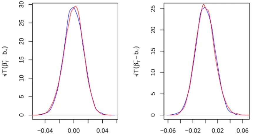
+” in caseN1.

−0.04 0.00 0.04 0 5 10 15 20 25 30 (E)[+] T ( βT +− b+ ) −0.06 −0.02 0.02 0.06 0 5 10 15 20 25 (E)[−] T ( βT −− b− )

Figure 1: (E). SDE parameters:

σ

±

= 0.01, b

−

=

0

.

004

, b

+

=

−

0

.

003. Simulation parameters:

T

=

1000

, N

=

100 000. We show both sides (positive and negative) of the estimation, displaying

the density of

√

T

(β

_T±

−

b

±

)

. The CLT in Proposition (7) is accurate for large

T

and time step

T /N

small, since the quality of the estimation of the local time is key in this case. The limit behavior is Gaussian.

(22)

−0.04 −0.02 0.00 0.02 0.04 0 10 20 30 40 (N1)[+] T ( βT +− b+ ) −0.04 −0.02 0.00 0.02 0.04 0 10 20 30 40 (T0)[+] T ( βT +− b+ ) −0.04 −0.02 0.00 0.02 0.04 0 10 20 30 40 (T1)[+] wrt P+ T ( βT +− b+ ) −0.04 −0.02 0.00 0.02 0.04 0 10 20 30 40 (T1)[−] wrt P− T ( βT −− b− )

Figure 2:(N1)[+],(T0)[+],(T1)[+]w.r.t

P

+,(T1)[−]w.r.t

P

−. SDE parameters:

σ

±

=

0

.

01; in case

N1:

b

−

=

0

.

004

, b

+

= 0;

in caseT0:

b

−

=

0

.

004

, b

+

=

0

.

006; in case

T1:

b

−

=

−

0

.

004

, b

+

=

0

.

003. Simulation parameters:

T

=

1000

, N

=

1000. We display the density of

√

T

(β

_T+

−

b

+

)

in

casesN1andT0. We also show

√

T

(β

_T±

−

b

±

)

in caseT1, but the density is w.r.t

P

± (cf. (6)). This

is approximated computing the estimator on trajectories such that

ξ

T is larger or respectively smaller

than

0

. In all these cases the CLT is Gaussian and we do not need to have a fine discretisation/time grid, since the local time is asymptotically negligible and the quantities which matter in the estimator are

ξ

T and the occupation times. This accounts of (9)-positive part, (10), (12) and (13).

−0.04 −0.02 0.00 0.02 0.04 0 10 20 30 40 50 (N1)[−] T ( 1 4 ) (β T − − b− )

Figure 3: (N1)[−]. SDE parameters:

σ

±

= 0.01;

in case N1:

b

−

=

0

.

004

;

b

+

= 0.

Simulation

parameters:

T

=

1000

, N

=

100 000. The CLT in (9)-negative part, is accurate for large

T

and time step

T /N

small, since the quality of the estimation of the local time is key in this case. Remark that in this case (null recurrent), the CLT has speed of convergence

T

1/4 and the limit law is not Gaussian. This accounts of (9)-negative part.

(23)

0.00 0.01 0.02 0.03 0.04 0.05 0 20 40 60 80 (T0)[−] βT − 0.00 0.01 0.02 0.03 0.04 0.05 0 5 10 15 20 25 30 (T1)[+], wrt P− βT + 0.00 0.01 0.02 0.03 0.04 0.05 0 10 20 30 40 50 60 70 (T1)[−], wrt P+ − βT −

Figure 4: (T0)[−], (T1)[+] w.r.t to

P

− and (T1)[−] w.r.t to

P

+. SDE parameters:

σ

±

= 0.01

; in

case T0:

b

−

=

0

.

004

, b

+

=

0

.

003; in case

T1:

b

−

=

−

0

.

003

, b

+

=

0

.

01. In case

T0: simulation

parameters:

T

=

20

, N

=

1000. We display the density of

β

_T−. In caseT1: simulation parameters:

T

=

20

, N

= 3

×10

7_{. We display the density of}

β

±

T w.r.t

P

∓(cf. (6)). This is approximated computing

the estimator on trajectories such that

ξ

T is smaller or respectively larger than

0

. In these cases

the estimator is not consistent, so what we show is not actually a CLT but the convergence of the estimators towards the law (22) (cf. results (11), (14), (15)). This convergence is accurate for large

T

but also depends on the time step

T /N

. Moreover, we see that the theoretical distribution of

β

_T− in case T1is almost singular at the origin, and therefore the exact behavior near the origin is hard to catch on simulated trajectories. This can be improved using different kernels (instead of the Gaussian one) in the estimation of the density. This can be easily done with the function “density” in

R

. The limit behavior is better approximated when

b

+ and

b

− have similar magnitude. We chose here to display

the case

b

−

=

−

0

.

003

;

b

+

=

0

.

01

to mention this critical behavior. Anyway, this feature does not

really matter in statistical application, because in this case the estimator not only is not consistent, but does not even guess the correct sign of the parameter. Indeed, we are here in the very critical case of a transient process generated by diverging driftT1.

(24)

−0.3 −0.2 −0.1 0.0 0.1 0 5 10 15 20 25 (N0)[+] T βT + −0.1 0.0 0.1 0.2 0.3 0 5 10 15 20 (N0)[−] T βT −