Wavelet regression using a Lévy prior model

Model

A thesis presented for the degree of

Doctor of Philosophy of the Diploma of Imperial College by

Badr Missaoui

MAY 17, 2013

2

I certify that this thesis, and the research to which it refers, are the product of my own work, and that any ideas or quotations from the work of other people, published or otherwise, are fully acknowledged in accordance with the standard referencing practices of the discipline.

Copyright

Copyright in text of this thesis rests with the Author. Copies (by any process) either in full, or of extracts, may be madeonlyin accordance with instructions given by the Author and lodged in the doctorate thesis archive of the college central library. Details may be obtained from the Librarian. This page must form part of any such copies made. Further copies (by any process) of copies made in accordance with such instructions may not be made without the permission (in writing) of the Author.

The ownership of any intellectual property rights which may be described in this thesis is vested in Imperial College, subject to any prior agreement to the contrary, and may not be made available for use by third parties without the written permission of the University, which will prescribe the terms and conditions of any such agreement. Further information on the conditions under which disclosures and exploitation may take place is available from the Imperial College registry.

4

Abstract

This thesis is concerned with nonparametric regression and regularization. In particular, wavelet regression using a Lévy prior model is investigated. The use of this prior is motivated by the statistical properties, such as heavy-tails, common in many datasets of interest, such as those in financial time series.

The Lévy process we propose captures the heavy tails of the wavelet coefficients of an unknown function. We study the Besov regularity of the wavelet coefficients and establish the connection between the parameters of the Lévy wavelet prior model and Besov spaces. At first, we gave a necessary and sufficient condition such that the realizations of the prior model fall into a certain class of Besov spaces. We show that the tempered stable distribution preserves its functional form for different time scales. We prove that this scaling behaviour can model the exponential-decay-across-scale property of the wavelet coefficients without imposing any specified structure on the coefficients’ energy.

We also introduce a Lévy wavelet mixture model to capture the sparseness of the wavelet coefficients. We show that this sparse model exhibits a thresholding rule. We also study the Lévy tempered stable prior model under a Bayesian framework. For the prior specified, we gave a closed form to the posterior Lévy measure of the wavelet coefficients and estimate the hyperparameters of the prior model in both a simulation study and for the S&P 500 time series.

We focus on density estimation using a penalized likelihood approach. Primarily, we study the wavelet Tsallis entropy and Fisher information and give closed-form expressions for these measures when the wavelet coefficients are driven by a tempered stable process. Then, we develop an entropic regularization based on the wavelet

6 Tsallis entropy and show that the penalized maximum likelihood method improves the convergence of the estimates.

Acknowledgements

I would like to thank Dr Emma McCoy for supervising this thesis. Working in the area of wavelet and nonparametric estimation has been a true learning experience for me and I am immensely grateful for the help my supervisor have given me. I also want to record a debt of gratitude to Prof. Nick Bingham for his comments, insights, and discussions. Lastly, thanks to Chris Minas for his help, discussions and fun times. Badr Missaoui

8

Contents

3.2.1 Fourier Transform and Regularity . . . 31

3.2.2 Short-Time Fourier Transform . . . 32

3.3 Wavelet Transform . . . 34

3.4 Continuous Wavelet Transform . . . 34

3.4.1 Regularity . . . 38

3.4.2 Hardy Spaces . . . 40

3.5 Multiresolution Analysis . . . 42

3.5.1 Theoretical framework . . . 43

3.6 Discrete Wavelet Transform . . . 47

3.7 Besov spaces . . . 50

3.8 Summary . . . 54

4 Basics on Lévy processes 55 4.1 Definitions . . . 55

4.2 Subordinators . . . 61

4.3 Stable processes . . . 62

4.4 Stochastic Integral representation for Stable Processes . . . 68

4.5 Tempered stable process . . . 68

4.7 Wiener Hopf Factorization . . . 73

4.8 Simulation of tempered stable processes . . . 76

4.9 Summary . . . 78

5 Wavelet Statistical Models 81 5.1 The wavelet approach to nonparametric regression . . . 81

5.1.1 Linear Wavelet smoothing . . . 82

5.1.2 Nonlinear Wavelet smoothing . . . 83

5.1.3 Existing Wavelet Prior models . . . 89

5.1.4 Prior models . . . 90

5.2 Lévy wavelet prior and Besov spaces . . . 95

5.2.1 Tempered Stable prior and Besov spaces . . . 96

5.3 Summary . . . 100

6 Bayesian approach 101 6.1 A priori Model . . . 101

6.2 Bayesian Thresholding . . . 104

6.3 Estimation of the hyperparameters of Tempered Stable Distributions 107 6.3.1 Method of Moments . . . 108

6.3.2 Estimation of the parameters for symmetric Tempered Stable distribution . . . 109

6.3.3 Maximum Likelihood estimators for symmetric Tempered Sta-ble distributions. . . 110

6.4 MLE Results for Parameter Estimation of Tempered Stable distributions112 6.5 Summary . . . 115

7 Regularization 118 7.1 Introduction . . . 118

7.2 Penalized Least Square . . . 119

7.3 Penalized Maximum Likelihood . . . 122

7.4 About Entropy . . . 123

7.5 Wavelet Entropy . . . 127

7.6 Wavelet Entropy for1/fα−processes . . . 129

7.7 Wavelet Entropy for tempered stable processes . . . 131

7.8 Wavelet Fisher’s information measure . . . 132

7.9 Wavelet Entropy Regularization . . . 134

7.10 Summary . . . 136

8 Conclusions and Future Work 138 8.1 Conclusions . . . 138

8.2 Future Work . . . 139

8.3 Appendix A . . . 141

10

List of Tables

2.1 Descriptive Statistics of log-prices for S&P500 . . . 24

2.2 Descriptive Statistics of log-returns for S&P500 . . . 24

2.3 Descriptive Statistics of Wavelet Coefficients of log-returns for S&P500 24 2.4 Parameter estimates of the log-Stable for the wavelet coefficients of the log-returns for S&P500 . . . 25

3.1 Hölder regulatity of Daubechies scaling functions (Table 3.3, Vidakovic (1999)) . . . 50

6.1 Estimation of the parameters. σ∆t = (∆t)1/ασ∆t=1for different number of simulation (Nb. Sim) . . . 113

6.2 Estimation of the parameters for N = 2048 . . . 114

6.3 Estimation of the parameters for N = 4096 . . . 114

List of Figures

2.1 Empirical PDF and CDF Fitting of the wavelets coefficients of the daily

log-returns S&P500. . . 25

2.2 Left and right tails of the CDF of the wavelets coefficients of the daily log-returns S&P500 . . . 26

2.3 Daily Log-prices S&P500 . . . 27

2.4 Daily Log-returns S&P500 . . . 27

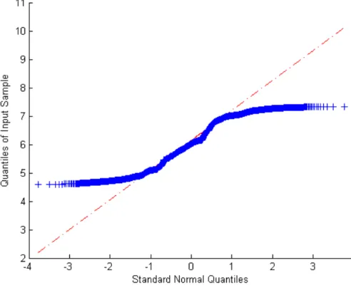
2.5 Q-Q plot of Log-prices S&P500. . . 28

3.1 Morlet’s wavelet forw0 = 5.336(real part). . . 37

3.2 Mexican hat wavelet forσ = 1 (real part). . . 37

3.3 The Cauchy wavelet for α= 3 in time representation (real part). . . . 38

3.4 Signal discontinuity. . . 41

3.5 Level-6 Multiresolution Analysis of EEG time series. . . 47

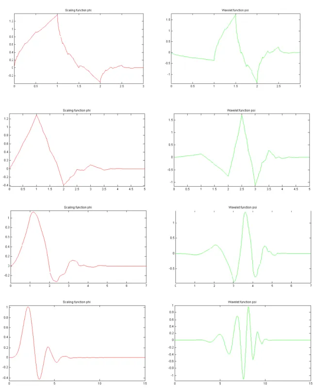
3.6 Daubechies’ scaling and wavelet functions with indices 2, 3, 4 and 8. . 51

4.1 Probability density function of α-stable distributions for different tail indices;α = 0.5; 1; 1.5; 2. . . 67

4.2 Cumulative density function of symmetric tempered stable distribu-tions for different tail indices. . . 72

4.3 Sample paths of a TS(1.2,0.5,0.5), TS(1.5,0.5,0.5) and Brownian mo-tion (solid line) . . . 79

4.4 Sample paths of a stable TS(1.7,1,0) (Dot) and a tempered stable TS(1.7,1,0.5) (solide) . . . 80

5.1 Left: soft thresholding atλ. Right: hard thresholding. . . 84

5.2 SCAD Estimator . . . 85

5.3 Denoising using mutli-level decomposition . . . 87

5.4 Denoising using mutli-level decomposition . . . 89

6.1 Sample paths of a stable TS(1.7,1,0) (Dot line) and a tempered stable TS(1.7,1,0.5) (solid line) . . . 113

6.2 Probability Density fit of the S&P 500 data. . . 116

LIST OF FIGURES 12 7.1 Wavelet Tsallis Entropy of a tempered stable process for N = 10 and

different q= 1.01; 1.5; 3; 5; 10. . . 132 7.2 Wavelet Fisher Information for tempered stable process forN = 5; 10; 15; 20.

List of Papers

The research presented in this thesis is being prepared for publication in the fol-lowing working papers:

The following paper is submitted toJournal of the Royal Statistical Society Series B. Missaoui B., McCoy E.J. Lévy Process Wavelet Prior Model.

Which has the abstract:

"In this paper, we introduce the Lévy wavelet prior model. We propose a Lévy process to capture the tail heaviness of the wavelet coefficients ubiquitous in many observed time series. We study the Besov regularity of the wavelet coefficients and establish the connection between the parameters of the Lévy wavelet prior model and Besov spaces. We gave a necessary and sufficient condition such that the realizations of the prior model fall into a certain class of Besov spaces. We prove that we can model the common phenomenon of an exponential decay across scale of the wavelet coefficients without imposing any specified structure on the variance of the wavelet coefficients. Moreover, we study a Bayesian approach under the Lévy prior model, and employ this to estimate the hyperparameters of the prior model in both a simulation study and for the S&P 500 time series."

The following paper is being prepared for submission to Entropy.

Missaoui B., McCoy E.J. The Wavelet Entropy of Tempered Stable Processes. Which has the following abstract:

"In this paper, we extend the work of Zunino et al. (2006) to non-Gaussian processes. We compute the wavelet Tsallis entropy and the wavelet Fisher’s information for

tem-LIST OF FIGURES 14 pered stable processes. Also, we introduce a regularization approach for estimating nonparametric wavelet regression. We follow here the Bayesian approach where we set the prior distribution to be tempered stable and we focus on finding a solution to the wavelet-based regression through a regularization approach based on the Tsallis entropy functional."

Chapter 1

Introduction

In recent years, nonparametric regression has gained popularity as a method of estimating real functions and Bayesian techniques have been successfully proposed to capture the statistical properties of real functions in a univariate or multivariate framework.

Many nonparametric regression estimators have been proposed. The most popular of which include smoothing splines and kernel estimators (Green and Silverman, 1994). The models are of the form

yi =g(ti) +εi, i= 1, .., n, (1.1)

with various assumptions on εi and ti. Nevertheless, these estimators may not be

satisfactory if, for example, the underlying is characterized by singularities. There-fore, wavelet-based estimators have been introduced to recover the edge structure of signals. The approach consists of expanding the data as a wavelet series and ex-tracting the wavelet coefficients. Donoho and Johnstone (1994) and Donoho et al. (1995) demonstrate that the wavelet estimators are optimal when the signal belongs to a certain class of Besov spaces. The connection between Besov spaces and wavelet statistical models was first studied by Abramovich et al. (1998).

Since then, it has been shown that the standard thresholding approaches are out-performed by Bayesian methods; see Abramovich et al. (1998) and Baraniuk and

Chapter 1. Introduction 16 Choi (1999). Mallat (1989) used the Generalized Gaussian Distribution (GGD) to model the wavelet coefficients for images as the wavelet coefficients show a heavy tailed behavior and the variance of their marginal distribution is exponentially de-caying across scale. Achim et al. (2001) and Boubchir and Fadili (2006) model the heavy-tailed behavior using an α-stable distribution as the prior and give the form of the variances across scales which ensure an exponential decay across scales. Recently, Wolpert, Clyde and Tu (2011) considered a nonparametric regression model in which the estimation is done using the atomic decomposition of the function of interest. They propose the Lévy Adaptive Regression Kernel (LARK) model which gives a prior based on Lévy random fields to the parameters of the atomic decomposition. In Wolpert, Clyde and Tu (2011, section 4), they investigate the LARK model un-der symmetric α-stable random fields and provide conditions for the LARK model to remain in the same Sobolev space (Bs

2,2) as the generating kernels. To illustrate

their methodology, they consider only the symmetric Gamma and Cauchy processes in their inference and simulation study. While a good elicitation of the hyperparam-eters of the LARK model with the symmetric Gamma prior is achieved, this is not the case with the Cauchy prior.

We similarly consider a nonparametric regression based on a Lévy wavelet prior model, but provide necessary and sufficient conditions on the hyperparameters such that the model remains in Besov spaces (B_p,qs ) with generalp and q (this is our main Theorem 32). Our approach uses a Lévy tempered stable distribution as a prior for the wavelet coefficients, where the key ingredient is the scaling property of tempered stable distributions. We demonstrate that the scaling behaviour of the tempered stable distribution can model the desired form of the wavelet coefficients without im-posing any specified structure on the variance. It can be shown that our Lévy prior model is a special case of Wolpert, Clyde and Tu’s model. If the generation function is a wavelet and the wavelet coefficients are independently tempered stable distributed, the proposed Lévy prior model can be viewed as the LARK model.

The first motivation for using the tempered stable as a prior is that its param-eters decrease faster than those of the stable distribution and make the second and higher moments finite. The second motivation is that the tempered stable density is

characterized by correlated variables and makes the variance of the underlying decay exponentially across scale.

In the same spirit of the sparse model of Abramovich, Sapatinas and Silverman (1998), we introduce the Lévy sparse prior model within a Bayesian framework. We postulate that the prior on the discrete wavelet coefficients is defined as a mixture of a tempered stable distribution and a point mass at zero. The usual approach is to extract the significant wavelet coefficients by thresholding, where the choice of the thresholding rule is then an important step in the estimation procedure. Abramovich, Benjamini, Donoho and Johnstone (2006) use the false discovery rate (FDR) method to set the threshold for the wavelet coefficients, which is based on the principle of controlling the FDR in multiple hypothesis testing. Johnstone and Silverman (2005) explore the empirical Bayes methods for level-dependent threshold selection, where they consider a mixture of a heavy-tailed density and a mass point at zero for each wavelet coefficient and show that the empirical Bayes method is stable compared to the FDR approach. In the Lévy wavelet sparse model, we consider the universal thresholding proposed in Donoho and Johnstone (1994,1995).

Assuming a tempered stable as a priori, we give a closed form to the a posteriori Lévy measure of the wavelet coefficients by applying some Bayes rule. We use this posterior Lévy measure to estimate the tempered stable distribution.

We also present a regularization approach for estimating nonparametric regression functions. We follow here the Bayesian approach where we set the prior distribution to be tempered stable and we focus on finding a solution to the wavelet-based re-gression through a Penalized Maximum Likelihood (PML) approach or Maximum a Posteriori (MAP) estimation. Here, we explore a PML based on generalized entropy functionals, namely the discrete formulation of the Tsallis entropy.

1.1 Chapter Outline 18

1.1

Chapter Outline

We give a brief description of the contents in each chapter. Chapter 2

We study the characteristics of various datasets in order to motivate the models we propose. We consider data from the S&P 500 and show that Lévy type distribu-tions are appropriate to model the wavelet coefficients.

Chapter 3

We give a brief introduction to the wavelet analysis and Besov spaces, the theory of which is necessary in later Chapters.

Chapter 4

We introduce the Lévy process which forms the structure of the wavelet prior model. We proved the key ingredient of our results, the scaling properties of tem-pered stable distributions. In this Chapter, we aim to provide basic definitions and establish a novel approach in using the wavelet theory to approximate the Wiener-Hopf factors of a Lévy process.

Chapter 5

We introduce the Lévy wavelet prior model and study the regularity and sparsity properties of the prior model in Besov spaces. In addition to this, we state the con-nection between the hyperparameters of the model and Besov spaces.

Chapter 6

We study the tempered stable prior model within the Bayesian approach in the wavelet domain and give a closed form of the Lévy density of the wavelet coefficients. We also propose a Lévy sparse mixture which is a mixture of tempered stable distri-bution and a point mass at zero. We prove that this model yields to a thresholding rule. Furthermore, we introduce an approach to estimate the hyperparameters of the prior model within a Bayesian framework. The results of Chapters 5 and 6 have been submitted (Missaoui and McCoy, 2011).

Chapter 7

We develop the wavelet entropic regularization approach. Inspired by the work of Zunino et al. (2006), we compute the wavelet Tsallis entropy and Fisher information

for a tempered stable process and proposed a penalized likelihood method for density estimation. The results of this part are ready to be submitted (Missaoui and McCoy, 2012)

Conclusion

In this concluding Chapter, we give an overview of the results obtained from the wavelet regression in the thesis. Furthermore, we discuss potentially extensions of the work presented in this.

20

Chapter 2

Data Analysis

2.1

Introduction

In financial time series analysis, the most common assumption is that asset re-turns are assumed to be Gaussian distributed. However recent empirical research shows that financial data exhibit a fat-tailed behaviour which the Gaussian distribu-tion fails to model (Rachev, 2003). Many studies considered replacing the Gaussian distribution with fat-tailed distributions e.g. the hyperbolic distribution (Bingham and Kiesel, 2001) and Gaussian mixtures (McLachlan and Peel, 2000). But these distributions are not scale-invariant; that is, their characteristics change with differ-ent time intervals. Another possibility is the Lévy stable distributions, first studied by Mandelbrot (1963). The Lévy stable distribution has fatter tails and preserves the scaling property but does not make the second and higher moments finite. The Lévy stable process is also defined by i.i.d increments and it is not characterized by correlated stochastic variables.

To remedy to these deficiencies, we will develop in this report a model based on the tempered stable distribution. In addition of having all higher moments finite, this distribution exhibits fat tails and preserves the scaling properties.

2.2

Data Analysis

Here we consider data from the S&P 500 and show that the wavelet coefficient time series of the log-returns of the data can be described by a Lévy stable type distribution; refer to section (4.3) for more details on the Lévy stable distribution and Chapter3 for details on the wavelet transform.

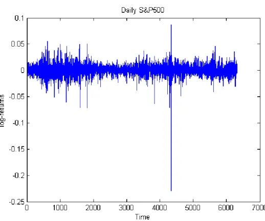
We concentrate the analysis on the daily S&P 500 ranging from January 1, 1980 to December 31, 2004 (www.yahoo.com). A plot of daily closing prices for S&P500 are given in Figure (2.3). We also present daily log-returns in Figure (2.4).

In Tables (2.1) and (2.2) we give the statistics for the log-prices and the log-returns of the daily, weekly and monthly S&P500 closing prices. It is notable that the daily log-return series show small skewness and high kurtosis which implies that the empirical distribution is almost symmetric and exhibits thicker tails than normality. The weekly and monthly log-returns time series tends to be normally distributed. That is, we will restrict our wavelet analysis to the daily log-returns.

In Table (2.3), we give the statistics of the wavelet coefficients for the daily log-returns. The coefficients were calculated using the Daubechies 3 wavelet; refer to Daubechies (1992, Chapters 6 and 7) for more details. We notice clearly that the fat-tailed behaviour of the log-returns is translated to the wavelet coefficients. The Q-Q plots in Figure (2.5) show also that the empirical distribution of the daily log-prices and the wavelet coefficients follow a non-Gaussian distribution.

The estimates of the four parameters (α, β, γ, δ) of the Lévy stable distribution are in Table (2.4), where 0 < α ≤ 2, −1 ≤ β ≤ 1, γ ≥ 0 and δ ∈ _R. We will describe the full parameterization in Chapter 4, an important parameter is α, the tail index, which gives an indication whether the times series is normally distributed (which has

α ≈ 2). A tail index α = 1.73 shows that the daily wavelet time series present fat tails. For the weekly and monthly time series, the empirical density approaches a Gaussian distribution.

The parameterγ can be interpreted as the volatility of the underlying process and we can verify from Table (2.4) thatγ is time-dependent and thus the underlying cannot be modeled with a stochastic process with i.i.d increments.

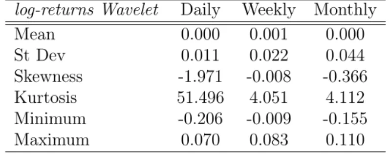
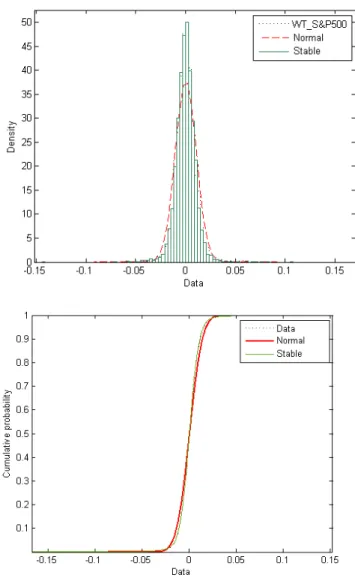
2.2 Data Analysis 22 The statistical properties of the wavelet coefficients of the daily log-returns also show that as the sampling time interval∆tincreases, the mean increases and the ratio of the mean and the standard deviation decreases. This is consistent with the characteristics of a power law. Recently, Wei and Billings (2009) have shown that foreign exchange rates obey power-laws and therefore belong to the class of selfsimilar processes. In Figures (2.1) and (2.2), we present a comparison between the Gaussian and Lévy stable densities and cumulative density functions in fitting the wavelet coefficient series. We can see that the Gaussian density is not an appropriate model and that the Lévy stable density provides a much better central and extremal fit.

We can also see that the leptokurtic behaviour of the daily log-returns and the wavelet coefficients series disappears for weekly and monthly time intervals.

We observe that the Lévy stable distribution describes the daily log-returns well at different time intervals. However with the assumption of i.i.d increments and having an infinite second moment, the Lévy stable process is not an appropriate model for an underlying having scaling properties.

An alternative is to model the empirical distribution with a truncated Lévy flight (TLF) distribution. The probability distribution of a TLF process is defined by:

f(x) =            0, if l > 0, L(x), if −l < x < l, 0, if x <−l. where L(x) = 1 π Z +∞ 0 exp(−γwα) cos(wx)dw

is the symmetric Lévy stable distribution with tail indexαandγ the scale parameter. The parameter l is the cutoff length.

The TLF distribution has a finite second moment and thicker tails. Mantegna and Stanley (1995) showed that the scaling property of the TLF distribution is preserved for small time intervals and the TLF tends to the Gaussian distribution as the time interval increases. However, the TLF is not an infinitely divisible distribution and

therefore it does not correspond in a natural way to a Lévy process; see Chapter 4 for background on Lévy processes.

What we need is a model with the same characteristic of the Lévy stable distribution but with finite second- and higher-order moments. That is, a model which behaves in a short time like a stable process and in long time tends to Brownian motion; see section 4.6. Such a model is the tempered stable distribution, which we will introduced in section 4.5.

2.3

Conclusion

In this chapter we introduced the data sets which form the motivation for our study. We have discussed the log-prices and the log-returns of the S&P500. We also investigated the characterization of the wavelet coefficients time series.

In the next chapter we introduce the basics of wavelet analysis that we need in the development of our framework.

2.3 Conclusion 24 Table 2.1: Descriptive Statistics of log-prices for S&P500

log-price Daily Weekly Monthly

Mean 6.045 6.046 6.050

St Dev 0.801 0.802 0.801 Skewness -0.053 -0.054 -0.061 Kurtosis -1.242 -1.243 -1.244 Minimum 4.587 4.611 4.626

Table 2.2: Descriptive Statistics of log-returns for S&P500 log-returns Daily Weekly Monthly

Mean 0.000 0.002 0.008 St Dev 0.011 0.022 0.045 Skewness -1.743 -0.495 -0.895 Kurtosis 38.822 3.043 3.551 Minimum -0.229 -0.130 -0.245 Maximum 0.087 0.085 0.124

Table 2.3: Descriptive Statistics of Wavelet Coefficients of log-returns for S&P500 log-returns Wavelet Daily Weekly Monthly

Mean 0.000 0.001 0.000 St Dev 0.011 0.022 0.044 Skewness -1.971 -0.008 -0.366 Kurtosis 51.496 4.051 4.112 Minimum -0.206 -0.009 -0.155 Maximum 0.070 0.083 0.110

Table 2.4: Parameter estimates of the log-Stable for the wavelet coefficients of the log-returns for S&P500

log-Stable Wavelet α β γ δ

Daily 1.7365 0.0643 0.0058 0.0011

Weekly 1.8654 0.0581 0.0144 0.0011 Monthly 1.8822 -0.7439 0.0292 0.0040

Figure 2.1: Empirical PDF and CDF Fitting of the wavelets coefficients of the daily log-returns S&P500

2.3 Conclusion 26

Figure 2.2: Left and right tails of the CDF of the wavelets coefficients of the daily log-returns S&P500

Figure 2.3: Daily Log-prices S&P500

2.3 Conclusion 28

Chapter 3

Wavelet Analysis

3.1

Introduction

Until 1970, the predominant assumption was that signals were appropriately mod-eled as realizations of Gaussian processes, in consequence under the assumption of stationarity, linear algorithms based on the Fourier transform were considered op-timal. The situation has been revolutionized with the development of novel image processing techniques in the 1980’s. Images are poorly modeled by Gaussian pro-cesses, and the edge components of image such as contours are often more important. The use of nonlinear algorithms became necessary, which opened signal processing to modern mathematics and wavelet analysis. The inadequacy of the Fourier transform to describe non-stationary behavior of a function will be the basis of the motivation to introduce this concept.

3.2

Fourier Transform

For simplicity, we will introduce the Fourier analysis in one-dimension; refer to Papoulis (1987) and Dym and McKean (1972) for more details. We recall that a Hilbert space is a space which has an inner producthx, yiand which is complete with respect to the norm ||x||=hx, xi1/2. We also recall that a spaceE is called complete

3.2 Fourier Transform 30 if every Cauchy sequence in E converges in E. We denote L2(_R) the collection of all complex-valued Lebesgue-measurable functions in _R such that R

R|f(t)| 2_{dt < ∞.} That is, L2(_R) = f :_R→_C| Z R |f(t)|2dt <∞ . L2(_R) is a Hilbert space with the inner product

hf, gi=

Z

R

f(t)g(t)dt,

and the norm ||f||= R

R|f(t)|

2_dt1/2 _{<∞, where g means the complex conjugate of} g.

Definition 1. Assume that f ∈ L2₍

R), the Fourier transform of f is the function

Ff defined by

Ff(w) =

Z

R

e−itwf(t)dt. (3.1)

We usually write fˆfor Ff and it is a function of a parameter w which we call the angular frequency. Assuming fˆ∈ L2₍

R), the following proposition gives the inverse

Fourier transform. Proposition 2. If fˆ∈L2₍ R) and f ∈L2(R), then f(t) = 1 2π Z R eitwfˆ(w)dw. (3.2)

The Fourier transform preserves the inner scalar product (Parseval formula):

Z R f(t)¯g(t)dt = 1 2π Z R ˆ f(w)¯gˆ(w)dw.

Forf =g, we obtain the energy conservation known as the Plancherel formula:

Z R |f(t)|2dt= 1 2π Z R |fˆ(w)|2dw.

We write f ∗g for the convolution f∗g(x) =R

Proposition 3. If f, g∈L2(_R), then almost everywhere

[

f∗g(w) = ˆf(w)ˆg(w).

Given a function f we define the translation operator Tb by Tbf(x) = f(x−b) for

b ∈_Rand the dilation operator Da byDaf(x) =|a|−1/2f(x−a) for a∈R-{0}. It is

easy to prove that

FTbf(w) = e−ibwfˆ(w),

FDaf(w) = |a|1/2fˆ(aw).

3.2.1

Fourier Transform and Regularity

The Fourier transform provides a way to characterize the overall regularity as well as the related concept of the frequency scale of a function. Roughly speaking, the regularity measures the smoothness of a function while the frequency scale measures how quickly the function oscillates; a natural way to describe the global regularity of a function and capture its frequency scale is to consider functional Sobolev spaces (see e.g Adams (1978)).

The Sobolev space Hm₍

R) is defined to be the set of all functions f ∈ L2(R) such

that for every α with |α| ≤m, the partial derivative ∂α_{f ∈L}2₍

R), that is

Hm(_R) =f ∈L2(_R)|∂αf ∈L2(_R), α∈_R .

Hm(_R)is a Banach space equipped with the norm ||f||Hm =

X

|α|≤m

||∂αf||L2₍

R).

Sometimes the properties of regularity of a function cannot be seen directly from the above definition of the Sobolev spaces. Therefore, it has been shown that it is interesting to investigate the regularity by means of the Fourier transform. The

3.2 Fourier Transform 32 Sobolev space Hm(_R) can be equivalently defined by

Hm(_R) = f ∈L2(_R)| Z R (1 +|w|2₎α_|fˆ(w)|2_{dw <+∞, α∈} R .

The Fourier transform allows us to study the global regularity and to determine which Sobolev space the function belongs to. However, it does not describe and analyze the local regularity since a function can be locally regular without being globally regular; e.g., the Heaviside function is constant over_R-{0}but does not belong to any Sobolev space with positive index.

Moreover, many signals in reality, such as speech, music and images, have changing frequency characteristics, i.e. frequencies vary with time, and the Fourier transform does not contain information on the time evolution of the frequencies. To achieve a time-dependent frequency analysis, we introduce the Gabor transform characterized by the short-time Fourier transform.

3.2.2

Short-Time Fourier Transform

To convey simultaneous time and frequency localization in a signal, Gabor (1940) introduced the short-time Fourier transform (STFT). In practice, this Gabor trans-form consists in multiplying the function by a window function h which is nonzero for only a short period of time. For u, w ∈_R, the STFT for a function f ∈L2₍

R) is defined by T S(u, w) = Z R f(x)h(x−u)e−iwxdx.

Putting u = na and w = mb where n, m ∈ _Z and a, b ∈ _R, we can compute the Fourier coefficients of the product

dmn(f) =

Z

R

f(x)h(x−na)e−imbxdx.

The coefficients dmn represent in this formulation the intensity of the frequency mb

written using the Fourier series expansion

f(x) =X

n,m

dmn(f)h(x−na)eimbx.

We will assume in the Gabor representation that the window function h satisfies

A≤

N

X

n=1

|h(x−na)|2 _≤B,

for A, B ≥0. The Gabor transform is numerically stable whenB is not too large. Morlet suggested to compute the inner product of f with an analyzing function

1 √ a0ψ x−x0 a0

which we expect to be localized in frequency and in time. The function

ψ is calledwavelet.

If we denote byxψ andνψ the mean values ofxand ν with respect to the probability

measure|ψ(x)|2_{dx and |ψˆ(ν)|}2_{dν, then we can write}

xψ = Z +∞ −∞ x|ψ(x)|2_dx, νψ = Z +∞ −∞ ν|ψˆ(ν)|2_dν.

We can also write the resolution of the analyzing waveletψ in terms of spreads around

xψ and νψ. The spreads are measured by the variance and defined by

∆x2_ψ = Z +∞ −∞ |x−xψ|2|ψ(x)|2dx, ∆ν_ψ2 = Z +∞ −∞ |ν−νψ|2|ψˆ(ν)|2dν.

The joint time-frequency resolution is defined by the product of the two resolutions ∆xψ∆νψ. This joint resolution depends on a0. This represents in itself a downfall

of the Gabor transform and the wavelet analyzing function; that is, it is impossible to find a0 which gives at the same time good frequency and good time resolution.

This means that a window function h or a wavelet ψ with finite energy compactly supported in time and frequency does not exist. This is justified by the Heisenberg

3.3 Wavelet Transform 34 uncertainty principle, which states

Theorem 4. Let ψ ∈L2(_R) and for any νψ, xψ ∈R, we have

∆xψ∆νψ ≥

1 2,

and the minimum value 1₂ is reached for Gaussian functions.

3.3

Wavelet Transform

One of the reasons for the creation of the wavelet transform is to define a window function that is well-localized in time and frequency. The purpose of this section is to give a short introduction to wavelets. For more extensive treatments, see, for example, Mallat (1999), Meyer (1992) and Walden and Percival (2001). The term wavelets is used to refer to a dictionary of basis functions. The wavelet structure may be considered as a generation of an orthonormal wavelet basis for functionsg ∈L2(_R).

3.4

Continuous Wavelet Transform

A wavelet ψ is a real function inL2₍

R) satisfying theadmissibility condition

Cψ =

Z +∞

0

|ψb(w)|2

w dw <∞, (3.3)

where ψbis the Fourier transform of ψ and the integral of ψ has to vanish Z

ψ(x)dx= 0. (3.4)

Also, the square of the wavelet should integrate to unity,

Z ∞

−∞

ψ2(x)dx= 1.

The integral (3.4) is the value of the Fourier transform of ψ at 0. Setting ψb(0) = 0,

One way of selecting a wavelet function is given in the following theorem. Theorem 5. Let φ and φ(n) _{be L}2₍

R) functions for n > 0. Let φ(n)(x) 6= 0 and

satisfies (3.4). Then, ψ(x) =φ(n)_{(x) is a wavelet function.}

Proof. We need to prove that Cψ <∞.

Cψ = Z +∞ 0 |ψb(w)|2 w dw = Z |w|≤1 |w|2n−1_|φˆ(w)|2_dw+ Z |w|>1 |w|2n_|φˆ(w)|2 |w| dw ≤ Z |w|≤1 |φˆ(w)|2_dw+ Z |w|>1 |wnφˆ(w)|2_dw Finally, Cψ ≤ kφk 2 2+ φ(n) 2 2 <∞.

The regularity of a wavelet is characterized by its moments. A wavelet hasmvanishing moments if

Z +∞

−∞

xpψ(x)dx= 0, for p= 0, ..., m−1.

The wavelet function is then obtained by dilation and translation of ψ:

ψt,s(x) = TtDsψ(x) = 1 √ sψ x−t s .

The continuous wavelet transform W f of a function f ∈L2(_R) is defined by

W f(t, s) = Z ∞ −∞ f(x)√1 sψ x−t s dx=f∗ψs(t), whereψs(t) = √1_sψ −t_s

. Using the Pancherel formula, we might compute the wavelet coefficients in Fourier space via

W f(t, s) =√s Z ∞

−∞

ˆ

f(w)ψ¯ˆ(sw)eiwtdw. (3.5)

Like the Fourier transform, the wavelet transform has an inversion formula which allows us to reconstruct the function from its wavelet transform.

3.4 Continuous Wavelet Transform 36 Theorem 6. Let ψ ∈ L2(_R) be an analysing wavelet, then for any f ∈ L2(_R), we have f(t) = 1 Cψ Z +∞ 0 ds s2 Z +∞ −∞ W f(x, s)ψt,s(x)dx. (3.6)

Proof. Using (3.5), we can write the right hand side of (3.6) as

g(t) = Z +∞ 0 Z +∞ −∞ W f(x, s)√1 sψ t−x s dxds s2, = Z +∞ 0 ds s Z +∞ −∞ dx Z +∞ 0 dwfˆ(w)ψ¯ˆ(sw)eiwt1 sψ t−x s , = Z +∞ 0 Z +∞ 0 ˆ f(w)ψ¯ˆ(sw) ˆψ(sw)eiwtdxds s , = Z +∞ 0 dwfˆ(w)eiwt Z +∞ 0 ds s | ˆ ψ(sw)|2, = Cψf(t),

where we used the inverse formula for the Fourier transform of f. Also, we have the Pancherel formula in the form

||f||2_L2(R)= 1 Cψ Z +∞ 0 Z +∞ −∞ |W f(x, s)|2dxds s2. (3.7)

Here, we will give some examples of analyzing wavelet functions. Example 1 (Morlet’s Wavelet)

The Morlet wavelet was used first in seismic signals and geophysical explorations. It is complex-valued and obtained by shifting the Gaussian function in the Fourier domain:

ψ(t) = eiw0t_e−t2/2_,

where w0 is a constant. This wavelet is not admissible, since it is not of zero mean.

Its Fourier transform does not vanishes at the origin: ψˆ(0) = √2πe−w20/2. However, for large values of w0, the value of ψˆ(0) is small and therefore the Morlet wavelet

with w0 = 5.336.

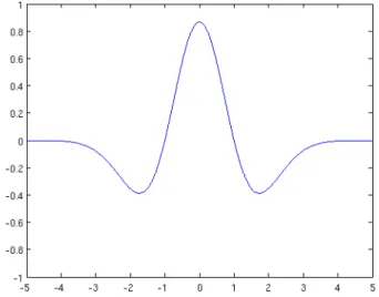
Example 2 (Mexican hats)

The Mexican hats are defined as the second derivative of the Gaussian function (see Figure (3.2)). The normalized Mexican hat wavelet is

ψ(t) = 2 π1/4√_3σ t2 σ2 −1 e−t2/(2σ2).

Figure 3.1: Morlet’s wavelet for w0 = 5.336(real part).

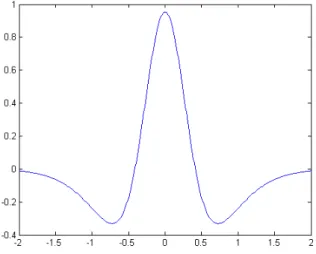
3.4 Continuous Wavelet Transform 38 Example 3 (Cauchy wavelets)

The Cauchy wavelets are analytic functions and their general expression is (Figure 3.3)

ψ(t) = 1 2π

Γ(α+ 1)

(1−it)1+α, α >0, (3.8)

where Γ(t) =R₀∞tz−1_e−t_{dt. The Fourier transform of Cauchy wavelet is}

b ψ(w) =    wα_e−w _{if w >0,} 0 otherwise.

Therefore, the Cauchy wavelet transform is closely related to the analysis of the analytic functions over half-plane; refer to section 3.4.2 for more details. In section 4.7, we present an application of Cauchy wavelets to compute the Wiener-Hopf factors.

Figure 3.3: The Cauchy wavelet for α= 3 in time representation (real part).

3.4.1

Regularity

One of the most important properties of wavelets is their high accuracy at fine scales. This feature is intrinsically embedded in their construction. Therefore, it is natural that wavelets may be used to characterize regularity properties of singular structures, and the decay of the wavelet coefficients across scales is related to the

Lipschitz (global) or pointwise Lipschitz (local) regularity. Let0< α <1. We introduce the α-Lipschitz space:

Lα ={f :_R→_C, ∃K <∞:|f(x)−f(y)| ≤K|x−y|α, ∀x, y ∈_R}.

The conventional way to characterize α-Lipschitz functions is based on the Fourier transform. We can show that iff is bounded and satisfies

Z

R

|fˆ(w)|(1 +|w|α_{)dw <∞, (3.9)}

then f ∈Lα_{. The converse is in general false (see e.g Adams (1978)).}

For wavelet analysis, we will see that the results are similar. The following result follows the same philosophy as the analogue for Fourier transform of Lipschitz func-tions:

Theorem 7. Let f ∈ L1(_R) be α-Lipschitz over [a, b] and ψ an analyzing wavelet such that ψ ∈L1₍

R) and xαψ ∈L2(R). Then there exists C > 0 such that

∀(t, s)∈[a, b]×_R+ , |W f(t, s)| ≤Csα+1/2. (3.10)

Conversely, if f is bounded and W f(t, s) satisfies (3.10), then f is α-Lipschitz on [a+, b−] for any >0.

The inequality (3.10) is a similar to the Fourier condition (3.9) wheres plays the role of the inverse of the frequency. It gives an asymptotic behaviour of the decay of the wavelet transform when s goes to zero.

The continuous wavelet transform can also characterize the regularity off at a point

t0. Jaffard (1991) gave necessary and sufficient conditions on the wavelet transform

for estimating theα-Lipschitz of f att0. We consider a compactly supported wavelet ψ havingn vanishing moments.

Theorem 8. Letf ∈L2₍

3.4 Continuous Wavelet Transform 40 such that ∀(t, s)∈[a, b]×_R∗+ _{, |W f(t, s)| ≤As}α+1/2 1 + t−t0 s α . (3.11)

Conversely, if α < nand α is not an integer, and there existsAand α0 < αsuch that

∀(t, s)∈[a, b]×_R∗+ , |W f(t, s)| ≤Asα+1/2 1 + t−t0 s α0! . (3.12) then f is α-Lipschitz at t0.

We refer to Mallat (1998) and Jaffard (1991) for the proof of the results (3.10), (3.11) and (3.12).

This analysis was refined by Jaffard (1991), who has shown that wavelet analysis can be viewed as a simple version of a larger program, namely two-microlocalization theory introduced by Bony (1981) to study the solution of hyperbolic partial differential equations. We refer to Jaffard and Meyer (1993) for a background and references. Figure (3.4) shows the discontinuity response of a locally perturbed signal in the first level detail coefficients and the wavelet coefficient at the discontinuity point.

3.4.2

Hardy Spaces

In this section, we give the basic definitions and results of Hardy spaces that we need in our development in section 4.7. Our aim will be to use Hardy spaces to approximate the Wiener-Hopf factors of a Lévy process. For a complete and rigorous exposition of Hardy spaces, see Duren (1970) or Koosis (1980).

Definition 9. We say that an analytic function f belongs to H₊2(_R) if

sup y>0 Z |f(x+iy)|2_dx 1/2 <∞.

The analogue holds for H2

−(R) but the supremum is on the lower-half plane (y <0).

Figure 3.4: Signal discontinuity. Definition 10.

H₊2(_R) = {f ∈L2(_R)| supp( ˆf)⊂[0,+∞)}, H₋2(_R) = {f ∈L2(_R)| supp( ˆf)⊂(−∞,0]}.

The two definitions of Hardy spaces given in Defintions 9 and 10 are similar; their equivalence follows easily from the Parseval formula.

H₊2(_R)(resp. H−2(R)) is a closed subspace ofL2(R)with functions having only positive

(resp. negative) frequencies. They can be identified with H2

±(R) = F±(L2(R)); see

Ruth and Van Fleet (2009).

Using the Plancherel formula, the standard perpendicular decomposition

L2(_R) =L2(_R−)⊕L2(R+).

becomes the non-trivial decomposition

3.5 Multiresolution Analysis 42 The functions that belong to H₊2(_R) (resp. H₋2(_R)) are called progressive (resp. regressive). Also, the orthogonal projectors P± : L2₍

R) → H±2(R) are expressed in

terms of the Hilbert transfrom as follows:

P± = 1

2(1±iH), (3.14)

where Hfˆ (w) = −i sgn(w)f(w) is the representation of the Hilbert transform in Fourier space. We recall here that the Hilbert transform is

Hf(t) = 1 πlim→0 Z |t−x|> f(t) t−xdt.

As an example, the Cauchy wavelet defined in (3.8) is progressive. Its Fourier trans-form is ˆg(w) = wα_e−w₁

{w>0}. That means, its Fourier coefficients for negative

fre-quencies are zero.

The decomposition (3.13) gives an easy way of decomposing the analyzed function and the analyzing wavelet into a sum of functions belonging to H2

+(R) and H−2(R).

Letg ∈L2₍

R). Using Theorem 6, we have

g(x) = Z +∞ 0 da a2 Z +∞ −∞ ψa,b(x)W g(a, b)db,

where ψa,b(x) = a−1/2ψ(x_a−b)with a >0 and W g(a, b) = hg, ψa,bi.

The perpendicular splitting (3.13) provides us with a way of decomposing g into

g =g1+g2. It is enough to split the wavelet coefficients of g into a sum of W g+ and W g−, where W g+ ∈H+2(R) and W g− ∈H−2(R), and then reconstruct g1 = T(W g+)

and g2 =T(W g−) whereT is the reconstruction wavelet operator which takesW g to

g.

3.5

Multiresolution Analysis

Mallat (1999) and Meyer (1992) introduced the concept of multiresolution anal-ysis (MRA) as a tool to construct a wavelet orthonormal basis. This notion comes

within the framework of multiscale approaches for which the work of Haar, Franklin and Littlewood-Paley are the precursors. In this section, we will introduce Mallat’s representation of the MRA, which states that wavelets can be designed from discrete filters. For more details, see Mallat (1999).

3.5.1

Theoretical framework

Definition 11. A multiresolution analysis is a sequence of subspaces ofL2(R)denoted

by (Vj)j∈_Z, which has the following properties:

Vj ⊂ Vj+1, \ j∈_Z Vj = 0, [ j∈Z Vj = L2(R), f(t)∈V0 ⇐⇒ f(2jt)∈Vj,

and there exists a function φ(t)∈V0 such that (φ(· −k))k∈_Z is an orthonormal basis

for V0.

Roughly speaking, multiresolution analysis decomposes L2(R) into nested

se-quences of (Vj)j∈Z named the approximation spaces. The space Vj provides a

bet-ter approximation to a function f in L2(R) as j tends to infinity. The spaces Wj ⊂ Wj+1 such that Wj is a subset of Vj+1 are called detail spaces. If we

ap-proximate fj+1(t)∈Vj+1 by fj(t)∈Vj, then gj(t)∈ Wj holds the details we need to

add to fj(t) to recoverfj+1(t) =fj(t) +gj(t).

In the sequel, we will often write φn(t) = φ(t − n). For H a Hilbert space and

(φn)n∈Z∈H, if there exist two constants 0< A < B such that

AX n∈_Z c2_n ≤ X n∈_Z cnφn(t) 2 ≤BX n∈_Z c2_n,

for any sequence(cn)n∈Z, then the sequence (φn)n∈Z is a Riesz basis ofH (Daubechies

3.5 Multiresolution Analysis 44 Theorem 12. For {Vj}j∈Z a multiresolution analysis for L2(R), there is a unique

function φ∈L2(R) such that

{φjk :x→2j/2φ(2jx−k)}k∈Z,

forms an orthonormal basis of the space Vj.

Since φ belongs to V0 and V0 belongs to V1, we can write φ as a linear combination

of {φ1,k}k∈Z. This means that there exists a square integrable sequence{hk}k∈Z such

that

φ(t) =√2X

k∈Z

hkφ(2t−k), (3.15)

and the Fourier transform of φˆof φ satisfies ˆ φ(w) =m0 w 2 ˆ φw 2 , (3.16) wherem0(w) = √1₂P_k∈Nhke

−ikw_{. It is straightforward to see thatm}

0 is a2π-periodic

function. The function m0 is called the scaling filter. One remarkable and useful

property is that the orthonormality of the (φn)n∈Z can be restated in terms of φˆand

m0.

Theorem 13. Assume φ ∈ L2₍

R). The set (φn)n∈Z forms an orthonormal basis if

and only if X k∈Z ˆ φ(w+ 2πk) 2 = 1. (3.17)

Moreover, if φ generates a multiresolution analysis (Vj)j∈Z, then

|m0(w)| 2

+|m0(w+π)| 2

= 1. (3.18)

Proof. See Ruch and Van Fleet (2009) Theorem 5.5.

The multiresolution approximation at resolution j of a function f ∈L2(R) is

of f on Vj. These projections will construct Riesz bases of wavelets in the Hilbert

space L2(R).

If f ∈ L2(R), the difference PV j+1f −PV jf between resolutions j and j + 1 is the

orthogonal projection off onWj, the orthogonal complement ofVj inVj+1. We write

Vj⊕Wj =Vj+1, (3.19)

and

PVjf+PWjf =PVj+1f. (3.20) The complement PWjf provides the details that appear at scale j+ 1.

Hence, we construct a function ψ such that {x 7→ ψ(x−k)}k∈Z is an orthonormal

basis of W0. The function ψ is the wavelet and for any j ∈ Z the set {ψjk : x →

2j/2_ψ(2j_x−k)}

k∈_Z forms an orthonormal basis of Wj. Moreover, as W0 belongs to V1, there exists a sequence of real variables {gk}k∈Z such that

ψ(t) =√2X

k∈Z

gkψ(2t−k). (3.21)

This defines the second wavelet filterm1 such asψˆ(w) =m1(w/2) ˆψ(w/2)and defined

by m1(w) = 1 √ 2 X k∈z gke−ikw.

By mimickingm0, the function m1 also satisfies

|m1(w)|2+|m1(w+π)|2 = 1, m0(w)m1(w) +m0(w+π)m1(w+π) = 0.

In practice, we normally choose m1 to be expressed in terms of m0 and we have m1(w) = −e−iwm0(w+π).

Moreover, by iterating the equation (3.19), we obtain

Vj⊕Wj⊕...⊕W_j0

−1 =Wj0, if j < j

0

3.5 Multiresolution Analysis 46 If j0 →+∞ (and resp. also j → −∞), we obtain two decompositions:

L2(R) = Vj ⊕ +∞ M j0=j W_j0, for all j ∈_Z, L2(R) = +∞ M j0=−∞ W_j0.

The union of all Riesz bases in each of these direct sums provides several wavelet bases

Bj = {φjk :k∈Z} ∪ {ψj0k :j

0

≥j, k ∈_Z},

B = {ψjk :j ∈Z, k∈Z}.

Using equation (3.19), we can write

V0 = V−1 +W−1

= V−2 +W−2+W−1

= V−J +W−J +...+W−1,

This leads to the decomposition of a signal x(t)

x(t) = A1(t) +D1(t)

= A2(t) +D2(t) +D1(t)

= AJ(t) +DJ(t) +...+D1(t),

whereDi(t)∈W−i is called the detail at leveli, andAi(t)∈V−i is called the

approx-imation at level i.

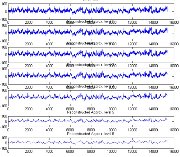
Figure (3.5) shows a multilevel wavelet denoising of the EEG time series. We use Mat-lab functionwavedecto perform a multilevel analysis to six levels with Daubechies-3 wavelets; refer to section 3.6 for background on Daubechies wavelet. Then we re-construct the approximations at various levels using the Matlab function wrcoef. A

significant denoising occurs with level-6 approximation coefficients. The data corre-sponds to the recording on a different subject in the left occipital electrode (O1), with linked earlobes reference (http://www.vis.caltech.edu/ rodri/data.htm).

Figure 3.5: Level-6 Multiresolution Analysis of EEG time series.

3.6

Discrete Wavelet Transform

Like the Fourier transform, the wavelet transform has a discrete and a continuous version. Following the approach of Daubechies (1992), wavelet series are generated

3.6 Discrete Wavelet Transform 48 by dilations and translations of a function ψ, called the mother wavelet:

ψjk(t) = 2j/2ψ(2jt−k), j, k∈Z,

The set of {ψjk|j, k ∈ Z} forms an orthonormal basis in L2(R). Given the wavelet

basis, the wavelet series representation of a function g ∈L2₍

R)is then

g(t) = X

j,k∈Z

djkψjk(t),

where the wavelet coefficients djk are given by

djk =

Z

R

g(t)ψjk(t)dt.

The Discrete Wavelet Transform (DWT) can be computed with a convolution of discrete filters. Mallat (1987) suggested a method of constructing wavelet orthogonal bases using the Fast Fourier Transform (FFT).

Let the sequences {hk}k∈Z and {gk}k∈Z defined in (3.15) and (3.21) be a pair of

response filters. We construct a scaling function φ and the corresponding wavelet function ψ inL2(R) such that

b φ(w) = +∞ Y k=1 m0 w 2k , b ψ(w) = m1 w 2 b φw 2 .

These equations show that the infinite product converge uniformly on compact sets, and that φ has a compact support; see Daubechies (1999) Chapter 7. Using discrete filters reduces the complexity of the wavelet design. Instead of constructing an ap-propriate scaling function and the corresponding wavelet function, we simply choose the discrete set of coefficients of the filters.

Daubechies’ idea was to construct a compactly supported orthonormal wavelet basis with compact support depending on an integerN which defines the support and the degree of regularity, namely Daubechies wavelet DAUBN. The goal was then to find

a trigonometric polynomial m0 satisfying m0(0) = 1and |m0(w)| 2 +|m0(w+π)| 2 = 1, and QN j=1m0( w 2j)1[−π,π](₂wN) converges to Q∞ j=1m0( w 2j) inL2. Daubechies studied this problem in terms of |m0(w)|

2

instead ofm0 and proved that

the trigonometric polynomial of the following form is a good choice:

m1(w) =|m0(w)|2 = N−1 X k=0 2N−1 k 1 + cosw 2 2N−1−k 1−cosw 2 k (3.22)

Daubechies’ fundamental result was that the choice of the polynomial |m0(w)| 2

with degree 2N −1 led to a compactly supported orthonormal scaling function φN with

support on [0,2N −1] and degree of regularity αN ∼ (1− _{2 log 2}log 3 )N when N → ∞.

Moreover, since m1(w) has a root w = π of multiplicity N, m1(w) can be written

in terms of the Strang and Fix condition which states that any polynomial of degree ≤N −1can be written of the form P(x) = P

k∈ZhP|φN(x−k)iφN(x−k).

For example, When N = 1, we obtain DAUB2 Daubechies and we find |m0(w)|2 =

1 + cosw

2 .

The correct choice for m0 would be m0(w) = 1+e₂−iw. Therefore, we can calculate the scaling functionφ b φ(w) = lim N→∞ N Y j=1 1 2 1 + exp −iw 2j .

We can verify that φb(w) = 1−e

−iw

iw which implies that φ(x) = 1x∈{[0,1]}.

LetαH be the supremum ofβ such that

Z

(1 +|w|β)|φˆ(w)|dw <∞.

3.7 Besov spaces 50 is defined by (Vidakovic, 1999 p.37) 1. 0< s <1, _Cs₍ R) = n f ∈L∞(R) : sup|f(x+|hh)|−sf(x)| <∞ o , 2. s=n+s0, 0< s0 <1, _Cs₍ R) = f ∈L∞(R)∩Cn(R) : d n dxnf ∈Cs 0 (_R) . N 1 2 3 4 5 6 7 8 9 10 αH 0.550 0.915 1.275 1.596 1.888 2.158 2.415 2.661 2.902

Table 3.1: Hölder regulatity of Daubechies scaling functions (Table 3.3, Vidakovic (1999))

From Table 3.1, we can see thatDAUB4 is the first differentiable wavelet with Hölder coefficient αH = 1.275 >1. Figure (3.6) shows the plots of Daubechies’ wavelets for

different indices 2,3, 4 and 8.

3.7

Besov spaces

Like Sobolev spaces, it has also been shown that in Besov spaces the smoothness of functions can be expressed in terms of approximation schemes and described through derivatives and differences; refer to Triebel (1992).

In this section, we introduce some relevant aspects of Besov spaces. Of especial importance is the connection between the wavelet theory and the Besov spaces. This connection is the key ingredient of the study of the smoothness of the prior model. The relationship between the hyperparameters of the prior model and the parameters of Besov spaces has been already investigated in Abramovich et al. (1998). For more details on functional spaces, refer to Triebel (1983).

We consider the family of Besov spaces Bs

p,q(I), I = [0,1], 0< s < ∞, 0 < p≤ ∞,

and 0 < q ≤ ∞. These spaces have, roughly speaking, s derivatives in Lp(I); The

third parameterqallows one to make finer distinctions in smoothness. For p=q = 2,

Bs

p,q(I) is the Sobolev spaces Hs(I).

For p < 1 or q < 1, these spaces are not Banach spaces, but rather quasi-normed linear spaces. This means that the triangular inequality may not hold and it

3.7 Besov spaces 52 is replaced by the inequality

||f+g||Bs

p,q(I) ≤C(||f||Bsp,q(I)+||g||Bp,qs (I)). (3.23) where C is a constant, f and g in Bs

p,q(I). We recall here that a quasi-normed space

is a quasi-Banach space if it is complete with respect to the quasi-norm in question. For simplicity, we shall continue to call these quasi-norms norms. We also wish to characterize Besov spacesBs

p,q in terms of means of differences.

For any h ∈ _R, we define ∆0

hf =f(x) and let for x ∈ I, the mixed differences ∆khf

adapted to I of order k and step h is defined by

∆k_hf(x) = k X j=0 (−1)k−j k j f(x+hj), k∈_N, h∈_R. (3.24) We recall that ∆k

h can also be defined by

∆k_h+1f(x) = ∆k_hf(x+h)−∆k_hf(x), k= 0,1, ... (3.25) We define theLp(R)-mixed modulus of continuity or means of differences, 0< p≤ ∞

as wr(f, t)p = sup|h|≤t Z Irh |∆k_hf(x)|p_dx 1/p , (3.26)

with the usual change to an essential supremum when p = ∞. Given s > 0, 0 < p ≤ ∞, and 0 < q ≤ ∞, choose r ∈ _Z with r−1 ≤ s ≤ r. Then the Besov space seminorm is defined as |f|Bs p,q(I) = Z ∞ 0 (t−swr(f, t)p)q dt t 1/q , (3.27)

again with a supremum when q=∞. The Besov space is defined by

B_p,qs ={f ∈Lp(I), ||f||Bs

where

||f||Bs

p,q(I) =|f|Bp,qs (I)+||f||Lp(I), (3.29) and Lp(I)is the class of functionsf with ||f||p = (

R

I|f(x)|

p_dx)1/p _{<∞ if0< p <∞}

and ||f||∞= inf(m:|f(x)| ≤m) if p=∞. Since the Besov spaces can be

character-ized via moduli smoothness onI and admit wavelet decompositions, we can define a Besov sequence norm on the wavelet coefficients.

In the following we give the definition of the Besov norm as a function of the wavelet coefficients of a function which belongs to the Besov space.

To provide a better understanding of what is going on we will introduce the Littlewood-Paley decomposition. Calderón in 1960 introduced a well-known decomposition of the identity operator. Let ψ ∈ L2(_R) such as ψˆ ∈ C∞_{, and compactly supported with}

Supp( ˆψ) 6= 0. We define the convolution operator Qt as Qtf = f ∗ ψt(x) where

ψt(x) = 1_tψ x_t

. The Calderón formula is written as

Z +∞

0

Qt◦Q∗t

dt

t =CψI, (3.30)

where Q∗_t is adjoint operator. If we define ∆j =Q1/2j ◦Q∗

1/2j, then the Calderón formula (3.30) is replaced by the Littlewood-Paley decomposition

f =X

j∈Z

∆jf.

Therefore, the characterization of Besov space in terms of Littlewood-Paley is

B_p,qs =    f ∈ S0 | ∞ X j=0 2jsq||∆jf||q_Lp₍ R) !1/q <∞    ,

where S0 _{is the set of all tempered distributions on} R.

For f ∈B_p,qs , suppose thatf has a wavelet series expansion f(x) = P

j,k∈Zdjkψjk(t)

such that P_|ˆ

ψ2₍₂−j_{ξ)|= 1 almost everywhere for ξ∈}

3.8 Summary 54 Armed with Littlewood-Paley decomposition, the Besov sequence norm for f is de-fined by ||f||Bs p,q = |d00|+      ∞ X j=0 2js0q   2j₋₁ X k=0 |djk|p   q/p     1/q , p >0, 1≤q <∞, with s0 =s+ 1₂ − 1

p. The norm whenq =∞ is given by

kf kBs p,q = |d00|+ sup j≥0      2js0   2j₋₁ X k=0 |djk|p   1/p     .

This characterization of Besov norms goes back to Meyer (1992). In simple words, it means that one can control the regularity of a functionf by controlling the amplitude of its wavelet coefficients.

3.8

Summary

In this chapter, we have introduced the basic definitions of wavelet theory and Besov spaces we need in the development of our model. In the following chapter we will introduce Lévy processes. We establish a novel approach in using the wavelet theory to approximate the Wiener-Hopf factors of a Lévy process using Hardy spaces corresponding to the wavelet domain. To our knowledge, these results have not been investigated before.

Chapter 4

Basics on Lévy processes

This chapter introduces the Lévy process which forms the structure of the model we develop in Chapter 5. We only aim to provide basic definitions and results. For an extensive review of Lévy processes, see Sato (1999) or Bertoin (1996).

We will first define infinitely divisible distributions and describe their connection to Lévy processes. Then, we will discuss on the construction of Lévy processes and give some examples of these processes.

We denoteµ∗ν the convolution of the measure µand ν, that is µ∗ν(A) =R

Rν(A−

x)µ(dx), whereA is a set andA−z ={x−z| x∈A}.

4.1

Definitions

Definition 14. A probability measure µ is infinitely divisible if, for n ∈ _N, there is probability measure ν such that

µ=ν∗...∗ν | {z }

n

=ν∗n.

Theorem 15. A probability measure µ is infinitely divisible if only if for all n ∈ _N, there exists a probability measure µn with characteristic function φn such that

4.1 Definitions 56 for all u∈_R.

Equivalently, the law φX of a random variable X is infinitely divisible if there is a

sequence of i.i.d random variablesX1, ..., Xn copies ofX such thatX1+...+Xn has

distribution φX.

Proposition 16. Let (µn)n∈_N be a sequence of probability measures in R. Denote µˆ

the characteristic function of µ.

If µˆ(z) converges to a function φ(z) and if φ(z) is continuous at z = 0, then φ(z) is the characteristic function of a probability measure µ such that µn →µ.

Proof. This is Lévy’s continuity theorem; see Williams (1991). Proposition 17.

(i) If µ and ν are infinitely divisible measures, then µ∗ν is infinitely divisible. (ii) if µ is an infinitely divisible measure, then µˆ(z)6= 0 for all z ∈_R.

Proof. See Sato (1999) Lemmas 7.4 and 7.5.

The Gaussian, Gamma,α- stable and Poisson distributions are examples of infinitely divisible distributions. A uniform distributed variable is not infinitely divisible. The next theorem, the Lévy-Khintchine formula, gives a complete characterization of an infinitely divisible distribution via its characteristic function.

Theorem 18. If the law φX of a random variable X is infinitely divisible, then its

characteristic function satisfies ˆ φX(z) = exp iγz−σ 2 2 z 2 + Z +∞ −∞ (eizx−1−izx1|z|≤1)ν(dx) , (4.1)

whereγ andσare real values andνis a measure on_R-{0}satisfyingR

R(x

2_∧1)ν(dx)<

∞.

Proof. : See Theorem 8.1Sato (1999).

Definition 19. Let _P be a probability measure on (Ω,F).

A real-valued processX = (Xt)t≥0 is called a Lévy process for(P,Ω,F)if the following

conditions are satisfied:

1. The paths of X are right-continuous with left limits,

2. For 0≤s ≤t, the increment Xt+s−Xt is independent of (Xu,0≤u≤t),

3. For 0≤s ≤t, Xt+s−Xt has the same distribution as Xs,

4. _P(X0 = 0) = 1.

If X verifies only the conditions 2 to 4, it is called a Lévy process in law.

The Poisson process is the simplest non-deterministic Lévy process. The compound Poisson process and the Brownian motion are also Lévy processes.

Definition 20. Let X be a Lévy process and assume we observe Xt at a regular time

interval ∆. Define Sn(∆) = n−1 X k=0 Yk, (4.2)

where Yk = X(k+1)∆ −Xk∆ is a sequence of i.i.d random variables with the same

distribution as X∆. Then {Sn}n∈N is called a random walk.

For any n∈_N and any t >0, we have

Xt=Xt n + (X2 t n −X t n) +...+ (Xn t n −X(n−1) t n).

We notice that we can define a Lévy process from a sum of i.i.d of random variables with the same distribution asXt

n. In addition to this, we can conclude that:

Proposition 21. If X is a Lévy process, then the law φX1 of the random variable X1 is infinitely divisible. Conversely, if φX1 is infinitely divisible then there exists a Lévy process from which it arises in this way.

Define the characteristic function of Xt

4.1 Definitions 58 We have Φt+s(u) = E eiuXt+s =_E eiu(Xt+s−Xs)_eiuXs_{, (4.4a)} =_E eiuXt+s E eiuXs, (4.4b) = Φt(u)Φs(u), (4.4c)

Equation (4.4c) together with the function t→Φt(u) being continuous, implies that

the unique solution of (4.4c) is exponential function

Φt(u) = exp(−tΨ(u)). (4.5)

where Ψ :_R→_R is a continuous function.

From Definition (19) and Proposition (21), it is not straightforward to see how a Lévy process is constructed. One way is to define a Lévy process via its characteristic function and the Lévy-Khintchin representation.

Using the Lévy-Khintchin representation, the characteristic function of X is giving by

E(exp(iuXt)) = exp(−tΨ(u)), (4.6)

where Ψ(u) =−iγu+σ 2 2 u 2 + Z +∞ −∞ (eiux−1−iux1|x|≤1)ν(dx),

γ andσ are real values andν is a measure on_R-{0}satisfying R

R(x

2_{∧1)ν(dx)<∞.}

The function Ψis called the characteristic exponent.

From the Lévy-Khintchin representation, we see that a Lévy process consists of three components: a constant, a Brownian component and a pure jump component. The triple (γ, σ, ν) is called thecharacteristic triple.

• IfR_|x|<1|x|ν(dx)<∞, we can write the characteristic exponent in the form

Ψ(u) = −iγ0u+ σ 2 2 u 2₊ Z +∞ −∞ (eiux−1)ν(dx), (4.7) where γ0 =γ−R |x|<1|x|ν(dx).

• IfR_|x|≥1|x|ν(dx)<∞, the characteristic exponent can take the form Ψ(u) =−iγ00u+σ 2 2 u 2₊ Z +∞ −∞ (eiux−1−iux)ν(dx), (4.8)

where γ00 = γ+R_|x|≥1|x|ν(dx). For Equations 4.7 and 4.8, see Sato (1999) Remark 8.4.

A fundamental concept and absolutely necessary for the study of Lévy processes is its Lévy measure, which we define by

Definition 22. Let X be a Lévy process in_R and A be a Borel subset of_R-{0}. The measure defined by ν(A) =_E " X 0≤s≤t 1A(∆Xs)6= 0 # ,

is called a Lévy measure of X.

The process (∆Xt)t≥0 defined by ∆Xt =Xt−Xt−, where Xt−= lims→tXs, is called

the jump process associated to the Lévy process (Xt)t≥0.

The Lévy measure counts the size and the frequency of the jumps of the process of size in A up to t. It also contains useful information on the path properties and the variability of the Lévy process.

Proposition 23. Let X be a Lévy process in _R with triplet (γ, σ, ν).

(i) If γ = 0 and ν(_R) <∞ or γ = 0, ν(_R) =∞ and R_|x|≤1|x|ν(dx)<∞, then the sample paths Xt(w) have a finite variation for each t∈(0,∞).

(ii) If γ 6= 0 or ν(_R) = ∞, then the sample paths Xt(w) have a infinite variation

for each t ∈(0,∞).

Proof. See Theorem 21.9in Sato (1999).

As an example, if ν = 0, thenX is a Brownian motion. For a Poisson process, X

has ν =λδ1, whereδ1 is the Dirac measure at 1.

LetCk be the kth absolute moment of Xt, and define

4.1 Definitions 60 It is straightforward to verify that for anys, t ≥0

Ck(t+s) = n X k=0 n k Ck(t)Cn−k(s).

A very nice result of Sato (1999), Theorem 25.3, shows that fork ≥2, thekth_moment

is finite if the kth _{moment of the Lévy measure exists, that is} R

|x|≥1|x|

k_{ν(dx) < ∞.}

For the case where k= 1,C1 is finite if and only if R

|x|≥1|x|ν(dx)<∞.

The cumulants of a Lévy process with characteristic triple (σ, ν, γ)at time t= 1 are

E(X1) = γ+ Z |x|≥1 xν(dx), (4.9a) C2(X1) = σ2 + Z +∞ −∞ x2ν(dx), (4.9b) Cn(X1) = Z +∞ −∞ xnν(dx), f or n ≥3. (4.9c)

To conclude our basic introduction to Lévy processes, we give some examples: • Brownian Motion with drift. The processX defined by Xt =µt+σWt where

W is a standard Brownian motion is a Lévy process. Its characteristic exponent is −iuµ+u2_σ2_/2.

•Poisson processes. The probability distribution of Poisson processN with inten-sity λ concentrated on n ∈ _N is Pλ(Nt = n) = enλn/n!. Its characteristic exponent

is

Ψ(u) =_E(euNt_{) = λt(1−e}iu_{) =}

Z

(1−eiux)λδ1(dx).

Using the Lévy-Khinchine formula, the Poisson process is a Lévy process with Lévy measureλδ1.

• Compound Poisson processes. Let N be a Poisson process and consider Xt=

PNt

k=1Yk where{Yi :i= 1, ...}is a sequence of i.i.d random variables distributed with

F. The characteristic exponent of X is

Ψ(u) =λ Z