Evolving Fault Tolerant Robotic Controllers

(1)

Evolving Fault Tolerant Robotic Controllers

Yuyuan Zhang

PhD

University of York

Electronic Engineering

April 2018

(2)

i

Abstract

Fault tolerant control and evolutionary algorithms are two different research areas. However with the development of artificial intelligence, evolutionary algorithms have demonstrated competitive performance compared to traditional approaches for the optimisation task. For this reason, the combination of fault tolerant control and evolutionary algorithms has become a new research topic with the evolving of controllers so as to achieve different fault tolerant control schemes.

However most of the controller evolution tasks are based on the optimisation of controller parameters so as to achieve the fault tolerant control, so structure optimisation based evolutionary algorithm approaches have not been investigated as the same level as parameter optimisation approaches. For this reason, this thesis investigates whether structure optimisation based evolutionary algorithm approaches could be implemented into a robot sensor fault tolerant control scheme based on the phototaxis task in addition to just parameter optimisation, and explores whether controller structure optimisation could demonstrate potential benefit in a greater degree than just controller parameter optimisation.

This thesis presents a new multi-objective optimisation algorithm in the structure optimisation level called Multi-objective Cartesian Genetic Programming, which is created based on Cartesian Genetic Programming and Non-dominated Sorting Genetic Algorithm 2, in terms of NeuroEvolution based robotic controller optimisation. In order to solve two main problems during the algorithm development, this thesis investigates the benefit of genetic redundancy as well as preserving neutral genetic drift in order to solve the random neighbour pick problem during crowding fill for survival selection and investigates how hyper-volume indicator is employed to measure the multi-objective optimisation algorithm performance in order to assess the convergence for Multi-objective Cartesian Genetic Programming.

Furthermore, this thesis compares Multi-objective Cartesian Genetic Programming with Non-dominated Sorting Genetic Algorithm 2 for their evolution performance and investigates how Multi-objective Cartesian Genetic Programming could be performing for a more difficult fault tolerant control scenario besides the basic one, which further demonstrates the benefit of utilising structure optimisation based evolutionary algorithm approach for robotic fault tolerant control.

(3)

ii

List of contents

Abstract ... i

List of contents ... ii

List of tables ... iv

List of figures ... vi

Acknowledgements ... viii

Declaration ... ix

Chapter 1 Introduction ... 1

1.1 Motivation ... 1 1.2 Thesis contributions ... 1 1.3 Thesis outline ... 2

Chapter 2 Literature review ... 4

2.1 Introduction ... 4

2.2 Fault tolerant control ... 4

2.2.1 Passive fault tolerant control ... 5

2.2.2 Active fault tolerant control ... 6

2.3 Evolutionary algorithms in controller structure optimisation ... 8

2.3.1 Introduction of evolutionary algorithms ... 8

2.3.2 Genetic programming ... 10

2.3.3 Cartesian genetic programming ... 19

2.3.4 Grammatical evolution ... 23

2.4 Evolutionary algorithms with artificial neural networks ... 27

2.4.1 Artificial neural networks ... 27

2.4.2 NeuroEvolution ... 34

2.4.3 NEAT/HyperNEAT ... 37

2.4.4 CGPANN ... 45

2.4.5 Comparison between CGPANN and NEAT ... 57

2.4.6 Comparison between EA and NE ... 57

2.5 Multi-objective evolutionary algorithms ... 58

2.5.1 Parameter optimisation approach ... 59

2.5.2 Structure optimisation approach ... 62

2.5.3 Survival selection ... 64

2.5.4 Population diversity ... 65

2.5.5 Comparison between multi-objective and single objective optimisation ... 66

2.6 Convergence criteria ... 68

2.6.1 Termination condition ... 68

2.6.2 Performance measure for multi-objective optimisation ... 70

2.7 Statistics analysis ... 71

2.7.1 Significant difference test... 71

2.7.2 Spartan package ... 72

2.8 Summary ... 73

Chapter 3 CGPANN in fault tolerant control ... 75

3.2 Experiment setup ... 75

3.2.1 Robot platform and task ... 76

3.2.2 Fault type ... 77

3.2.3 Evolution experiment ... 80

3.2.4 Generalisation experiment... 81

3.3 Result and discussion ... 82

3.3.1 Faultless scenario evolved controller ... 82

3.3.2 Faulty scenario evolved controller ... 85

(4)

iii

Chapter 4 MOCGPANN in fault tolerant control ... 90

4.2 Research gap in MOCGP ... 90

4.2.1 MOCGP development ... 90

4.2.2 Crowding fill problem ... 91

4.2.3 Convergence problem ... 93

4.3 Methodology... 94

4.3.1 Methodology for new crowding fill ... 94

4.3.2 Methodology for convergence assessment ... 99

4.6 Summary ... 129

Chapter 5 NSGA2 for ANN in fault tolerant control ... 132

5.4 Summary ... 149

Chapter 6 MOCGPANN in extension fault tolerant control ... 152

6.4 Summary ... 159

Chapter 7 Conclusion ... 161

7.1 Summary and contributions ... 161

7.2 Future works ... 163

7.2.1 Future works about the optimisation algorithms ... 163

7.2.2 Future works about the robotic test case ... 164

Appendix A ... 167

Appendix B ... 182

Appendix C ... 209

(5)

iv

List of tables

Table 2.1: The obtained results for two different linear dynamic systems [17]. ... 13

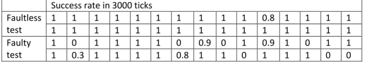
Table 3.1: Success rate comparison of faultless evolved controller in 3000 ticks ... 82

Table 3.2: Success rate comparison of faultless evolved controller in 1200 ticks ... 83

Table 3.3: Success rate comparison of faulty evolved controller in 3000 ticks ... 85

Table 3.4: Success rate comparison of faulty evolved controller in 1200 ticks ... 86

Table 4.1: Experiment index in terms of percentage deviation of cumulative mean result ... 105

Table 4.2: Baseline parameter values for evolution experiment ... 107

Table 4.3: U-test scores for the comparison between baseline and calibration values 116 Table 4.4: A-test scores for the comparison between baseline and calibration values 116 Table 4.5 Calibration parameter values for evolution experiment ... 117

Table 4.6: U-test score for three different MOCGPANN comparisons ... 118

Table 4.7: A-test score for three different MOCGPANN comparisons ... 118

Table 4.8: U-test score for four different crowding fill strategies comparisons with modified fitness function ... 122

Table 4.9: A-test score for four different crowding fill strategies comparisons with modified fitness function ... 122

Table 4.10: Result of number of experiment runs required from cumulative mean approach ... 123

Table 4.11: Success rate for generalisation experiment results in terms of robust fault tolerant control ... 125

Table 4.12: Success rate for generalisation experiment results in terms of switched fault tolerant control ... 126

Table 4.13: Comparison between the success rate of robust and switched fault tolerant control based on the controllers evolved by MOCGPANN ... 128

Table 5.1: Different aspects between NSGA2 and MOCGP for ANN evolution ... 137

Table 5.2: Baseline values for NSGA2 parameters ... 140

Table 5.3: Calibration values for NSGA2 parameters ... 140

Table 5.4: U-test scores for the comparison between NSGA2 parameter baseline values and calibration values ... 141

Table 5.5: A-test scores for the comparison between NSGA2 parameter baseline values and calibration values ... 141

(6)

v

Table 5.6: U-test and A-test scores for hyper-volume comparison between NSGA2 and MOCGP ... 143 Table 5.7: Success rate for five obtained Pareto sets by NSGA2 in terms of robust fault tolerant control ... 145 Table 5.8: Success rate for five obtained Pareto sets by NSGA2 in terms of switched fault tolerant control ... 147 Table 5.9: Comparison between the success rate of robust and switched fault tolerant control based on the controllers evolved by NSGA2 ... 148 Table 6.1: U-test scores for hyper-volume and generation number in terms of extension experiment ... 155 Table 6.2: A-test scores for hyper-volume and generation number in terms of extension experiment ... 155 Table 6.3: Result of number of experiment runs required from cumulative mean approach for the extension experiment ... 156 Table 6.4: Success rate for extension generalisation experiment results in terms of robust fault tolerant control ... 157 Table 6.5: Success rate for extension generalisation experiment results in terms of switched fault tolerant control ... 158 Table 6.6: Comparison between the success rate of robust and switched fault tolerant control based on the controllers evolved by MOCGPANN for this extension experiment ... 158

(7)

vi

List of figures

Figure 2.1: Fault accommodation (from [5]) ... 6

Figure 2.2: Controller reconfiguration (from [5]) ... 7

Figure 2.3: An example of GP genotype [17] ... 11

Figure 2.4: A simple feedback loop [17] ... 12

Figure 2.5: Block diagram of GP system design for MRAS controller [24] ... 17

Figure 2.6: An example of CGP genotype [30] ... 19

Figure 2.7: Migration topology of the used Parallel evolutionary algorithm [37] ... 25

Figure 2.8: A generalised artificial neuron model [30] ... 28

Figure 2.9: Feed-forward neural networks [44] ... 29

Figure 2.10: Recurrent networks [44] ... 30

Figure 2.11: Radial basis function neural networks [44] ... 30

Figure 2.12: Fuzzy neural networks [44] ... 31

Figure 2.13: An example of NEAT genotype and phenotype [62] ... 37

Figure 2.14: An example of two mutation ways of NEAT [62] ... 38

Figure 2.15: An example of crossover based on innovation number in NEAT [62] ... 39

Figure 2.16: An example of CGPANN genotype [30] ... 45

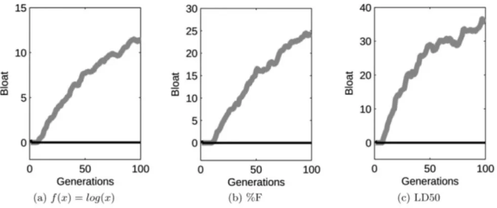
Figure 2.17: The comparison of GP and (gray line) and DynOpEq GP (black line) on (a) symbolic regression and (b) (c) two real world classification tasks in terms of program bloat investigation. [77] ... 47

Figure 2.18: Crowding distance calculation [92]. ... 61

Figure 3.1: Light sensor distribution of foot-bot [145] ... 77

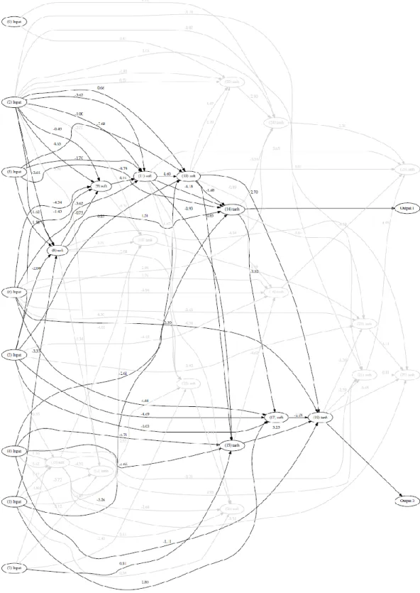
Figure 3.2: An example of CGPANN evolved controller without the connection to the failed sensor ... 79

Figure 3.3: Boxplot for success rate comparison of faultless evolved controller in 3000 ticks ... 83

Figure 3.4: Boxplot for success rate comparison of faultless evolved controller in 1200 ticks ... 84

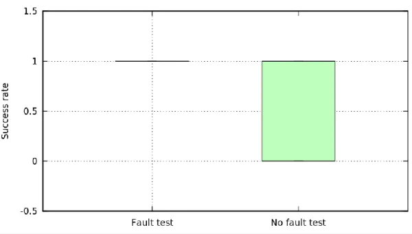
Figure 3.5: Boxplot for success rate comparison of faulty evolved controller in 3000 ticks ... 85

Figure 3.6: Boxplot for success rate comparison of faulty evolved controller in 1200 ticks ... 86 Figure 4.1: The evolved population from the final generation for one evolution run . 103

(8)

vii

Figure 4.2: The first Pareto optimal front solutions for the evolved population from the final generation for one evolution run ... 103 Figure 4.3: Hyper-volumes of baseline parameters ... 106 Figure 4.4: Number of generations of baseline parameters... 107 Figure 4.5: Hyper-volume comparison between baseline and calibration parameter values ... 116 Figure 4.6: Generation number comparison between baseline and calibration parameter values ... 116 Figure 4.7: Hyper-volume comparison for three different MOCGPANN ... 118 Figure 4.8: Generation number comparison for three different MOCGPANN ... 118 Figure 4.9: Hyper-volume comparison for four different crowding fill strategies with modified fitness function ... 121 Figure 4.10: Generation number comparison for four different crowding fill strategies with modified fitness function ... 122 Figure 5.1: Hyper-volume comparison between the NSGA2 parameter baseline values and calibration values ... 141 Figure 5.2: Generation number comparison between the NSGA2 parameter baseline values and calibration values ... 141 Figure 5.3: Hyper-volume comparison between NSGA2 and MOCGP... 143 Figure 6.1: Hyper-volume comparison for different crowding fill strategies in terms of extension experiment ... 154 Figure 6.2: Generation number comparison for different crowding fill strategies in terms of extension experiment ... 154

(9)

viii

Acknowledgements

Firstly, I would like to thank my parents Mr Chaoyi Zhang and Mrs Xiaodong Zhang for their support to let me finish my PhD course in the University of York. Especially, I would like to thank my wife Xiaotong Huang for her company with me during our life in UK.

Secondly, I would like to thank my supervisors Prof Jon Timmis and Dr Andy Pomfret as well as my internal examiner Prof Steve Smith for their help during my PhD study. In addition, I would like to thank our department graduate administrator Camilla Danese who helped me a lot whenever I got a problem during my work in our department. And then, I would like to thank my colleagues Guangsha Xu, Danesh Tarapore, Richard Redpath, Alan Millard and other people, who helped me a lot when I got stuck in my research.

Finally, I would like to thank all my friends I have ever made during these four years’ time in UK.

(10)

ix

Declaration

I declare that this thesis is a presentation of original work, which I undertook at the University of York during 2014 - 2018 and I am the sole author. This work has not previously been presented for an award at this, or any other, University.

(11)

1

Chapter 1

Introduction

1.1

Motivation

Fault tolerant control and evolutionary algorithms (EA) are two different research areas, yet have a natural synergy. With the development of artificial intelligence, EA has demonstrated competitive capability compared to traditional approaches for optimisation problems. In this case, the combination of fault tolerant control and EA shows great potential, with the ability to evolve new solutions that have the ability to adapt over time, and have greater potential for robustness to failure.

Typically, fault tolerant control based approaches employ EA to optimise the controller parameters for a given set of scenarios. However, the controller’s structure usually remains fixed when parameters are being optimised. Although the parameter optimisation based EA approaches have demonstrated effective performance for fault tolerant control, work in this thesis considers optimising the controller structure, in addition to the parameter space, with a view to observing a greater degree of fault tolerance.

1.2

Thesis contributions

The research question that this thesis aims to investigate is: “how can structure optimisation based EA approaches be utilised to evolve, at a structural level, fault tolerant robotic controllers?” In order to answer the research question, some main contributions are made in the thesis, which are:

 The review of literatures in fault tolerant control with structure optimisation based EA approaches and Cartesian Genetic Programming of Artificial Neural Networks is identified as the best suited controller structure optimisation approach used for designing a robot fault tolerant control system

 The investigation of how Cartesian Genetic Programming of Artificial Neural Networks could be utilised to design a robust fault tolerant control system  The review of survival selection along with population diversity and the

investigation of how it could be utilised to improve the crowding fill strategy for Multi-objective Cartesian Genetic Programming of Artificial Neural Networks

(12)

2

 The review of how hyper-volume indicator is used for performance measure and the investigation of how it could be utilised to assess the convergence for Multi-objective Cartesian Genetic Programming of Artificial Neural Networks  The development of a complete library of Multi-objective Cartesian Genetic

Programming of Artificial Neural Networks based on a new crowding fill strategy and the investigation of how it could be utilised instead of single objective optimisation to obtain a Pareto set of controllers used for the design of a robust as well as switched fault tolerant control system

 The investigation of how Non-dominated Sorting Genetic Algorithm 2 could be utilised to design a robust as well as switched fault tolerant control system based on multi-objective controller parameter optimisation

 The comparison between Multi-objective Cartesian Genetic Programming of Artificial Neural Networks and Non-dominated Sorting Genetic Algorithm 2 for controller evolution in order to investigate the difference between controller structure optimisation and controller parameter optimisation

 The investigation of how Multi-objective Cartesian Genetic Programming of Artificial Neural Networks could be utilised to design a robust as well as switched fault tolerant control system based on multi-objective controller structure optimisation for a more difficult fault tolerance scenario

1.3

Thesis outline

This section gives an outline of each chapter for the remaining thesis summarised as below:

 Chapter 2 reviews fault tolerant control and different structure optimisation based evolutionary algorithms along with artificial neural networks in order to find out a suitable approach to design a fault tolerant control system. Moreover, different multi-objective optimisations are also reviewed and survival selection based on crowding measure is also mentioned along with population diversity. Finally, convergence criteria and statistics analysis are both introduced.

 Chapter 3 presents how Cartesian Genetic Programming of Artificial Neural Networks, which is the approach obtained in chapter 2, is utilised to achieve the robust fault tolerant control.

(13)

3

 Chapter 4 demonstrates how genetic redundancy and crowding measure along with hyper-volume indicator are utilised to develop the library of Multi-objective Cartesian Genetic Programming of Artificial Neural Networks and displays how it could be utilised to achieve both of robust and switched fault tolerant control.

 Chapter 5 shows how Non-dominated Sorting Genetic Algorithm 2 could be utilised to evolve feasible controllers so as to achieve both of robust and switched fault tolerant control and presents how it is compared with Multi-objective Cartesian Genetic Programming of Artificial Neural Networks for the evolution experiment performance.

 Chapter 6 presents how Multi-objective Cartesian Genetic Programming of Artificial Neural Networks is performed to achieve a more difficult fault tolerant control scenario for both of robust and switched fault tolerant control.  Chapter 7 gives a summary about the thesis and the proposed future work.

(14)

4

Chapter 2

Literature review

2.1

Introduction

The aim of this thesis is to fill the research gap that controller structure optimisation based EA approach has not been investigated as the same level as controller parameter optimisation for fault tolerant control. In this case, the thesis will explore how controller structure optimisation could be utilised to design a fault tolerant control system. For this reason, this chapter will review the area of fault tolerant control firstly and then review how different structure optimisation based EA approaches have been performed in the controller structure optimisation tasks. This chapter will also estimate the respective benefit and drawback for different structure optimisation based EA approaches along with an investigation of artificial neural network for the controller type in order to find out the most suited approach to be utilised for the design of a fault tolerant control system.

2.2

Fault tolerant control

Faults in automated processes will usually cause undesired results especially the shut-down of controlled plants. These consequences could be harmful to the plant, to personnel or the environment. In this case, fault tolerant control was developed which is used to increase the plant availability and reduce the risk of safety hazards so as to avoid a simple fault becoming a serious failure [1].

Fault tolerant control can be classified into two aspects: passive or active [2]. Passive fault tolerant control uses a specific fixed controller to be robust against certain faults [3]. And active fault tolerant control redesigns the control system in order to maintain an acceptable performance after a fault occurs [4]. In active fault tolerant control, [2] indicates two necessary tasks: fault detection and isolation and fault accommodation or controller reconfiguration. Fault detection and isolation consist of a fault diagnosis scheme and fault accommodation or controller reconfiguration can be regarded as controller redesign [5]. Active fault tolerant control has more fault tolerant capabilities than passive fault tolerant control just equipped with a robust controller [6]. Because there will be more solutions to cover more classes of faults if the controller can be changed [7].

(15)

5

means that the dynamic structure and parameters of the controller will change to accommodate the fault, but the relationship between controller and plant still maintains fixed including the reference signal and control value. So the fault can be accommodated only if the controller has a solution to deal with the faulty system [4]. Although fault accommodation can be quick to find a suitable controller in order to realize some hard real time constraints [5], the controllers need to be pre-designed for all the possible types of faults. So the fault accommodation cannot work well if no solution is found among the controllers especially the relationship between controller and plant needs to be adjusted if a degraded performance has to be accepted in some cases. On the other hand, controller reconfiguration will establish a new control loop including a reconfigured controller with the introduction of alternative input and output signals between the controller and the plant [7]. In this sense, the controller can be reconfigured online to achieve the performance of different faulty systems including some degraded performance. However, the controller reconfiguration emphasizes the parameter reconfiguration based on some optimization techniques [2], so the research of controller structure reconfiguration is still in an early stage. Although the evolution of controller structure has been studied, this research field hasn’t been put into the fault tolerant control scheme. Therefore the hypothesis of this work can be described that the fault tolerant control can work better if the controller structure evolution is associated with the controller reconfiguration.

2.2.1

Passive fault tolerant control

In the field of passive fault tolerant control, the robust control is the main approach [2]. It designs the controller with constant parameters as well as the structure to correct a specific fault so as to guarantee the required performance [7]. And the control objectives of robust control mainly include the following fields: stability, disturbance rejection and noise rejection [8]. Typically the most effective way of robust control is to cope with the faults which can be modelled as plant uncertainties [7]. For example, [9] designs a robust control system against the plant uncertainty. This work belongs to a kind of model following control which uses a correction mechanism to cope with the deviations between the real plant and the reference model to achieve the reference tracking task. The reference model reflects the expected performance of the plant and the correction mechanism is used to force the plant to follow the model. However due to the parameter variations or system disturbance, the uncertainty is always a problem occurred in the real plant. So the correction scheme is designed equivalently as a

(16)

6

controller to control the plant in the worst case of uncertainty [9]. This work is a typical example to apply the robust control scheme to cope with the system uncertainty. So the effectiveness of the passive fault tolerant control emphasizes on the robustness of control system against certain faults as well as the disturbance and noise in the system with fixed controllers. However, this approach has limited fault tolerant capabilities with just robust controllers [6]. Therefore if the controller can be changed, there will be more solutions to cover more classes of faults compared to the passive approaches [7]. So that’s why the active fault tolerant control was developed.

2.2.2

Active fault tolerant control

In the research area of active fault tolerant control, [5]mentions two tasks: fault diagnosis and controller redesign. Fault diagnosis means an early detection, isolation and also identification of faults. And controller redesign needs to be performed after the fault is diagnosed to achieve fault tolerant control. Controller redesign contains two main approaches: fault accommodation and controller reconfiguration which are respectively shown in Figure 2.1 and Figure 2.2.

(17)

7

Figure 2.2: Controller reconfiguration (from [5])

In these two figures, f is the fault, is the reference input, u is the control value, y is

the system output, , and are the corresponding new signals. These two

approaches both need to change the parameters and structures of controllers to avoid the consequences of faults. However the difference is that controller reconfiguration needs to change the input and output signals between the controller and system so that a new control loop will be generated. But the fault accommodation maintains the same values for all the signals [5].

 Fault accommodation

In fault accommodation, one of the representative approaches is the switched control. It is based on the bank of controllers designed for the normal and different faulty systems [5]. The pre-designed controllers are generated offline to process different types of faults. So their internal structures may be different, but the I/O signals will remain the same to achieve accommodation [7]. Therefore it is a switching mechanism that a suitable controller needs to be selected in terms of the type of fault. The benefit of fault accommodation is that it can be quick to find a suitable controller so that some strong real time constraints could be realized [5]. However this approach needs to pre-design the controllers for all the possible types of faults. If none of the pre-pre-designed controllers is available to deal with a typical fault, the required performance cannot be achieved.

(18)

8  Controller reconfiguration

In controller reconfiguration, a new control loop is established with the introduction of alternative input and output signals between the controller and the system [7]. This approach could be applied when a fault is occurred in the system sensor or actuator. In this sense, a new control loop with a new controller and alternative signals needs to be established when alternative components are introduced [5]. This approach is able to process unplanned faults by changing the new control objectives and constraints, so a new control loop is also required. However designing a new control system based on a new control loop is definitely not an instant work, so the controller reconfiguration would be more suited to the tasks where sufficient time is allowed to designing a new control system during the system operation.

As can be seen from these two approaches, fault accommodation and controller reconfiguration have their own benefits and drawbacks. Actually fault accommodation refers to the offline designing controllers where the controllers need to be designed well before loaded to the real system. However controller reconfiguration always refers to the online designing controllers where the controllers are being designed during the system operation. In this case, the fault accommodation can guarantee that the controller will be working well since it was well designed offline. However controller reconfiguration cannot ensure when the controller design is finished before loaded to the system in order to avoid a crashed system. On the other hand, fault accommodation has to design all the possible types of controllers offline, if a unplanned fault occurs online, there is no way to tolerate this fault. However, controller reconfiguration is capable to deal with all the possible types of faults including unplanned one as long as the fault can be diagnosed. In conclusion, fault accommodation and controller reconfiguration both have benefits and drawbacks. Therefore, which one to be utilised for fault tolerant control is dependent on the difficulty of the given task including the passive fault tolerant control approaches.

2.3

Evolutionary algorithms in controller structure optimisation

2.3.1

Introduction of evolutionary algorithms

EA is a kind of optimization algorithms in the artificial intelligence area which was developed based on the inspiration of natural selection and survival of the fittest in Darwinian evolution [10] [11]. Generally speaking, there are several steps to constitute

(19)

9

a complete evolution loop. Firstly, the initial population needs to be created randomly as the first generation. Secondly, this population needs to be evaluated for the given problem and their performance is recorded as fitness values where the given problem is normally called fitness function. After that, this population needs to be selected based on the fitness value and the selected parents will be utilised to create their children for the next generation based on genetic operator including crossover and mutation. And when the children are obtained, they also need to be evaluated based on the fitness function. Now it comes to the crucial step called survival selection. In the survival selection, one option is just utilising the children as the next generation, which is easy and straight forward for many EA applications. The other will compare the obtained children with their parents. If children’s fitness is not better than the parent, the parents will be directly copied into the next generation without any change, which is also called elitism strategy. However whether elitism is required depends on the given task since elitism will not always be the suited idea to obtain the new blood for the next generation. Nevertheless, one significant benefit of elitism is that it always guarantees the next generation to be at least performing equivalent as the last generation, which is convenient for convergence observation and helps to achieve a better convergence especially for multi-objective EA (MOEA) [12]. The above is a whole evolution loop and EA will only stop when termination condition is met such as the target fitness value is obtained, the maximum generation number is reached or the convergence criteria is realised [10] [11].

In terms of fault tolerant control, genetic algorithm (GA) based approaches have been investigated extensively. GA is used as an optimization tool that the task is normally about how to optimize the parameters of a controller to deal with different types of faults [2]. For example, [13] designs a fault tolerant control system for an active magnetic bearing task using a multi-objective GA. In this work, the active magnetic bearing system is used to tolerate the faults occurred in a coil or an amplifier in a machine. To design an active magnetic bearing system, PID controller is applied with multi-objective GA to tune the parameter of the PID controller to achieve different configuration of this active magnetic bearing system.

This work shows a typical example of using GA as an effective approach to tune the parameters of controllers to achieve the fault tolerant control. However, GA is just one of the simplest EA which can be only used for the parameter reconfiguration so that

(20)

10

the controller structure always maintains fixed. If the controller structure could also be changed, more solutions might be generated to deal with more types of faults. However controller structure optimisation hasn’t been developed as the same level as controller parameter optimisation in the fault tolerant control area and that’s why the combination of controller structure optimisation with fault tolerant control would be a new research topic. On the other hand, active fault tolerant control needs rigorous identification of all classes of faults so that the controller redesign could be carried out [14]. Therefore the controller structure configuration could also be a promising approach to deal with a wider range of faults as long as the fault could be diagnosed. For this reason, there are some other EA approaches which were developed to work for the optimisation of the structure as well as the parameters. Those structure optimization based EA approaches are reviewed in the following sections.

2.3.2

Genetic programming

Genetic programming (GP) is a kind of structure optimisation based evolutionary algorithms (EA) approach which is normally used to automatically create a computer program to solve a problem using program trees [15]. GP was firstly introduced in [16] based on the parse trees as the genome encoding in order to create programs. In this kind of tree based GP, the computer programs are created in tree structures where a tree node is an operator such as [+, -, *, /] and the terminal node is a variable such as [a, b, c, d]. Based on this tree structure, the programs will be evaluated for each generation and the evolution will be finally terminated when an acceptable program expression is found. In this case, Lisp became the first programming language applied to this tree based GP since Lisp is also expressed in a tree structure that matches the genotype of this tree based GP. In terms of the genetic operator, there are two different types applied for the mutation including the point mutation and sub-tree mutation. Point mutation randomly changes the functions or terminals of a proportion of the nodes within a parse tree and the number of nodes are determined by the mutation rate. Sub-tree mutation randomly changes the whole sub-tree to a new one with randomly selected functions and terminals. On the other hand, sub-tree crossover is the only type for crossover which creates two children with the swapped two sub-trees from the selected two parents [16]. An example of tree based GP genotype is shown in Figure 2.3.

(21)

11

Figure 2.3: An example of GP genotype [17]

Besides the basic approach of GP to write a computer program, the program trees can be also interpreted to construct a complex structure, such as an electrical circuit [18]. Moreover, the program trees could be interpreted to represent the block diagram of a controller so as to achieve the controller evolution [15]. In this research field, several related works are reviewed as following including control system design and robotic controller design based on GP. Among these works, [17] presents a typical implement of how to use GP to evolve a controller so as to design a control system, so this work will be described in more details.

 GP for control system design

[17] considers a simple feedback control loop to be used for controller evolution which is shown in Figure 2.4. In this control loop, the process is a continuous time dynamic system, the controller is also a dynamic system with unknown structure and parameters, y is the controlled variable, r is the reference variable, u is the control variable, e is the control error.

(22)

12

Figure 2.4: A simple feedback loop [17]

In this case, a simple integral performance index is chosen as the cost function which is defined in equation 2.1 where T is the simulation time and ̇ is the controlled variable derivative. ∫|e(t)|dt T 0 ∫|ẏ|dt T 0 (2.1) The aim of controller design is actually an optimization task which searches for a controller so that the chosen performance index could be minimized [17]. This cost function consists of two parts. One is a basic integral absolute error (IAE) form which integrates the absolute error over time in order to minimize it. The other is described in a form of integral absolute output derivative multiplied by a coefficient. It could be used to minimize the output slope over time so that the output trajectory could become smoother with an appropriate choice of the coefficient.

To demonstrate the performance of GP, two different case studies are implemented in this work including a continuous time and a discrete time controllers design. The first test case uses a continuous time interconnected network to describe the control algorithm with a table based representation of individuals which is different from classical tree based representation in GP. The function blocks include integrator, derivative unit, amplifier (multiplication by a constant) and summation/multiplication unit. The objective is to find an optimal controller network with these function blocks which minimizes the above cost function. The crossover used here will exchange the corresponding parts of two random positions between two columns of the table. And mutation will change the type of block or delete and add a block or change the value of a constant [17]. In the second test case, a discrete time recurrent control algorithm is designed with a classical tree representation of genotype. The crossover exchanges the

(23)

13

randomly selected sub- trees from two trees and the mutation replaces a randomly selected sub-tree by another one. To demonstrate the effectiveness of using GP for controller design, two linear dynamic systems are implemented, which are shown in transfer function 2.2 and 2.3.

( ) (2.2) ( ) ( ) (2.3) The optimization results and algorithm running time of obtained controllers of two linear dynamic systems are demonstrated in Table 2.1 compared with the results of a PID controller tuned by GA for the first system. GP1 means the table based continuous time controller, GP2 means the tree based discrete time controller and GA PID means GA based PID controller.

Table 2.1: The obtained results for two different linear dynamic systems [17].

Experiment 1 Cost function value Time

GA PID 11268 3h55min

GP 1 3950 18h57min

GP 2 12265 5h53min

Experiment 2 Cost function value Time

GP 1 6509 20h27min

GP 2 19646 5h24min

As can be seen from the Table 2.1, GA PID has the fastest running time but high cost function values. GP1 achieves the lowest cost function values but much slower running speed. And GP2 has similar results compared to GA PID and higher cost function values and faster running time compared to GP1. So the table form based GP method could be a promising approach due to its obvious benefit of lowest cost function values compared to GA tuned PID controller. However the running time of this approach is much longer than the other two approaches and this issue needs to be improved. According to the performance index, GP1 obtains the best dynamic performance which has the shortest rise time and settling time with no overshoot for the first system. In

(24)

14

terms of the second system, GP1 is also better than GP2 with slightly faster rise time, shorter settling time and lower overshoot.

As can be seen from this work, GP is capable to find acceptable solutions for controller design based on the feedback closed loop, which outperforms the GA based PID controller. Furthermore, table based GP also produces better performance than classic tree based GP, which indicates that the tree based GP may not be a first choice depending on the given task in spite of a shorter running time. Finally, this work also notes that GP can be used to design the controller with complex systems, but the only limitation is the high requirement of computation time, which may be a common issue for GP based approaches.

 Improvement of GP based control system design

Besides a description of how to use GP to construct the controller [17], there are also some approaches to improve the performance of GP based controller design. According to [19], GP can be used to construct a discrete recursive feedback control law using the equation 2.4.

( ) ( ) [ ]

(2.4) For a population size of M the output of the ith {i 1,2,3…M} controller at time k is equal to the output at time step k-1 plus some correction term applied by the ith GP individual. The fitness function is shown in equation 2.5. This is calculated using P independent and randomly generated set point changes: △ {j 1,2,3…P}.

∑ ∑ | ( )| ( )

(2.5) In 2.5, n is the number of discrete time steps which is decided by trial and error before GP runs. k|e(k)| is the integral time absolute error (ITAE) term and ( ) is a weighted penalty term for excessive control effort u(k) with a constant r determined by trial and error [19]. This fitness function minimizes two aspects of the controller performance which are the error and the controller output. Although the output slope

(25)

15

is not minimized here which is mentioned in [17], the excessive control effort could be decreased in this case. To demonstrate the effectiveness of this approach, [19] uses two chemical processes for controller design including a constrained second order ARX(auto-regressive exogenous) process and a non-linear CSTR(continuous stirred tank reactor) process. The ARX process is defined in equation 2.6. And the non-linear dynamic model of CSTR is referred from [20].

( ) ( ) ( ) ( ) ( )

(2.6) As can be seen from the ARX process response comparison, the evolved controller has longer rise time than the PID controller but without any overshoot. While for the settling time, they have similar performance. And according to the CSTR process response comparison, they both perform similarly just the evolved controller has slightly larger overshoot. Therefore, GP is capable of producing dynamic recursive controllers which provide similar performance compared with PID controllers [19]. Hence the concept of recursive feedback control law used in GP could be applied to the controller design in the discrete time domain. Although its performance is similar to PID controller, it is still an encouraging idea to use GP for the discrete controller design. [21] also improves the performance of GP based controller design by creating a controller with a free variable. The reason to introduce a free variable in the controller design is that the evolved controller could control an entire category of plants through modifying the value of the free variable instead of a particular plant with a fixed variable. The tree format is used to present the controller. A three-lag plant is used for the controller design and the controller contains a free variable representing the plant time constant τ. This free variable can be changed among 0.1, 0.3, 1.0, 3.0 and 10.0 which are defined in this work. In this sense, the evolved controller becomes a function of this free variable which corresponds to the plant time constant. The transfer function of this three-lag plant is defined in equation 2.7 where K is the plant’s internal gain(tested by values of 1.0 and 2.0) [21].

( )

(26)

16

The fitness is measured by means of 42 separate fitness measurements. Among these 42 fitness measurements, the first 40 are based on a modified integral of time-weighted absolute error (ITAE) which is shown in equation 2.8 where e(t) is the error;

is the externally supplied value of the time constant; B is a constant; A is an additional weight value which varies depending on the error so that unacceptable overshoot could be avoided; and finally each integral value needs to be divided by so as to equalize the influence of five different values of . The 41st One is in frequency domain which constrains the frequency of the control value to avoid extreme high frequencies applied into the plant. The last one is also in frequency domain measuring the effect of sensor noise.

∫ | ( )| ( ( ))

(2.8) This obtained controller is compared with the Astrom and Hagglund controller which is a PID controller tuned with a new simple tuning rule by Astrom and Hagglund [22]. As can be seen from the result, [21] calculates that the controller created by genetic programming is better than 3.69 times as effective as the Astrom and Hagglund controller as measured by the integral of the time-weighted absolute error(ITAE), has only 57% by the rise time, and has only 55% by the settling time. Moreover, the genetically evolved controller is more robust to the disturbance than Astrom and Hagglund controller indicated from the disturbance sensitivity. The computation time to find the best of run evolved controller is 23.43 hours. The conclusion demonstrates that GP can be used to create a controller with a free variable which outperforms Astrom and Hagglund controller [21]. Therefore the evolution of robot controller could be referred to this approach using a free variable in the controller design. Although this approach has much better performance than the Astrom and Hagglund controller, its computation time of 23.43 hours is still high.

 GP based robust controller design

GP can be also used to construct a robust controller. [23] applies GP to construct a robust flight controller against the wind shear. The occurrence of strong downbursts could cause serious crashes of landing aircrafts. So the problem is how to construct a

(27)

17

robust flight controller with GP to make the aircraft land along the reference trajectory:

in the case of wind shear. The performance of the generated controller is illustrated using the aircraft trajectories in terms of different sizes of wind shear. The result shows that the GP based robust controller could achieve effective performance for aircraft to be landed safely in spite of different sizes of wind shear. Therefore this work describes another application of GP in the robust controller design, and the results show that GP is able to get effective solutions.

 GP for tuning controller parameters

[24] describes the application of GP to tune a controller parameters. In this work, GP is used to construct a self-evolved Model Reference Adaptive System (MRAS) which is designed for a second order system based on a pre-defined reference model. MRAS is one of the adaptive controllers, its performance is described through a reference model which gives the desired response to a reference signal [25]. The aim of this work is to evolve a suitable controller which is based on the desired model to control a process. Actually this work applies GP to automatically tune the controller to meet the desired performance. Because the structure of the controller is already given, so the work of GP is to provide the correct controller parameters [24]. The block diagram of this work is shown in Figure 2.5.

Figure 2.5: Block diagram of GP system design for MRAS controller [24]

In this diagram, uc is the controller input, u is the plant input, y is the plant output, ym is the model output and e is the error between the model output and the plant output. Although this work doesn’t use GP to evolve the structure of a controller, it presents another approach of GP to generate the controller parameters. According to the

(28)

18

conclusion of [24], GP is able to generate desired parameters of MRAS controller based on the model following without any prior knowledge about the system parameters [24]. Therefore this work presents another application field of GP for the controller parameter generation and GP is also able to find acceptable solutions.

 GP in the evolution of robotic controller

Apart from the controller design, GP can be also used for the evolution of robotic controllers [26] [27] [28]. [26] uses GP to achieve a robot reactive navigation task. The aim of GP is to evolve the best trajectory that the robot follows the environment without bumping into a wall. [27] uses GP to achieve the task of wall-following for a robot. In this work, different types of walls are tested for GP to evolve the acceptable solutions of robot behaviours without priori information about the environment. [28] also uses GP to evolve a robot behaviour controller. The aim of GP is evolving an appropriate relation between the sensor terminals and motor commands in order to manage the robot to achieve desired behaviours. Therefore two tasks are applied for GP to get acceptable controllers which are obstacle avoidance and box-pushing. Obstacle avoidance is to make the robot not bump any obstacle and box-pushing is to keep the robot pushing a box forward as straight as possible [28]. The results of these three works all show that GP can get good behaviours for a robot task based on the evolution of a robotic controller. Although they are not related to typical controller design problems in control theory area to realise dynamic performance index as well as the steady state error of static performance index, these works still present another application area of GP to achieve the robotic controller design. Moreover, GP is also suited to the multi-input multi-output (MIMO) controller design problems for robotics where the sensor readings can be used as the controller input values and the controller output values actually stand for different motor speeds, where a standard single input single output (SISO) controller is not able to achieve. In conclusion, the GP based robotic controller evolution is a promising way to achieve the robot behaviour management so as to achieve different robot tasks. In this sense, it would be interesting to investigate it into the robot fault tolerant control area and explore how it will be working.

(29)

19

2.3.3

Cartesian genetic programming

Cartesian genetic programming (CGP) is another type of GP which uses a two-dimensional grid of nodes to represent a program rather than the tree form used in GP [29]. In terms of the CGP genotype, each one is described with a directed acyclic graph of computational nodes. An example of CGP genotype is shown in Figure 2.6.

Figure 2.6: An example of CGP genotype [30]

The genotype of CGP consists of function genes, connection genes and output genes. One advantage of CGP over GP is that the node outputs can be reused more than once without recalculating the same required value, which can be seen in Figure 2.6. Another advantage is that CGP is quite suited to MIMO problems with the specified number of inputs and outputs. Moreover, CGP also does not suffer from program bloat problem and the details can be referred to section 2.4.4.2. Finally, CGP is also benefit from the inactive genes, where the details can be referred to section 2.4.4.5. Basically, CGP utilises (1+4) for the evolutionary strategy with point or probabilistic mutation. Point mutation changes the randomly selected genes with a fixed amount, which is determined by the total number of genes times the mutation rate. In terms of the probabilistic mutation, each gene will get a chance to be mutated based on a given mutation rate. Apart from the mutation, there is however no crossover utilised for CGP. A possible reason is that using crossover for CGP has not generally demonstrated any advantage for a wide range of task domains [30].

In terms of the CGP applications, three different fields are described which are related to CGP based controller design tasks. [31] and [32] are directly related to how to design a control system by CGP for two different nonlinear systems, so they will be discussed in more details. [33] is about how to evolve a robotic controller based on the relations between the input sensor signals and output motor speed of the robot. And [34] is

(30)

20

about how to evolve the input signals of a motor controller to achieve sensor fault tolerant control.

 CGP for control system design

The work in [31] demonstrates that CGP can be also used for control system design besides the basic GP approach. [31] mentions that the computation time for GP based approach is extremely high so that an acceptable solution could take days of time to be evolved for a simple SISO controller design. So CGP is considered to be an alternative way with some limitations or simplifications in the task definition such as the orthogonal network for the individual representation. Since the interconnection of the nodes in this kind of network is not arbitrary as GP, so the solutions with much lower computation time could be obtained due to the reuse of nodes for the program description [31]. In this approach, CGP is used to design a controller for a nonlinear hydro-turbine system whose model can be referred to [35].

According to [31], each individual contains N interconnected building blocks where each block consists of three parts: the arithmetic operators (summation, subtraction, multiplication or division), the gain and the dynamic operators (integrator, derivative or unit gain). And the interconnection number between the controller inputs, building blocks and controller output is limited to M. N and M are priori determined based on the complexity of the system. So an appropriate selection of N and M by the designer will maximize the controller performance [31].

The fitness function is presented in the form of integral absolute error (IAE) which is defined in equation 2.9 where T is the simulation time.

∫| ( )|

(2.9) This fitness function is just used to minimize the error between the reference signal and output signal. In this sense, unstable individual will be eliminated due to their high performance index. Moreover, a GA designed PID controller is also utilized as a comparison with CGP controller for the same problem.

(31)

21

As can be seen from the result, CGP designed controller achieves shorter rise time, shorter settling time and lower overshoot compared with GA tuned PID controller. And with the increase of generation number, CGP approach can get a lower cost function values compared with GA approach. The conclusion in [31] indicates that CGP is effective to obtain acceptable controller design result. And it uses additional limitations related to the controller structure and its size to reduce the computation effort compared to GP. In the future work, CGP can be used for controller design with complex MIMO and any type non-linear systems [31]. Therefore CGP based controller optimization could be a useful approach to design a control system. The only condition to apply this method is the existence of a suitable model of the controlled system [31]. As long as the system model is obtained and sufficient computation capacity is given, this approach is a promising method to obtain acceptable controllers.

[32] also uses CGP for the controller design of nonlinear system. This work uses a different system to demonstrate the ability of CGP to design acceptable controllers. [32] conducts an explicit comparison between CGP and GP. In terms of CGP, it has an exclusive limitation which defines the individual structures that the building blocks are normally organized in a fixed grid with a priori defined size and the task is to find the optimal types, parameters and interconnections among them. However GP generates the individuals with unlimited structures. So the limitation of GP is just the number of building blocks or the size of program tree or table [32].

The individual representation and fitness function of [32] is the same as [31]. The controlled system of [32] is a SISO system which is described by a differential equation in 2.10 where y is the system output value and u is the control value. Furthermore, a GA designed PID controller is also implemented as a comparison with CGP designed controller for the same system.

(2.10) As can be seen from result, CGP approach can get controllers with acceptable performance while GA tuned PID controller has the problem of steady state error and even cannot reach the reference value when it changes. Therefore the conclusion of

(32)

22

[32] points out that PID controller doesn’t meet the requirements of all the different references for the time response due to its linear behaviour and insufficient robustness. However CGP controller is able to reach the reference value in an entire range. Although it is difficult to obtain the optimal controller because of the huge search space, this approach can still produce acceptable solutions [32]. In conclusion, [31] and [32] use two different systems to demonstrate the effectiveness of CGP to obtain acceptable controllers compared with GA tuned PID controller, which also indicates that CGP is capable to design a nonlinear control system based on the controller optimization.

 CGP in the evolution of robotic controller

Apart from control system design in the control theory field mentioned in the above two works, Cartesian genetic programming can be also used to generate controllers to manage robot behaviours [33] in addition to the GP based robot controller evolution [28]. In this work, the nodes from the first column of the evolved controller consist of two sensor inputs and two nodes from the last column stand for two motor speeds. The following functions can be selected for the nodes including Add, Subtract, Multiply, Divide, Compare, Min, Max, Fixed integer and Input node. The fitness functions are developed based on these factors such as time spent moving forward, total path length and Euclidian distance travelled [33]. Based on the utilizing of CGP, this work successfully creates controllers for two experiment tasks, which are escaping a room and solving a maze. As can be seen form this work, the approach could evolve a controller which constructs relations between the inputs of sensor values and outputs of motor speeds to complete the robot tasks such as obstacle avoidance and maze solving for robotic controller design mentioned in this work. What’s more, this kind of controller evolution based on CGP is quite suited to the MIMO controller design problems especially in robotic area since it could evolve a MIMO controller which utilizes the sensor readings as the controller inputs and creates controller outputs for each of the motor speeds respectively. In this case, this kind of MIMO controller will be working well to manage the robot behaviour rather than a typical SISO controller which is just designed on the utilize of the error as the unique controller input to generate an output value as the control signal to control the plant. In conclusion, this work indicates an interesting area of using CGP to evolve robotic controllers to manage robot behaviour to achieve different robot tasks. Based on this work, it would be interesting

(33)

23

to consider evolving controllers to achieve robot fault tolerant control as long as the fault has been diagnosed.

 CGP in fault tolerance

[34] tries to use CGP to achieve sensor fault tolerant control. This work is related to controller design in the case of a sensor fault. However it is not about designing a controller, it is focused on how to generate the correct inputs to the controller using CGP with the remaining working sensors [34]. The controlled system is the Shaky Hand plate. The inputs of CGP are the plate sensor signals and the outputs will be the lateral and angle offset error voltages which are the inputs of controllers and used to drive motors to compensate for them. Therefore the aim of CGP is to generate the relation between the remaining working sensor signals and two offset error voltage values [34]. As can be seen from this work, CGP is still effective to search for reliable solutions for the sensor fault tolerant control. Although this work is not about the controller evolution, it indicates a new idea to evolve the inputs of controller which could also be helpful for fault tolerant control.

2.3.4

Grammatical evolution

Grammatical evolution (GE) is also another type of GP. It can evolve a program using arbitrary languages with a variable-length binary string. This binary genome determines which rule in the grammar is used to achieve the mapping from genotype to phenotype so that the program could be completed. Basically, Backus-Naur Form (BNF) is utilised as the original grammar rule employed for the mapping based on the building blocks in order to create the potential program. However, any language could be created based on this kind of simple binary string as long as an effective mapping process is available to implement [36].

In terms of GE applications, [37] presents a whole scheme about how to use GE to evolve a controller to design a control system and [38] talks about how to use GE to evolve a robotic controller for robot behaviour management.

 GE for control system design

According to [37], grammatical evolution can be used for controller design for arbitrary continuous time dynamic systems. The controller is represented in a continuous time

(34)

24

function which includes the selected arguments , the mathematical relations and the parameters of the mathematical operations. The arguments of input variables are

where e is the control error, ie is integral of control error, de is derivative of e, r is the reference signal, y is the controlled value and other arbitrary variables. The individual can be represented in 4n genes:

where is the code of a mathematical operation, is the argument of input variables, is the parameter representing the coefficient of each and is the coefficient of the power operation. The grammar of the mathematical operation is in the coding:

( ) ( ) ( ) ( ) ( ) where

The fitness function is in a form of simple integral performance indices defined in equation 2.11 or 2.12 where T is the simulation time.

∫| ( )|

(2.11)

∫| ( )| ∫| ̇|

(2.12) A parallel evolutionary algorithm [39] is used in this work which is illustrated in Figure 2.7.

(35)

25

Figure 2.7: Migration topology of the used Parallel evolutionary algorithm [37]

In simple population of EA, this is always a conflict between the selective pressure and population diversity. Therefore by introducing multiple populations in parallel evolutionary algorithm, it is possible to simultaneously increase the selective pressure in some populations and improve the diversity of other populations [39]. In this kind of parallel EA shown in Figure 2.7, the individual representation is described using 9 islands in parallel architecture which are interconnected with migration connections and each island contains 50 individuals. It is a hierarchical structure that island 1 is the upper-level node while others are low-level nodes. Hence the difference between this kind of parallel evolutionary algorithm and the simple population evolutionary algorithm is the migration that in each generation, the best individual from island 2-9 will be selected and copied into the island 1 [37].

A non-linear stable controlled object is used for GE based controller design which is displayed in a differential equation 2.13. As a comparison, GA designed PID controller is also utilised for the same system.

̈ ̇

(2.13) As can be seen from the result, GE based controller has a faster rise time than GA based PID controller in terms of system output. And GA based PID controller also causes some oscillation when the reference signal drops to 0. Moreover, GA based PID controller generates much higher control value than GE based controller which means

(36)

26

PID controller needs more control effort to control the system. In conclusion, the result demonstrates that GE is an effective approach which could generate more effective controller than GA tuned PID controller.

On the other hand, a non-linear unstable system is also used for the design of GE based controller which is described in a differential equation 2.15.

̈ ̇

(2.15) According to the result, GA based PID controller leads much higher overshoot of system output than GE based controller. In addition, GA based controller generates much higher control value which means more control effort is required for GA based PID controller than GE based controller. In conclusion, the result also demonstrates that GE designed controller achieves better performance than GA tuned PID controller.

According to this work, the GE based controller has obvious advantages for the control of non-linear system due to its non-linear properties of the controller compared to GA based linear controller. The future research of this approach will design the controller for complex, non-linear and MIMO systems. On the other hand, this approach just uses five mathematical operations which are {+, -, *, /, ^}. In this case, more kinds of operations and functions can be considered to be added into the individual representation if they are needed. In summary, [37] demonstrates that GE is an effective approach to construct acceptable controllers to deal with nonlinear systems, which could be an effective approach for control system design.

 GE in the evolution of robotic controller

Similar to GP based robot controller evolution [28] and CGP based robot controller evolution [33], [38] also describes how to evolve a controller to achieve robot task but with GE. In this work, the task is navigating a robot toward a point light source and avoiding obstacles at the same time. The evolved controller by GE is a piece of computer program that generates C code in order to make robot achieve the task. The obtained program maps a relation between the sensor signals and the motor speeds in order to control the robot behaviour. The genotype is evolved using a steady state GA where only a small part of population is replaced each generation. The only difference

(37)

27

is that the genomes in GE are represented in computer programs rather than binary or real values in GA for only evolving parameters. The fitness function is designed with two factors including a reward for finding a light and a penalty for collisions [38]. As can be seen from this work, it is quite similar to [28] and [33] where the evolved controllers are suited to solve MIMO controller design problems especially in robotics research area, which is also a potential way to achieve the robot fault tolerant control.

2.4

Evolutionary algorithms with artificial neural networks

2.4.1

Artificial neural networks

2.4.1.1 Introduction of artificial neural networks

Based on the reviewed literatures, EA is an effective optimization tool to design structurally evolvable controllers not only for SISO control problems but also for MIMO control scenarios. As can be seen from [28], [33] and [38], structurally evolvable EA approaches could also be promising to design controllers in terms of robot behaviour management. Although these approaches demonstrate benefits to design structurally evolvable controllers, those evolved controllers are created based on stochastic initial structures. That is to say, the output values of the controllers are actually arbitrary depending on which node functions are utilised and connected to the controller outputs. However the robot motor speed has the upper and lower limitations respectively. In this sense, the range of the controller output values has to be assessed and truncated before the output values can be utilised as the robot motor speed values [33], which is quite tricky with lots of extra work to do before initialising and evolving controllers.

Therefore, an alternative option is to use neuron transfer functions instead of basic mathematics functions as the controller node functions. The benefit is that the neuron transfer functions basically have their own output limitations such as [0, 1] or [-1, 1], which is well suited as the controller node functions in order to obtain output values in limited range as the robot motor speed without extra works to assess the controller output limits. In this sense, the work will become the evolution of neuron transfer function based controllers. In other words, artificial neural network (ANN) would be a suited choice as the basic c