COPYRIGHT NOTICE
FedUni ResearchOnline
https://researchonline.federation.edu.au
Copyright © 2018 IEEE. Personal use of this material is permitted. Permission from IEEE
must be obtained for all other uses, in any current or future media, including
reprinting/republishing this material for advertising or promotional purposes, creating new
collective works, for resale or redistribution to servers or lists, or reuse of any copyrighted
component of this work in other works.
This is the peer-reviewed version of the following article:
Zhu, Y., Ting, K., Zhou, Z. (2018) Multi-label learning with emerging new
labels.
IEEE Transactions on Knowledge and Data Engineering Vol.
30, no. 10 (2018), p. 1901-1914.
Which has been published in final form at:
https://doi.org/10.1109/TKDE.2018.2810872
Multi-Label Learning with Emerging New Labels
Yue Zhu, Kai Ming Ting, and Zhi-Hua Zhou,
Fellow, IEEE
Abstract—In a multi-label learning task, an object possesses multiple concepts where each concept is represented by a class label. Previous studies on multi-label learning have focused on a fixed set of class labels, i.e., the class label set of test data is the same as that in the training set. In many applications, however, the environment is dynamic and new concepts may emerge in a data stream. In order to maintain a good predictive performance in this environment, a multi-label learning method must have the ability to detect and classify instances with emerging new labels. To this end, we propose a new approach called Multi-label learning with Emerging New Labels (MuENL). It has three functions: classify instances on currently known labels, detect the emergence of a new label, and construct a new classifier for each new label that works collaboratively with the classifier for known labels. In addition, we show that
MuENLcan be easily extended to handle sparse high dimensional data streams by simply reducing the original dimensionality, and then applyingMuENLon the reduced dimensional space. Our empirical evaluation shows the effectiveness ofMuENLon several benchmark datasets andMuENLHDon the sparse high dimensional Weibo dataset.
Index Terms—Multi-label learning; incremental learning; emerging new labels; learnware
F
1
INTRODUCTION
I
N traditional supervised learning, one instance is associ-ated with a single label. Yet, in many applications, one instance may possess multiple labels. For example, a scene image is usually annotated with several tags [3]; a document may hold multiple topics [17]; and a piece of music may belong to different genres [26].Multi-label learning is the learning paradigm to handle such kind of data, and has attracted much attention in recent years [31]. Previous studies on multi-label learning have focused on a fixed set of class labels. That is, they assume that the test data have the same set of class labels as that of the training data. In many real-world data mining tasks, however, the environment is dynamic. We study a dynamic scenario in which new labels may emerge together with known labels in an observed instance of a data stream.
In a dynamic environment, a learning system must be able to reuse a previously learned model as well as to adapt the model to the changing environment [32]. In the multi-label learning setting, the system must be able to revise a pre-trained model as new instances are observed; and new classifiers are established for all emerging new labels. These demands are non-trivial, and no existing systems in the literature can meet these demands, as far as we know.
Under the dynamic multi-label learning setting, we as-sume that instances arrive in a data stream, and no ground truths for class labels are available in the data stream at all times, except for the initial training set. This can be regarded as a special weakly supervised learning [33]. As a result, detecting and modeling new labels are the key challenges. Specifically, the most difficult part is to detect instances with any new label. Since we do not have any prior knowledge of the new label and it almost always co-occurs with some
• Y. Zhu and Z.-H. Zhou are with National Key Laboratory for Novel Software Technology, Nanjing University, Nanjing 210023, China. E-mail:{zhuy, zhouzh}@lamda.nju.edu.cn
• K.M. Ting is with School of Engineering and Information Technology, Federation University, Australia.
E-mail: [email protected]
known labels, it is very difficult to separate instances with new labels from those with the known labels only.
Moreover, because the detection is not perfect, the er-ror will accumulate as more and more new labels emerge in a data stream. Thus, the environment demands robust models in order to maintain a high detection and prediction performances continuously in a data stream, which is also a challenging task.
To meet all the above challenges, we propose a novel Multi-label learning with Emerging New Labels (MuENL) approach to address the dynamic multi-label learning prob-lem.MuENLconsists of three components: (1) A classifier is built to optimize both the pairwise label ranking loss and the classification loss on the known labels; (2) a specially designed detector based on both the input features and pre-dicted label attributes; and (3) a classifier updating process that incorporates detected new labels to produce a robust classifier which can tolerate detection errors, and remodels the detector for each new label identified.
The central idea of this paper is to regard instances with emerging new labels as outliers to the norm—instances of known labels seen thus far. This admits outlier detection methods to be used in the dynamic multi-label learning problem. We show that the idea works in practice.
In addition to addressing the core challenges in dynamic multi-label learning problem, we also propose an extension to deal with sparse high dimensional data streams. In a social network site such as Weibo, users post short-text messages with diverse topics. In a bag-of-word represen-tation, each dimension represents a word in a dictionary of thousands of words. Each message is thus a sparse representation of a high dimensional space. We show that MuENLcan be easily extended toMuENLHDto handle sparse high dimensional data streams.
The contribution of this work is summarized as follows:
• Formalizing the dynamic multi-label learning problem, which is different from previous multi-label learning set-tings: new labels may emerge with arriving new instances.
• Proposing the MuENL approach to address the dynamic multi-label learning problem. It has an accurate detector for new labels and a robust classifier for both known and new labels. The time complexity of each component is analyzed. We also examine one way to handle multiple new labels which emerge at the same time using a meta label.
• Extending MuENL to MuENLHD to handle sparse high dimensional data streams.
• Extensive empirical studies are conducted to validate the effectiveness of our approach.
The rest of paper is organized as follows: Section 2 describes several related works on multi-label learning, incremental learning and outlier detection. Section 3 intro-duces the problem formulation and the MuENL approach. Section 4 extendsMuENLtoMuENLHDto handle sparse high dimensional data streams. Section 5 analyses the time com-plexity. Section 6 and Section 7 describe the experimental studies on (dense) low/medium dimensional data streams and sparse high dimensional data streams, respectively. The conclusions are given in the last section.
2
RELATED
WORK
M
Ulti-label learning can be divided into three main cat-egories based on the order of label correlations [31]. For the first-order strategy, none of the label correlations are considered.BR[3], for example, trains a classifier for each label independently. For the second-order strategy, pairwise label relations are taken into account. In this strategy,CLR[7] transforms the multi-label learning problem into a pairwise label ranking problem. For the high-order strategy, a label is assumed to be influenced by all other labels.CC[20], for instance, transforms the multi-label learning problem into a chain of binary classification, where the ground-truth labels are successively encoded into the feature space. All the above multi-label learning approaches assume that the class label set is fixed and do not admit new labels. As such, they cannot handle the dynamic multi-label learning problem we investigated in this paper.Incremental learning is critical for the tasks where a frequent data update is involved or when it is desirable not to re-train the model from scratch. According to [34] , there are roughly three major incremental learning settings, i.e., example incremental learning (E-IL) [21], where new instances arrive after the learning system has been trained; attribute incremental learning (A-IL) [27], where new fea-tures may appear; and class incremental learning (C-IL) [4], [13], [30], where the class label set may be enlarged. Learning with new labels is a kind of C-IL, which has been studied under various names including zero-shot learning [15], [18] and open-set classification [14], [22]. Besides, the basic assumption of those C-IL works is that the class labels on each instance are mutually exclusive, namely, they are in a multi-class learning setting.
The dynamic multi-label learning setting with emerg-ingnew labels is a combination of E-IL and C-IL, where a new instance may be associated with multiple new la-bels that co-occur with known lala-bels. A straightforward approach to adapt C-IL under our setting is to transform the multi-label learning into the multi-class learning by converting each possible label combination into a class [24].
Unfortunately, this approach has two severe limitations. First, a new class may not correspond to a new label, but an unseen combination of known labels. Second, when the label set is large, the number of possible classes is huge. This leads to a difficult training problem, i.e., having an ex-tremely small number of positive instances for most classes. As a result, it cannot be applied in practice.
When a part of the dynamic multi-label learning problem is converted to be an outlier detection problem, many exist-ing methods can be applied; but not in a straightforward manner. For example, OC-SVM [23] learns a boundary for instances with known labels, and decides instances outside the boundary as outliers; iForest [16] predicts instances located in a sparse region as outliers. However, under the multi-label setting, a new label may co-occur with known labels, which makes it difficult to separate instances with new labels only from instances with known labels only.
Recently, Fu [6] has proposed a transductive multi-label zero-shot learning. However, in a transductive setting, all test instances are assumed to be available during the train-ing and all the new labels are assumed to be known. As a result, it cannot be applied in our setting—new instances successively arrive, and we do not know when one or more new labels may occur; or the total number of new labels may occur in one time period.
Another line of related works is multi-label learning with missing labels. Many approaches aim to recover missing labels by exploiting low rank structure or label correlations [1], [12], [29], [35]. In their settings, the labels, which are missing in some instances, are within the observed class label set. In other words, they assume no previously unseen labels; and the missing labels cannot be recovered if they have never been observed during training. Therefore, these approaches cannot deal with novel labels in our setting.
3
THE
MUENL APPROACH
T
He dynamic multi-label learning problem we studied in this paper faces the following challenges: (A) detecting instances with emerging new labels which are also associ-ated known labels; (B) building a robust classifier for both the new and known labels. In this section, we propose an approach called MuENLto handle the dynamic multi-label learning problem that addresses the two challenges. 3.1 Problem FormulationIn open dynamic multi-label learning, we have an initial labeled training set, then unlabeled data successively arrive in a streaming fashion. LetX denote the feature space and define X0 = [x−n+1,· · · ,x−1,x0]⊤ ⊆ X as the observed n labeled instances in the initial labeled training set. The arriving data stream has an unlabeled instancextobserved
at time t. Let Xt, t∈ {1,2,· · · , T} be the accessible data
trunk at timet.
We denote byv0={1,2,· · · , ℓ}the known class label set
1att= 0, which is the union of all distinct labels appearing in the initial training set. Let vt be the class label set at
time t, and its maximum indexed label is ℓ, which equals to the length ofvt. When a new label is to be converted to
a known label at timet, the class label set will be enlarged with a new labelℓ′=ℓ+ 1:vt=vt−1∪ {ℓ′}2; otherwise, it
will not change:vt=vt−1. LetY0= [y−n+1,· · ·,y−1,y0]∈
{−1,1}ℓ×n be the known label matrix of X
0 in the initial
training set, andyt= [yt,1,· · ·, yt,ℓ]∈ {−1,1}ℓ be the label
vector of the newly arrived instance xt, where yt,j = 1
suggests that xt holds the j-th label;yt,j =−1 otherwise.
Note that none of the elements inytare observed, sincext
is unlabeled for t > 0. The dynamic multi-label learning problem is defined as:
Definition 1. Dynamic Multi-Label Learning: GivenXtand
Y0, the task is to learn a function setHt= [ht,1, ht,2,· · ·, ht,ℓ], whereht,j :X → {−1,1}ℓrepresents the classifier forj-th class label, j ∈ {1,2,· · · , ℓ}, at time t ∈ {1,2,· · · , T}. For each
xt,yˆt =Ht(xt)is the predicted label vector, wherextmay be associated with both new labels and known labels.
3.2 The Approach
Directly estimatingHtin the dynamic learning environment
defined above is extremely hard, sincevthas an unknown
variable, i.e., it is not known whether an observed instance
xthas a new label. In addition, we assume that the ground
truth is not available throughout the entire data stream. Thus, the ability to accurately identify the new label when it emerges inxtis critical in not only detecting its emergence,
but also in maintaining a highly accurate classifier for the expanded set of known labels throughout the data stream.
We approach the problem by creating a detection func-tion for any previously unseen labels, i.e., Dt(xt), which
outputs 1 if xt holds a new label; or -1 otherwise. For
each instance xt in the data stream, the current classifier
is used to do the prediction, yielding yˆt=Ht(xt), where
Ht= [ht,1, ht,2,· · ·, ht,ℓ,Dt].
Algorithm 1 summarizes the MuENL approach. It has three key components: (i) the multi-label classifier (Ht=
[ht,1,· · · , ht,ℓ]) for the known labels; (ii) the detector (Dt)
for the new label; (iii) UpdatingHtandDtto becomeHt+1
andDt+1.
After making prediction yˆt for xt, the classifier and
detector update process begins when both of the following conditions are satisfied:
1) WhenDt(xt) = 1, the newly arrived instance
asso-ciated with the new label is added to bufferB. 2) |B|reaches the preset maximum buffer size. The classifier and the detector are updated using Tt=
(Xt,Ht(Xt))as shown in line 11 of Algorithm 1. This is the
time when the known label set is expanded by including the new label ℓ′=ℓ+ 1:vt=vt−1∪{ℓ′}. Note that, when
0<|B|<MAX BUFFER SIZE, even though the new label has been detected, the data is not sufficient to train/update a good performing classifier. In this situation, the output of the detector is applied as the prediction for the new label.
In order to reduce the storage and computational com-plexity, not all the historical data are stored inXt, i.e., after
the classifier and the detector have been updated for the new class, only a subset ofXtis stored for future processing.
Specifically, in order to give preference to recent instances,
2. Then,ℓwill be automatically changed toℓ′.
Algorithm 1MuENL
Input:X0,Y0,{xt, t∈ {1,2,· · ·, T}}
Output:yˆtfor eachxt
1: TrainH0withX0andY0; build detectorD0onX0; sett= 1; 2: Initialize sampling weight vectors0=1|X0|;
3: H1= [H0,D0];D1=D0; 4: repeat
5: Receive a new instancext,Xt= [Xt−1;x⊤t ];
6: Update sampling weight vectorst= [st−1; 1]; 7: yˆt=Ht(xt), whereHt= [ht,1, ht,2,· · ·, ht,ℓ,Dt];
8: ifDt(xt) = 1
9: AddxttoB;
10: if|B|=MAX BUFFER SIZE
11: CreateDt+1andHt+1by usingTt= (Xt,Ht(Xt));
12: EmptyB;
13: The new label is converted to the known label:
ℓ←ℓ+ 1; vt=vt−1∪ {ℓ};
14: Update sampling weight vectorst←0.8st;
15: Xt←Select a subset ofXtbased onst;
16: Updatestbased on the updatedXt;
17: end if
18: end if
19: t←t+ 1;
20: vt=vt−1; Dt=Dt−1; Ht=Ht−1; 21: untilt=T.
we maintain a sampling weight for each instance in the trunk, i.e., st, which is initialized as 1.0 when xt is first
observed (line 6 in Algorithm 1). Then,stis multiplied by a
decay factor 0.8 after the classifier and the detector has been updated for the new class (line 14 in Algorithm 1)3. Finally, a subset of Xt is selected as follows: an instance in Xt is
selected only if a randomly generated number is smaller than the instance’s weight inst(line 15 in Algorithm 1).
Although we have mentioned only one new label in the definition, the algorithm admits multiple new labels to emerge in the same period. In this scenario, the multiple new labels can be treated as a single meta new label for the purpose of prediction ofxtand model update.
In the following three sections, we detail the design of the multi-label classifier, the detector, and their updates. 3.2.1 The Multi-Label Classifier (PLR)
We use a linear classifier (wi, bi) for each label i, i.e.,
hi(x) =sign(w⊤i x+bi). In addition to the ordinary
misclas-sification loss minimization, we also minimize the pairwise label ranking loss in order to exploit label correlations to obtain a performance better than using either one of them. The resultant classifier is named Pairwise Label Ranking classifier orPLRfor short.
The optimization process is an iterative process, con-ducted for eachwi for labeliwhile having otherwj fixed
(j ̸= i), until it converges. Specifically, the optimization problem for eachwiis formulated as follows:
min wi,bi,ξ,ζ 1 2∥wi∥ 2+C1 n ∑ k=1 ξk+C2 ℓ ∑ j=1 n ∑ k=1 ζj,k, s.t. yi,kfi,k≥1−ξk, ∆j,k(fi,k−fj,k)≥1−ζj,k, ξk≥0, ζj,k≥0, j ∈ {1,2,· · · , ℓ}, k∈ {1,2,· · ·, n}, (1)
3. This factor is set by experience, it is more robust to different datasets, compared with other settings.
where∆j,k =yi,k−yj,k,fi,k =wi⊤xk+bi.andC1, C2 are
two parameters to trade off.
To simplify the optimization process, (wi, bi) is
con-verted towiby adding an attribute with value 1 at the end
ofxk, i.e.,fi,k=wi⊤[xk; 1]. Eqn. (1) can be rewritten as
min wi ℓ ∑ j=1 n ∑ k=1 [1−(yi,k−yj,k)(fi,k−fj,k)]+ +λ1 n ∑ k=1 [1−yi,kfi,k]++ λ2 2∥wi∥ 2 , (2)
where λ1 and λ2 are two trade-off parameters. To solve Eqn. (2), we first calculate the subgradient of the objective function; then apply the gradient descent method.
3.2.2 New Label Detection
The appearance of a new label may be due to a previously unseen set of feature values or a previously unseen pattern of known labels or both. Therefore, we take both feature and label spaces into account: If a new instance has different characteristics from known instances in the feature space, it is likely to hold a new label. Also, in the label space, if a rare co-occurrence of label pattern appears, a new label is likely to occur.
Using this idea, we proposeMuENLForestas the detec-torD. Similar to the earlier work [11], [20], we encode the label information into the feature space. Once the data is encoded, a detector for new labels is built based on an effec-tive anomaly detection technique using random trees called iForest[16]. The main differences betweenMuENLForest andiForestare listed as follows:
• iForest considers only the feature space, whereas we encode the label information into the feature space in MuENLForest, considering both the feature difference and label relations. Note that the labels of all instances, arrived after the initial training set, are not available. The predicted value vectors are used for all these instances in training a MuENLForest.
• In each node of a tree iniForest, the test attribute is randomly selected; so is the cut-off value. In contrast, each node of a tree inMuENLForestis based on a fixed number of randomly selected attributes. The split is an outcome of a clustering process based on the selected attributes.
• When evaluating a test instance, iForestemploys the average path length, that the test instance traverses over all trees, as the anomaly score. A small value suggests that the test instance is located in a sparse region, which is more likely to be an outlier. This does not work in the multi-label setting since instances with new multi-labels may share the same dense region of instances with some common known labels. MuENLForestcaptures the characteristics in both the feature space and the label patterns. In addition to building the trees, a ball is constructed in each leaf node based on the training instances which fall into the leaf node. A test instance is predicted to have a new label if it falls outside the ball; otherwise, it has similar data characteristics and label patterns as the training instances used to buildMuENLForest.
3.2.3 MuENLForest Construction
Recall that the training set at time t > 0 is Tt =
(Xt,Ht(Xt)); and T0 = (X0, Y0). MuENLForest consists
of g MuENLTrees; and each MuENLTree is built using a random subset of Tt of size ψ using sampling weight st.
The definition ofMuENLTreeis given as follows.
Definition 2. MuENLTreeis a binary tree consists of internal nodes and leaf nodes. Let a = [x,Ht(x)] denote a train-ing sample with predictive values. Each internal node has test:
∥aq−p
1∥≤∥aq−p2∥which splits into two son nodes, wherep1
andp2are two cluster centers havingqattributes andaq is the
q projection ofa. Each leaf node defines a ball covering S (i.e., the set of all training instances falling into this leaf node) having radiusr= maxx∈S∥a−m∥, wherem= mean(S).
To grow a MuENLTreeduring the training process, the training set is recursively divided as internal nodes are constructed until any one of the following conditions (C) is satisfied: (a) the tree reaches a height limitem; (b)|S|= 1;
(c) all instances inS have the samexq value. Algorithm 1 summarizes the construction ofMuENLTree.
Procedure 1MuENLTree
Input: Training sampleS, current tree heighte, maximum tree height
em, number of randomly selected attributesk
Output: MuENLTree
1: ifany condition inCis satisfied:
2: A ball4is built having radiusr=max
a∈S(∥x−m∥),
wherem=mean(S);
3: returnN{N.S←S,N.m←m,N.r←r}; 4: else
5: LetQ1be the input attribute set inS; 6: LetQ2be the predicted attribute set inS; 7: Randomly selectkattributesq1⊂Q1; 8: Randomly selectkattributesq2⊂Q2; 9: q= [q1,q2];
10: Cluster centers:{p1,p2} ←Clustering(q, S); 11: Sl={a∈S| ∥aq−p1∥ ≤ ∥aq−p2∥); 12: Sr={a∈S| ∥aq−p1∥>∥aq−p2∥); 13: returnN{N.S←S,N.m←m,N.r←r, N.q←q,N.{p1,p2} ← {p1,p2}, N.Nlef t←MuENLTree(Sl, e+ 1, em, k) N.Nright←MuENLTree(Sr, e+ 1, em, k)}; 14: end if
For the construction ofMuENLForest, we augment each instance with its predictive values, so that both the feature and label information can be considered. Projected on a set of randomly selected attributes, each internal node is split based on a cluster center on either branch. As a result, instances within the same leaf node must be similar on some attributes of either features or predictive values, or both. 3.2.4 MuENLForest Detection
Once MuENLForest, i.e., Dt(·), is constructed, it is ready
for prediction. In evaluating a test instance xt in each
MuENLTree,Dt(xt) = 1, i.e., having a new label ifxtfalls
outside the ball. Otherwise, Dt(xt) = −1, i.e., xt has no
new labels. The final output of MuENLForest is decided via majority voting.
The key idea is explained as follows. Recall that instances within the same leaf node must be similar on some attributes of either features or predictive values, or both. As a result,
4. In the case that|S|= 1, the center and the radius of its parent node are used instead.
if a test instance falls into a certain leaf node but outside the ball. This suggests that this instance must be similar on some of the attributes to the other instances within that leaf node, but it is very different on the other attributes (features or predictive values). Thus, this instance may hold a new label with high probability.
3.2.5 Multi-Label Classifier Update
When buffer B is full, Ht is to be updated. This update
includes the construction of a new classifier for the new label, and the update of the existing multi-label classifier. Because the detector is not perfect, it may miss some posi-tive instances with the new label or mistake some negaposi-tive ones to be positive. We aim to produce a robust classifier which can tolerate this kind of errors to some extent.
The basic idea is to introduce a latent variable which estimates the true label assignment of each instance in Xt,
where a predicted label by the detector is the initial value of the latent variable. Then the optimization learns this latent label assignment and the classifier simultaneously that best fits the data. In this way, the learned classifier is more tolerant to the errors of the detector.
LetXB be the instances collected in the buffer andXU
be the set of instances with (predicted) known labels only, where XU = Xt\XB. Let d = [d1, d2,· · ·, dm]⊤ be the
potential assignment of the new label of Xt = [XB;XU],
wheremis the number of instances in[XB;XU]; anddk = 1
ifxk∈[XB;XU]holds a new label;dk= 0otherwise. Note
thatdis initialized with the labels predicted by the detector. In order to obtain a robust classifier, we propose Multi-label learning with New Labels (MNL) to simultaneously learn thedand classifierwafor the new labelℓ←ℓ+1. This
is done by modifying Eqn. (2) in Section 3.2.1 i.e., replacing
yi,k with 2dk −1, that optimizes both the pairwise label
ranking loss (the first term, to encourage positive labels to be ranked before negative labels), the misclassification loss (the second term, to encourage that labels are correctly predicted), and the regularizers (the last two terms). The optimization problem of building classifierwaand learning dfor the new labelℓis cast as follows:
min wa,d ℓ ∑ j=1 m ∑ k=1 [1−(2dk−1−yj,k)(fℓ,k−fj,k)]+ +λ1 m ∑ k=1 [1−(2dk−1)fℓ,k]++ λ2 2 ∥wa∥ 2 +λ3 2 ∥d∥ 2 , s.t.dk∈ {0,1}, k∈ {1,2,· · ·, m}, (3)
whereyj,k=ht,j(xk)andλ1, λ2, λ3are three parameters.
The above optimization problem is a NP-Hard prob-lem. To simplify the problem, we relax the constraint from
dk ∈ {0,1}todk ∈[0,1]. The process optimizesdandwa
alternatively.
Specifically, when fixingwaand updatingd, it solves the
following subproblem: min d ℓ ∑ j=1 m ∑ k=1 [1−(2dk−1−yj,k)(fℓ,k−fj,k)]+ +λ1 m ∑ k=1 [1−(2dk−1)fℓ,k]++ λ3 2 ∥d∥ 2, s.t.dk ∈[0,1], k∈ {1,2,· · ·, m}. (4) Procedure 2MNL
Input:XB,XU,wi, i∈ {1,2,· · ·, ℓ},dinit,wa,init
Output:wa
1: Initialized0←dinit; wa,0←wa,init;
2: t= 1; 3: repeat:
4: dt←solve Eqn. (4) with a warm start usingdt−1; 5: wa,t←solve Eqn. (5) with a warm start usingwa,t−1; 6: t←t+ 1;
7: untilconverge or the maximum number of iterations is reached; 8: wa=wa,t.
Then, when updating wa with d fixed, it solves the
following subproblem: min wa ℓ ∑ j=1 m ∑ k=1 [1−(2dk−1−yj,k)(fℓ,k−fj,k)]+ +λ1 m ∑ k=1 [1−(2dk−1)fℓ,k]++ λ2 2 ∥wa∥ 2, (5)
To solve Eqn. (4) and (5), we calculate the subgradient of the objective function and perform the gradient descent. After each update, we projectdto[0,1]:d←min(1,[d]+),
to satisfy the box constraint.
In order to achieve a faster convergence and a good result, we adopt a warm start strategy. For the first itera-tion, we employXB as positive instances and[X0;XU]as
negative instances to train a linear multi-label classifier. For each subsequent iteration, the optimization begins with the optimization result obtained in the last iteration.
Procedure 2 summarizes the procedure of building a classifier forMNL.
When an instance with a new label appears, the influence of the new label shall be taken into consideration in updat-ing the existupdat-ing classifier. To achieve this goal, we slightly adjust each existing classifier wi, i ∈ {1,· · ·, ℓ −1} via
minimizing the ranking loss, and penalizing a large change of classifierwias follows: min wi′ ℓ ∑ j=1 n ∑ k=1 [ 1−(yi,k−yj,k)(fi,k′ −fj,k) ] ++∥w ′ i−wi∥22.
When j = lmx, we use d as the new label vector. Note
that this optimization does not affect the order of predicted values on all labels for each instance, since the relative ranking between any two known labels is not changed. Besides, a large change in the classifier is prevented via minimizing∥w′i−wi∥22, since we wish to slightly adjust the
existing classifier and avoid a sudden change. In a nutshell, the formulation considers the influence of new class model and it is also robust to errors made by the new label classifier to update known label classifiers.
3.2.6 Detector Update
To update the detector, we simply rebuild the detector based on Xt as follows: Each of g MuENLTrees is built using ψ
instances selected from Xt based on sampling weight st. This producesDt+1to replaceDt.
4
THE
MUENLHD A
PPROACHIn some real applications, streaming data are high-dimensional and in sparse representations. Micro-blogs for example [9], if bag-of-words features are applied, there
will be over10,000 features and each instance has sparse representation because a few out of the over10,000features are related to a specific topic.
When we need to detect the appearance of a new topic from a sparse high-dimensional data stream, the previous tree-based detector is not suitable. Recall that in MuENLTree, we randomly select some attributes (including features and predicted values) to split the node into two son nodes. However, when the data is high dimensional and sparse, attributes with 0 value are selected with high probability. As a result, even instances belonging to different topics may be deemed similar because they both hold 0 on the selected attributes. Thus the detection accuracy is poor. Neither the use of non-zero attributes only nor building a tree which includes all possible attribute combinations is a feasible solution. Globally, most attributes have non-zero values in at least some instances in the training set, even though individual instances have few non-zero attributes. As the number of attribute combinations is exponentially large w.r.t. the number of attributes, both the time complex-ity and tree size are prohibitive in practice.
A practical way to handle the novel label detection prob-lem in sparse high-dimensional data is to do a dimension reduction first. Then, theMuENLapproach can be applied to the data with reduced dimensions.
Streaming kernel principal component analysis ap-proach or SKPCA [8] is a state-of-the-art non-linear di-mension reduction approach on data streams, with high efficiency and strong theoretical guarantee. Specifically, it first generates random Fourier features which are equivalent to non-linear kernel mappings. Then, a frequent direction approach is applied in order to keep the most informative direction on the spectral space via a truncated singular value decomposition (SVD), i.e., only half of the largest eigen-values are kept.
Note thatSKPCAis for dimension reduction only. In this work, we incorporate SKPCA into MuENL to handle high dimensional data stream with emerging new labels.SKPCA consists of two components:
• The random feature map (Procedure 3) is defined as:
ϕ = [ϕ1,· · ·, ϕm], where ϕi(a) = cos(ria +γi), i ∈
{1,2,· · · , m}, ri ∼ N(0,2sI), γi ∼ U(0,2π), s is a
parameter5 andIis the identity matrix. With this random feature mapping, sparse high dimensional sparse data is transformed into dense m dimensional representations. However, the sizemofϕis usually chosen to be hundreds or thousands in order to achieve a good performance.
m= 2000ands= 1are fixed in our experiments.
• The Frequent Direction (FD) update rule performs further dimension reduction in a data stream (Procedure 4), where it converts the m dimensional space to a d′ dimensional space. The lower dimensiond′is usually set much smaller thanm. We used′ = 100in the experiments.
Incorporating these two components with MuENL, we have MuENLHD summarized in Algorithm 5. Specifically,
5. Note thatsis equivalent to the parameter in a rbf kernel because
ϕ(ai)⊤ϕ(aj)is a good approximate to Gaussian kernelK(ai,aj) =
exp(−s∥ai−aj∥2).
6. The number of rows of P should be larger or equal to d′. We assume that singular value decompositionSVDreturns singular values in a descending order (σidenotes thei-th largest singular value).
Procedure 3RandomFeatureMap Input:s,m
Output: mapping functionϕ= [ϕ1,· · ·, ϕm]
1: for eachi∈ {1,· · ·, m}
2: sampleri∼N(0,2sI), whereNrepresents normal distribution ;
3: sampleγi∼U(0,2π), whereUrepresents uniform distribution;
4: ϕi= cos(ria+γi), whereais the input variable forϕ;
5: end
Procedure 4FDUpdate
Input: MatrixP, low dimensionalityd′
Output:P andW
1: [·,Σ, W] = SVD(P), whereΣ = diag({σi|, i≤i≤d′});6
2: mid = Round(d′/2); 3: τ= Σmid,mid;
4: P ←√max(0,Σ2−τ2)W.
the output of RandomFeatureMap is a set of mapping functions, each is a random Frontier transformation. This is produced before the beginning of the stream. It needs to be done once only; and the mapping functions are used for the rest of the stream.
The output of FDUpdate is an updated matrixP and a linear mappingW. According toSKPCA[8],P is a good spectral approximation of the data stream with a bounded error, andW is the corresponding mapping. In other words,
P gradually captures the main information of the data stream in the spectral space.
The detector and the classifier inMuENLHDare built with the new mapped space, from the output ofFDUpdate. In order to reduce the complexity, we only update the mapping when buffer B is full. The classifier and the detector are updated usingB.
5
TIME COMPLEXITY
In this section, the time complexity of each component of MuENL and MuENLHD is presented. The common compo-nents ofMuENLandMuENLHDare the multi-label classifier (PLR), the detectorMuENLForest, and update the classifier (MNL) and the detector (which is equivalent to building a de-tector). ForMuENLHD, there are two additional components RandomFeatureMapandFDUpdate.
For the multi-label classifier (PLR) and update (MNL), a pairwise label ranking optimization is involved which has time complexityO(|v|2nd)
, where|v|is the size of the class label set,nis the number of instances, anddis the number of dimensions. For the detector construction, each node involves k-means clustering with 2 clusters which have time complexityO(|q|n). TheMuENLTreeconstruction involves
ψ instances having tree height limit em. Thus, the time
complexity isO(|q|emψ). As a result, the time complexity
ofMuENLForestwith g MuENLTrees isO(|q|gemψ). The
detector update simply rebuilds the detector, which will be O(|q|emψ). RandomFeatureMap and FDUpdate have
O(mdn)andO(d′mn)respectively, wheremis the number of random features, and d′ is the number of features at the output of FDUpdate. The time complexity of each component is summarized in Table 1.
Note that, even though there are two additional com-ponents forMuENLHD,MuENLHDis faster thanMuENLwhen handling high dimensional data in practice. The reasons are: (a) InMuENLHD, much lower dimensional data are involved in PLR, MuENLForest and MNL, which will contribute to
Table 1
Time complexity of each component ofMuENLandMuENLHD
PLR MNL MuENLForest RandomFeatureMap FDUpdate MuENL O(|v|2nd) O(|v|2nd) O(|q|ge
mψ) – –
MuENLHD O(|v|2nd′) O(|v|2nd′) O(|q|gemψ) O(mdn) O(d′mn)
Algorithm 5MuENLHD
Input:X0,Y0,{xt, t∈ {1,2,· · ·, T}}, low dimensiond′
Output:yˆtfor eachxt
1: Generate a random feature map
ϕ= RandomFeatureMap(s, m); 2: InitializeP, W :[P, W] = FDUpdate(
√ 2
mϕ(X0), d′);
3: Initialize sampling weight vectors0=1|X0|; 4: InitializeB=∅; 5: TrainH0withZ0= √ 2 mϕ(X0)WandY0; build detectorD0onZ0; 6: H1= [H0,D0];D1=D0;Wp=W;t= 1; 7: repeat
8: Receive a new instancext, obtain its low dimensional
representationzt=
√ 2
mϕ(xt)W;Xt= [Xt−1;x⊤t ];
9: Update sampling weight vectorst= [st−1; 1]; 10: Insertztinto zero valued rows inP;
11: ifPhas no rows having zero value. 12: [P, Wp] = FDUpdate(P, d′);
13: end if
14: yˆt=Ht(zt), whereHt= [ht,1, ht,2,· · ·, ht,|vt|,Dt]; 15: ifDt(zt) = 1
16: AddzttoB;
17: if|B|=MAX BUFFER SIZE 18: W←Wp;Zt=
√ 2
mϕ(Xt)W;
19: UpdateDt+1andHt+1usingTt= (Zt,Ht(Zt));
20: EmptyB;
21: The new label is converted to the known label:
ℓ←ℓ+ 1; vt=vt−1∪ {ℓ};
22: Update sampling weight vectorst←0.8st;
23: UpdateXtandstvia keep or discard instances
according tost; 24: end if 25: end if 26: t←t+ 1; 27: vt=vt−1; Dt=Dt−1; Ht=Ht−1; 28: untilt=T.
much shorter running time thanMuENL; (b) the time com-plexities ofRandomFeatureandFDare much smaller than those of PLR and MNL; (c) with a much smaller number of dimensions, the best |q| selected for MuENLForest in MuENLHDis much smaller than that forMuENL.
6
EXPERIMENTS ON
LOW DIMENSIONAL DATA
6.1 ConfigurationTo evaluate the predictive performance of the MuENL ap-proach, we use 5 multi-label benchmark datasets (“Birds”, “CAL500”, “Emotions”, “Enron” and “Yeast”, detailed infor-mation is shown in Table. 2)7. A data stream is simulated by generating the initial set of labeled data (i.e., (X0, Y0)) and individual unlabeled instancesxt arrive progressively
in time stept∈ {1,2, . . . , T}.
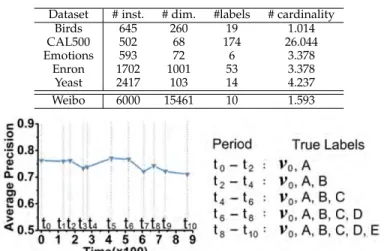
Figure 1 shows an example simulation of a data stream using the Yeast dataset, where 5 new labels (A to E) are observed in different time periods. At t0, only the initial training set with known labels (v0) is observed; and a
multi-label classifier is trained using this training set. Then, instances with possibly new label A begins to appear in the t0 −t2 period. At t1, which denotes that the buffer
7. http://mulan.sourceforge.net/datasets.html
Table 2
Characteristics of datasets used. # inst is the number of instance, # dim is the dimension, #label is the total number of class labels, and
#cardinarity is the average number of labels for each instance
Dataset # inst. # dim. #labels # cardinality
Birds 645 260 19 1.014 CAL500 502 68 174 26.044 Emotions 593 72 6 3.378 Enron 1702 1001 53 3.378 Yeast 2417 103 14 4.237 Weibo 6000 15461 10 1.593
Figure 1. Performance on Yeast dataset. 5 new labels are involved. (of instances having detected with the new label) is full, MuENLupdates the multi-label classifier ([ht,1,· · ·, ht,ℓ]) for
the expanded known label set{v0, A}; and also updates the detector (Dt) so that it can detect the next new label.
The updated classifier and detector are then used for prediction att1+ 1, which is the time that A becomes part of the known labels. At t2, new label B begins to appear, and the same process in the t0−t2 period repeats in the t2−t4 period; and the subsequent periods up to t8−t10
for label E. The classifier and detector used for prediction in each period are summarized in Table 3. Note that for detection, we always use MuENLForest; for prediction, when the classifier has not been built for the new label, we use the output of the detector MuENLForest as the prediction result; after MNLhas been updated for the new label, we useMNLfor prediction.
It is interesting to note that the overall predictive per-formance does not degenerate much with the successive appearance of new labels, as shown in Figure 1, after about 900 time steps with 5 consecutive new labels.
Table 3
Models used for predicting new labels in the simulated time periods.
Time Model for predicting new labels True labels
t0−t1 MuENLForest v0, A t1−t2 MNL v0, A t2−t3 MuENLForest v0, A, B t3−t4 MNL v0, A, B t4−t5 MuENLForest v0, A, B, C t5−t6 MNL v0, A, B, C · · · · · · · · ·
For a given dataset, the above simulation is conducted as follows. The label setvin a given dataset is split into two subsets, i.e.,vN = {va1, . . . ,va5} the candidate new label
set of 5 new labels, and vK the known label set. Let PK
withvN. Note that we need to do some pre-processing of
the given dataset: (1) if two labels are highly correlated, i.e., often co-occur, they are combined by taking a union of the two labels, since it is impossible to distinguish these labels without any prior knowledge. (2) If a label is independent of other labels, i.e., seldom co-occur with other labels, it is not as a new label, since this kind of label will degenerate to a new class detection in class incremental learning, which is an easier task; (3) those moderately correlated labels (around median in the ranked list) are potential new labels. These labels sometimes co-occur with the same label and sometimes with different labels8.
We sample 90% of PK to form the initial training set
T0= (X0, Y0). Fort >0,xtis randomly selected uniformly
(without replacement) fromPK\T0and a subset ofPN
hav-ing labelvaifor time periodt2i−2−t2iwherei= 1, . . . ,5.
For evaluation, we consider a commonly applied metric for multi-label learning, i.e., Average Precision. It is the average fraction of positive labels ranked higher than a particular positive label. Let p denote the number of test instances;Ci+ andCi− be the sets of positive and negative labels, respectively, associated with instance xi. The set
of positive predicted labels which are ranked lower than label c for xi is defined as: Qˆi,c = {j | rank(xi, j) ≤
rank(xi, c), j∈Ci+}, whererank(xi, c)is the rank of labelc
in the predicted label ranking (sorted in descending order). Then, Average Precision = 1
p ∑p i=1 1 |C+ i| ∑ c∈Ci+ |Qˆ i,c| rank(xi,c).
The larger the Average Precision, the better.
The experiment is conducted based on the simulation described above. The predictive performance is measured at
t1, . . . , t6; and two kinds of evaluations are conducted: (i)vt
-evaluation: it measures the performance with the emergence of new labels in the simulation; (ii)v0-evaluation: it assesses
how well MuENLperforms on the initial label set v0 only
throughout the entire period, i.e., the performance on the emerging new labels are not assessed.
For each dataset, the average result and standard devia-tion of 10 independent runs of simuladevia-tions are reported.
The performances of two algorithms are said to have a significant difference if the difference is more than two standard errors.
6.2 Baselines
We employ two sets of baselines to compare with MuENL: (i) the state-of-the-art multi-label approaches; (ii) variants of MuENLhaving differentMuENLcomponents.
(a) State-of-the-art multi-label approaches
We compare MuENL with BR [3], CLR [7], ECC [20], PLR, LIMO [28], and GenEML [12], which are multi-label learn-ing approaches considerlearn-ing the initially known labels only. BR, CLR, and ECC are first-order, second-order and high-order multi-label learning approaches, respectively. PLRis the multi-label approach proposed in Section 3.2.1. It is a degenerated version ofMuENLwithout a detector and model update.LIMOandGenEML are the most recently proposed
8. The correlation between two labels is measured based on cosine similarity. In order to rank label correlation among labels, we use the sum of cosine similarities of pair-wise labels. A, B, C three label vectors for example, the score for A iscos (A, B) + cos (A, C).
Table 4
MuENLvariants
Approach Classifier Detector Classifier Update
MuENLSVM PLR MuENLForest SVM
MuENLIF PLR iForest MNL
MuENLOC PLR OC-SVM MNL
MuENLOR PLR MuENLForest Oracle+PLR
MuENL PLR MuENLForest MNL
approaches to handle multi-label learning:LIMOconsiders both the instance-wise and label-wise margin andGenEML is a generative model. Further details are listed as follows:
• BRtrains a linear classifier for each label independently.
• CLRtransforms the multi-label learning problem into the label ranking problem and incorporates a virtual label to separate the relevant and irrelevant labels.
• ECC is the ensemble of classifier chains. In each chain, ground truth labels are encoded into the feature space gradually; thus high order label relations are exploited.
• PLRtakes advantage of pairwise label ranking.
• LIMOmaximizes both the label-wise margin and instance-wise margin.
• GenEMLis a flexible and scalable generative model based on a latent factor model for the label matrix.
(b) Variants ofMuENL
To further validate the effectiveness of each component, we compareMuENLwith its variants.
• MuENLIF: UseiForest[16] (instead ofMuENLForest) as the detector.
• MuENLOC: UseOC-SVM[23] (instead ofMuENLForest) as the detector.
• MuENLSVM: UseMuENLForestas the detector, but use a different classifier: train a linear classifier for the new label viaSVMby using the same training set as used inMNL.
• MuENLOR: UseMuENLForestas the detector and assume that an oracle is accessible to provide the ground truth for model updates. Its performance will be the upper bound.
These variants are summarized in Table 4.
The following codes are used to implement MuENL: LIBLINEAR toolbox [5] is applied as the linear SVM; MANOPT toolbox [2] is utilized to implement the steepest descent with a line search procedure to update the multi-label classifier.kmeanswithk= 2is applied to implement the splitting criterion inMuENLTreewhich is a binary tree.
For each method under comparison, its parameters are tuned using the initial training set at t0 via 5-fold cross-validation. Then, these settings are employed for the rest of the data stream.
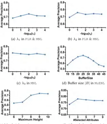
To select the appropriate settings for the detector, a label randomly selected from Y0 is used for validation, and the rest of the labels are used to train a detector. This process is repeated 5 times for a different randomly selected label in Y0 in order to choose the appropriate parameter settings for the detector. The ranges of values used are: buffer size|B| ∈ {10,15,30,60}, maximum tree heightem∈ {−2,−1,0,1}+ceil(log2ψ)(where ceil(log2ψ)
is the average height of the binary tree with sample size
ψ), number of selected attributes|q| ∈ {1,3,5}. The other parameters are fixed by default: tree number g = 100, sample sizeψ= 256andλ3= 1.
Detail ranges (or values) of the parameters ofMuENLand the baselines are summarized in Table 5.
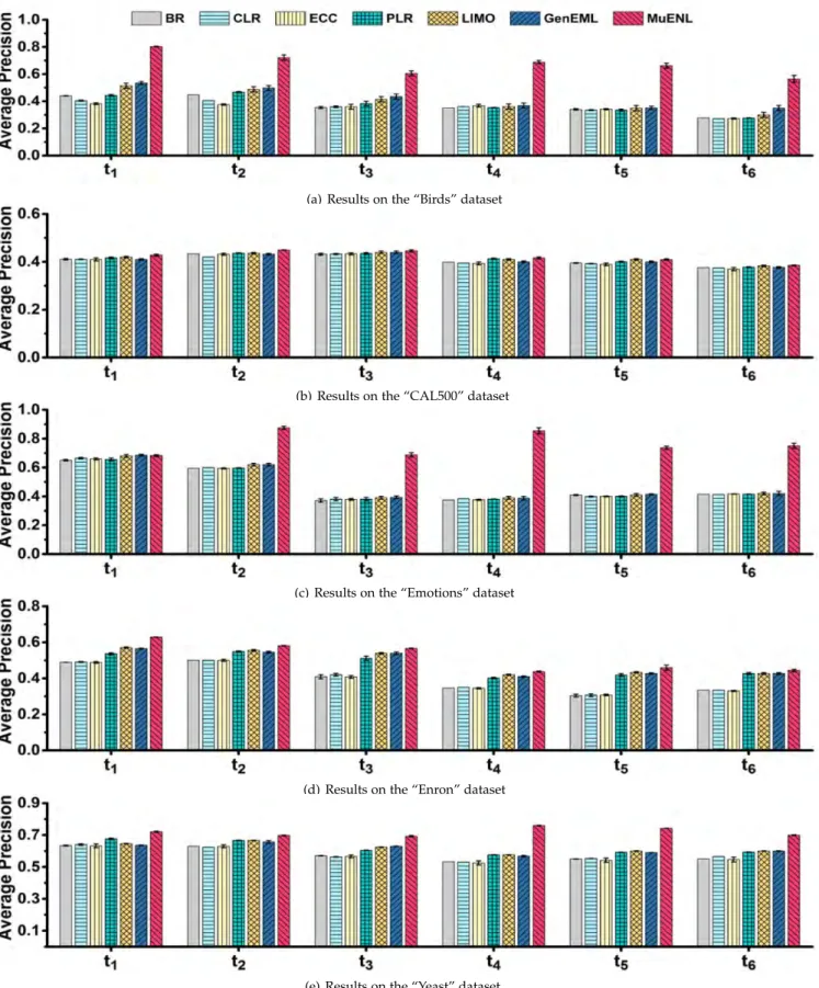
(a) Results on the “Birds” dataset
(b) Results on the “CAL500” dataset
(c) Results on the “Emotions” dataset
(d) Results on the “Enron” dataset
(e) Results on the “Yeast” dataset
Table 5
Parameters used inMuENLand its baselines
Parameter Model Approach
|B| ∈ {10,15,30,60} — MuENL MuENLvariants λ1, λ2∈ {0.001,0.01,0.1,1} PLR MuENL MuENLIF MuENLOC MuENLOR PLR&MNL |q| ∈ {1,3,5} MuENLForest g= 100 MuENL ψ= 256 MuENLSVM em∈ {6,7,8,9} λ3= 1 MNL MuENL MuENLOC MuENLIF C∈ {0.1,1,10,100} SVM MuENLSVM BR,CLR,ECC g= 100 iForest MuENLIF ψ= 256 em∈ {6,7,8,9} nu∈ {0.3,0.5,0.7} OC-SVM MuENLOC 6.3 Experimental Results
We conduct two sets of experiments which differ in the number of new labels which may appear in each time period. The first set has exactly one new label; whereas the second set has more than one new label. The second set assesses how multiple new labels in each time period may affect the predictive performance.
6.3.1 Results on one new label per time period (a) Compare with existing Multi-label approaches
Figure 1 is an example plot of vt-evaluation on the Yeast
dataset having one new label in each time period over 5 periods9. In general, MuENL maintains a good predictive performance spanning the entire duration from t0 to t10. This is a direct result of a good detector and a robust classifier inMuENL.
Figure 2 summarizes the comparison withBR,ECC,CLR, PLR,LIMO, and GenEML in terms of vt-evaluation in five
datasets. It is interesting to note thatMuENLalmost always performs better than all baselines. Many of the differences are significant.
Figure 3. Compare BR, CLR, ECC,PLR, LIMO,GenEML, andMuENL: Results usingv0-evaluation.
The summarised result on five datasets forv0-evaluation
is provided in Figure 3 in terms of average precision.MuENL achieves better or comparable performance in comparison with all baselines. This shows thatMuENL, which incorpo-rates detection and prediction of new labels, not only does
9. Notice that the time when the buffer gets full may be different in different time periods, and for different detectors in the same time period. Thus, the duration of one period may vary from one period to another and from one detector to another.
Figure 4. CompareMuENLvariants: Results usingvt-evaluation.
Figure 5. Detection performance of MuENLForest, OC-SVM and
iForest(i.e., detectors in threeMuENLvariants) att1.
no harm to the performance on known labels, but can also gain better performance because pairwise label ranking is considered.
(b) Compare withMuENLvariants
Figure 4 presents the result based on average precision. Among the four MuENLvariants,MuENLORhas the best performance since it uses the oracle which provides the ground truth that is not available to the other variants. Note that this oracle is available in practice and it is used to show the upper bound.
MuENLobtains a performance comparable withMuENLOR in all cases, where there is no significant difference in performance. This is a direct result of a good detector and a robust classifier for both known and new labels.
MuENLachieves a significantly better performance than MuENLSVMon all datasets. This shows that the robust clas-sifier update procedure inMuENLworks better than that in SVM; and it is essential in maintaining a good performance in a dynamic learning environment.
MuENLIF and MuENLOC replace the detector in MuENL with iForest and OC-SVM, respectively. Even though a robust update procedure is applied in both of them,MuENL still performs better than them (on 4 of 5 datasets,MuENL is significantly better). This validates the effectiveness of the detector inMuENL. Because new labels often co-occur with known labels, this kind of occurrences confuses existing detectors OC-SVM or iForest—leading to low detection accuracy. By taking both the feature and label information into account,MuENLForestis able to differentiate instances with a combination of features and label patterns due to new labels from that due to existing labels. This yields a better detection outcome as a result.
A more direct analysis of the above comparison is pro-vided in Figure 5 which shows detection performance of MuENLForest,OC-SVM and iForestin terms of the F1-score evaluated at t1. As expected, MuENLForest outper-forms the other competitors.
For the classifier of new labels, we make a more direct comparison of the proposedMNLwithSVMandPLRwhich treat the instances in the buffer as positive ones and other
Figure 6. Classifier performance ofMNL,SVMandPLR(i.e., classifiers in threeMuENLvariants) att2.
seen instances as negative ones in order to train a classifier. Figure 6 shows the performance evaluated at t2 (In this
experiment, the same detector MuENLForest is applied). Figure 6 shows thatMNLis better thanSVMandPLRbecause it employs a robust update, which works well even under the condition that a detector is imperfect.
To examine the significance of the relative performance among these algorithms, we perform a post-hoc Nemenyi test [10]. The result shown in Figure 7 reveals that the pro-posedMuENLis significantly better than all the traditional multi-label approaches (which do not consider any new labels) and otherMuENLvariants, exceptMuENLORin which the oracle is available.
Figure 7. Critical difference (CD) diagram of the post-hoc Nemenyi test (α= 0.05) for the comparison results with both the traditional multi-label learning approaches andMuENLvariants. The difference between two algorithms is significant if the gap between their ranks is larger than the CD. There is a line between two algorithms if the rank gap between them is smaller than the CD.
(c) Compare withLP-SENCForest
SENCForest[19] is proposed recently to handle class in-cremental learning on streaming data, and has achieved a success. It provides a unified tree-based model for new class detection and known class prediction.SENCForestfocuses on a multi-class setting—each instance belongs to a single class only. To applySENCForest in the multi-label learn-ing settlearn-ing, we first applyLabel Powerset (LP)[25] to encode different label combinations as different classes to transform multi-label learning into multi-class setting, be-foreSENCForestis applied. We name itLP-SENCForest, which is the counterpart ofSENCForestin our setting.
Figure 8 summarizes the comparison results of av-eraged performance on the whole data stream in five datasets. As can be observed, MuENL is much better than LP-SENCForest. This result is not surprising because: (1) LPtransformation leads to too many classes, some of them hold a small number of instances.SENCForestdoes poorly because it requires a sufficient number of instances for each class in order to do well. (2) AfterLPtransformation, the
de-Figure 8.MuENLversusLP-SENCForest
tected new class bySENCForestcan be a new combination of existing labels, but does not contain any new labels. (d) Results with different label sequences
In order to further validate the effectiveness of our ap-proach, the evaluation is conducted multiple trials on a dataset, where each trial has a different random order of known and new labels on the simulated stream. The com-parison is done with two best performing methods in each of two approaches, i.e., the multi-label approach:PLRand LIMO10, and twoMuENLvariants:MuENLOCandMuENLIF.
We report the averaged difference from the baselineBR in MicroF1, which is a label based measure: MicroF1 =
2∑i,jyi,jhi,j
∑
i,jyi,j+∑i,jhi,j, i ∈ {1,· · ·, T}, j ∈ {1,· · ·,|vt|}, on the
entire data stream as in Figure 9. The result that MuENL outperforms these four methods, even under random orders of new labels.
Figure 9. CompareBR,PLR,LIMO,MuENLOC,MuENLIFwith different
label sequences as new labels: Results using the difference in MicroF1 fromBR.
6.3.2 Results on multiple new labels per time period When more than one new label occurs in a time period, MuENLcan also be used by treating these new labels as a single meta label. Specifically, if any instance has a subset of labels, encapsulated by a meta-label, then the instance has this meta-label. The goal in this setting is to detect and classify a new meta label, if it exists, in each time period.
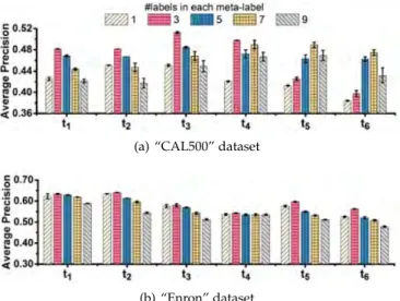
We conduct experiments, where the number of new labels varies from 1 to 9 in each time period, to examine the effect of multiple labels in comparison with the baseline which has only one new label per time period. The evalua-tion is based on the meta label we specified at the beginning of the data stream.
Figure 10 shows that results in two datasets. Both results show that the MuENL approach can handle multiple new labels; and in many cases, it performs better in the multiple-new-labels scenarios than in the single-new-label scenarios. This is because the learning task for a meta label of multiple
(a) “CAL500” dataset
(b) “Enron” dataset
Figure 10.MuENL’s performance in scenarios having different numbers of new labels in each time period
labels can be easier than that for a single label, depending on the data distribution. An example is shown Figure 10(a).
7
EXPERIMENTS ON HIGH DIMENSIONAL DATA
7.1 DatasetWe have collected a total of 6,000 Weibo instances in 10 topics: traffic, car, president, Nobel prize, TV show, music, video, advertisement, sports, finance (indexed as 1 - 10). We extracted the bag-of-words features which resulted in 15,461 features. As a consequence, the data is very sparse, i.e., only 0.2%of the total number of features have non-zero values; and each instance belongs to 1.61 labels on average.
When it begins att0, there are only 5 known labels, and the rest of them will successively emerge as new labels. Five new labels emerge successively at different times, denoted ast1, t2,· · ·, t5. On average, the interval between the sub-sequent emergence of two new labels has 1,000 instances. For experiments, we permute the order of class labels, and conduct 5 runs to avoid the influence of new label order on the results.
7.2 Baselines
We compareMuENLHDwith two baselines:
• MuENL: Directly apply MuENL on the high dimensional sparse data stream.
• MuENL+PCA: First, we perform PCA on the observed data at time t0 to obtain the mapping from the original space to a low dimensional subspace (whered′= 100). Then, we transform each arriving instance to the low dimensional representation via this mapping. We apply MuENLon the transformed data.
• MuENL+MultiPCA: Unlike MuENL+PCA, which performs PCA only at t0,MuENL+MultiPCAapplies PCA multiple
times, i.e., a new PCA is conducted on a data chunk collected during the period in-between the buffer is empty and full.
The parameter setting of MuENL is the same as that used in Section 6. The settings for MuENLHD are given as follows: the number of the random featuresm= 2000, and the number of attributes in the transformed space is set as
d′= 100.
Table 6
Total time used to handle the data stream with 6,000 instances.
MuENL MuENL+PCA MuENL+MultiPCA MuENLHD
Time (s) 120,839 507 1417 1,442
7.3 Experimental results
We evaluate the performance in terms of Average Precision on 100 instances at every time point oft0, t1,· · ·,t5. The performances ofMuENLHD,MuENL+PCA,MuENL+MultiPCA areMuENLare exhibited in Figure 11. As expected, all algo-rithms have comparable performance at timet0. However, MuENLHDachieves much better performance than the other contenders at t1 to t5. This is mainly due to fact that streaming kernel PCA captures the main information of the data stream in different time periods; and those transformed low dimensional representations work well collaboratively with the predictive information from the classifiers.
Although MuENL+PCA reduces the dimensionality to the same as that of MuENLHD, it performs worse because MuENL+PCAonly trains PCA att0, and keeps the linear map-ping throughout the stream. This strategy leads to a worse performance in the following detection, since emerging new instances are not considered. In contrast.MuENLHD adapts the dimension reduction throughout the stream.
For MuENL+MultiPCA, PCA is applied each time the MuENL’s models are updated for an emerging new label. Even though PCA has been applied multiple times to adapt to the data stream, only the latest data chunk is considered. In contrast,MuENLHDadapts along the stream. As a result, MuENLHDoutperformsMuENL+MultiPCA.
Figure 11. Compare MuENL+PCA, MuENL+MultiPCAand MuENLHD: Result shown is the difference from MuENL in terms of Average Pre-cision at each time point.
We also make a comparison on the time spent to handle the whole stream, shown in Table 6. As can be observed, MuENL takes nearly 100 times longer than MuENLHD to handle the high dimensional data stream. This is consistent with the factor of reduction from 15000 to 100 dimen-sions. ThoughMuENL+PCAis 3 times faster thanMuENLHD, they are in the same order. MuENLHD needs the extra time in order to update the nonlinear mapping through-out the stream. MuENLHD has about the same run time as MuENL+MultiPCA, but it achieves much better perfor-mance.
8
THE EFFECT OF PARAMETERS
We study the effect of parameters in this section. The ex-periment is conducted in one run, where settings of the parameters are determined via 5-fold cross-validation before