University of Central Florida University of Central Florida
STARS
STARS
Electronic Theses and Dissertations, 2004-2019
2016
a priori synthetic sampling for increasing classification sensitivity
a priori synthetic sampling for increasing classification sensitivity
in imbalanced data sets
in imbalanced data sets
William Rivera
University of Central Florida
Part of the Engineering Commons
Find similar works at: https://stars.library.ucf.edu/etd
University of Central Florida Libraries http://library.ucf.edu
This Doctoral Dissertation (Open Access) is brought to you for free and open access by STARS. It has been accepted for inclusion in Electronic Theses and Dissertations, 2004-2019 by an authorized administrator of STARS. For more information, please contact [email protected].
STARS Citation STARS Citation
Rivera, William, "a priori synthetic sampling for increasing classification sensitivity in imbalanced data sets" (2016). Electronic Theses and Dissertations, 2004-2019. 4895.
A PRIORI SYNTHETIC SAMPLING FOR INCREASING CLASSIFICATION SENSITIVITY IN IMBALANCED DATA SETS
by
WILLIAM A. RIVERA B.S. DeVry University, 2012 M.S. University of West Florida, 2013 M.S. University of Central Florida, 2015
A dissertation submitted in partial fulfilment of the requirements for the degree of Doctor of Philosophy
in the College of Engineering and Computer Science at the University of Central Florida
Orlando, Florida
Spring Term 2016
c
ABSTRACT
Building accurate classifiers for predicting group membership is made difficult when data is skewed or imbalanced which is typical of real world data sets. The classifier has the tendency to be biased towards the over represented group as a result. This imbalance is considered a class imbalance problem which will induce bias into the classifier particularly when the imbalance is high.
Class imbalance data usually suffers from data intrinsic properties beyond that of imbalance alone. The problem is intensified with larger levels of imbalance most commonly found in observational studies. Extreme cases of class imbalance are commonly found in many domains including fraud detection, mammography of cancer and post term births. These rare events are usually the most costly or have the highest level of risk associated with them and are therefore of most interest.
To combat class imbalance the machine learning community has relied upon embedded, data pre-processing and ensemble learning approaches. Exploratory research has linked several factors that perpetuate the issue of misclassification in class imbalanced data. However, there remains a lack of understanding between the relationship of the learner and imbalanced data among the compet-ing approaches. The current landscape of data preprocesscompet-ing approaches have appeal due to the ability to divide the problem space in two which allows for simpler models. However, most of these approaches have little theoretical bases although in some cases there is empirical evidence supporting the improvement.
The main goals of this research is to introduce newly proposed a priori based re-sampling methods that improve concept learning within class imbalanced data. The results in this work highlight the robustness of these techniques performance within publicly available data sets from different domains containing various levels of imbalance. In this research the theoretical and empirical
TABLE OF CONTENTS
LIST OF FIGURES . . . x
LIST OF TABLES . . . xii
CHAPTER 1: INTRODUCTION . . . 1
Background . . . 1
Motivation . . . 3
Current Approaches to Combat Class Imbalance . . . 6
Research Gaps . . . 7
Research Questions . . . 8
Research Limitations . . . 9
Dissertation Overview . . . 10
CHAPTER 2: LITERATURE REVIEW . . . 12
Data Intrinsic Properties of Imbalanced Data . . . 13
Disjunction . . . 15
Class Overlap . . . 17
Noisy Data . . . 18
Data Set Shift . . . 19
Standard Classification Algorithms . . . 19
Prediction Estimation . . . 20
Least Square Estimation Approach . . . 21
Maximum Likelihood Estimation Approach . . . 22
Fisher’s Linear Discriminate Analysis . . . 24
Logistic Regression . . . 27
Support Vector Machine . . . 30
Artificial Neural Network . . . 33
Techniques for Dealing with Imbalanced Data . . . 35
Embedded Approaches . . . 35
Active Learning . . . 36
Kernel Based methods . . . 37
Cost Assignment Approaches . . . 38
Feature Selection . . . 41
Re-sampling . . . 42
Over-Sampling . . . 42
Random (ROS) and Focused Re-Sampling . . . 43
Synthetic Oversampling Minority Technique (SMOTE) . . . . 44
Borderline-SMOTE . . . 45
Safe-Level-SMOTE . . . 46
Local Neighbourhood Extension to SMOTE (LN-SMOTE) . . 47
Adaptive Synthetic (ADASYN) Sampling Approach . . . 47
Under-Sampling . . . 49
Propensity Score Matching (PSM) . . . 49
Random (RUS) and Cluster Based Under-Sampling . . . 51
Tomek Links (TK) Re-Sampling . . . 51
Condensed Nearest Neighborhood (CNN) Re-Sampling . . . . 52
One Sided Selection . . . 52
Edited Nearest Neighborhood (ENN) and Neighborhood Clean-ing Rule (NCR) Re-SamplClean-ing . . . 53
Evaluation Metrics for Imbalanced Data . . . 57 Sensitivity . . . 59 Specificity . . . 59 Precision . . . 60 F Measure . . . 60 G Mean . . . 61
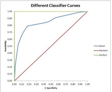
ROC Curves and AUC Measures . . . 61
Summary . . . 63
CHAPTER 3: RESEARCH METHODS . . . 65
A Priori Synthetic Sampling . . . 65
Over-Sampling using Propensity Scores (OUPS) . . . 65
Stopping Conditions . . . 67
Benefits of OUPS . . . 68
Safe Level OUPS . . . 69
Experimental Data Sets . . . 73
Algorithm Selection . . . 76
Experimental Description . . . 78
Techniques for Comparison . . . 79
Statistical Tests . . . 80
CHAPTER 4: RESULTS . . . 81
Experimental Results . . . 81
Over-Sampling Results . . . 82
Results By Learner . . . 84
Results Per Imbalance Level . . . 89
Results by Increasing Stopping Threshold . . . 95
Results of Mixing Under and Over-Sampling . . . 97
Results by Learner . . . 100
SVM with an RBF Kernel . . . 100
SVM with a Linear Kernel . . . 103
LDA . . . 106
Logistic Regression . . . 109
Neural Networks . . . 112
Simulated Samples and SVM . . . 116
Visual Representation . . . 118
CHAPTER 5: CONCLUSION . . . 122
Recommendations . . . 124
Limitations . . . 126
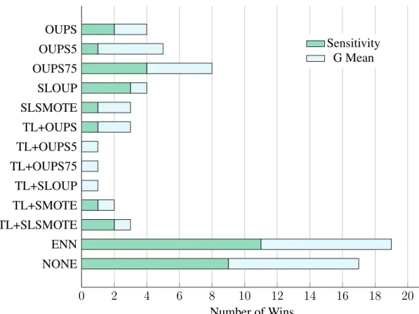
APPENDIX A: WINS BY TECHNIQUE NEMENYI TEST . . . 128
APPENDIX B: SVM RBF STATISTICAL TESTS (HOLM METHOD) . . . 137
APPENDIX C: SVM LINEAR STATISTICAL TESTS (HOLM METHOD) . . . 150
APPENDIX D: LDA STATISTICAL TESTS (HOLM METHOD) . . . 163
APPENDIX E: LOGISTIC REGRESSION STATISTICAL TESTS (HOLM METHOD) . . 176
APPENDIX F: NEURAL NETWORKS STATISTICAL TESTS (HOLM METHOD) . . . 189
APPENDIX G: OVERSAMPLING COMPARISONS STATISTIAL TESTS . . . 202
LIST OF FIGURES
Figure 1.1: Supervised Learning Process . . . 2
Figure 1.2: Spectrum of the Imbalance Problem Space . . . 3
Figure 2.1: Class Imbalance Data . . . 13
Figure 2.2: Example of Small Disjuntcs in Data . . . 15
Figure 2.3: Example of Class Overlap and Borderline Observations in Data . . . 18
Figure 2.4: Support Vector Machine [15] . . . 30
Figure 2.5: Artificial Neural Network . . . 34
Figure 2.6: Taxonomy of Embedded Techniques . . . 40
Figure 2.7: Taxonomy of Resampling Techniques . . . 54
Figure 2.8: Taxonomy of Ensemble Techniques [63] . . . 57
Figure 2.9: Example of ROC Curve Plot . . . 62
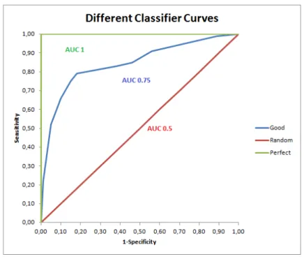
Figure 2.10:Example of AUC Calculated From the ROC Curve Plot . . . 63
Figure 4.1: OUPS75 Number of Wins (Sensitivity) Neural Networks 5,10 20 . . . 86
Figure 4.2: Extreme Imbalance - Number of Wins by Sample Technique . . . 92
Figure 4.4: Medium Imbalance - Number of Wins by Sample Technique . . . 94
Figure 4.5: Low Imbalance - Number of Wins by Sample Technique . . . 94
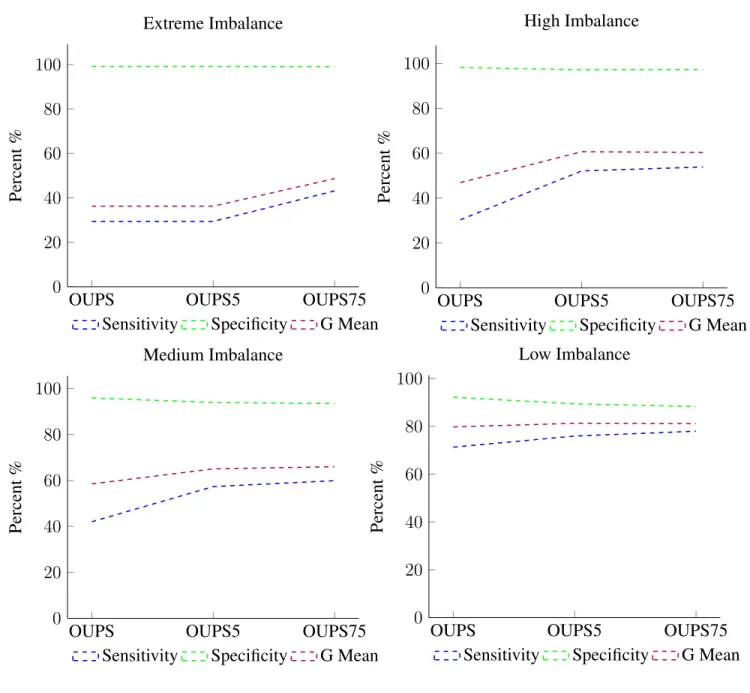
Figure 4.6: OUPS Performance by Increase in Threshold . . . 96
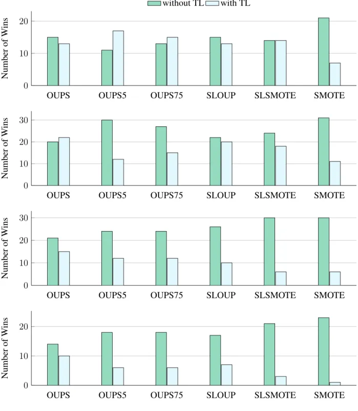
Figure 4.7: TL Under-Sampling Versus no Under-Sampling - Win Ratio for Sensitivity. Extreme,High, Medium and Low Imbalance from Top to Bottom . . . 98
Figure 4.8: TL Under-Sampling versus no Under-Sampling - Win Ratio for G Mean. Extreme, High, Medium and Low Imbalance from Top to Bottom . . . 99
Figure 4.9: Random Sample . . . 119
Figure 4.10:After Applying Safe Level OUPS . . . 120
LIST OF TABLES
Table 1.1: Cost Benefit Matrix . . . 4
Table 1.2: Imbalance Levels . . . 10
Table 2.1: Cost Matrix . . . 38
Table 2.2: Region Definitions [43, 14] . . . 45
Table 2.3: Confusion Matrix . . . 58
Table 3.1: Region Definitions [43, 14] . . . 70
Table 3.2: Data Summary . . . 74
Table 3.3: Data Summary Continued . . . 75
Table 3.4: Confusion Matrix . . . 77
Table 4.1: Imbalance Levels . . . 82
Table 4.2: Overall Results . . . 83
Table 4.3: Top Performers Ranked By Learner for G Mean . . . 85
Table 4.4: Probablistic Learners (LDA,Logistic Regression) . . . 87
Table 4.5: Results using NN with 5,10 and 20 Nodes . . . 88
Table 4.7: Experimental Data . . . 90
Table 4.8: Extreme Imbalance (Left) and High Imbalance(Right) using RBF SVM . . . 102
Table 4.9: Medium Imbalance (Left) and Low Imbalance (Right) using RBF SVM . . . 103
Table 4.10:Extreme Imbalance (Left) and High Imbalance(Right) using Linear SVM . . 105
Table 4.11:Medium Imbalance (Left) and Low Imbalance (Right) using Linear SVM . . 106
Table 4.12:Extreme Imbalance(Left) and High Imbalance (Right) using LDA . . . 108
Table 4.13:Medium Imbalance(Left) and Low Imbalance (Right) using LDA . . . 109
Table 4.14:Extreme Imbalance(Left) and High Imbalance (Right) using Logstic Regression111 Table 4.15:Medium Imbalance(Left) and Low Imbalance (Right) using Logstic Regression112 Table 4.16:Extreme Imbalance(Left) and High Imbalance (Right) using Neural Networks 114 Table 4.17:Medium Imbalance(Left) and Low Imbalance (Right) using Neural Networks 115 Table 4.18:SVM using Simulated Data . . . 117
Table 4.19:Paired T TestpValues - Sensitivity (Left) Specificity (Middle) G Mean (Right)117 Table 5.1: Recommended Technique . . . 126
Table A.1: Extreme Imbalance Sensitivity Nemenyi TestpValues . . . 129
Table A.2: Extreme Imbalance G Mean Nemenyi TestpValues . . . 130
Table A.4: High Imbalance G Mean Nemenyi TestpValues . . . 132
Table A.5: Medium Imbalance Sensitivity Nemenyi TestpValues . . . 133
Table A.6: Medium Imbalance G Mean Nemenyi TestpValues . . . 134
Table A.7: Low Imbalance Sensitivity Nemenyi TestpValues . . . 135
Table A.8: Low Imbalance G Mean Nemenyi TestpValues . . . 136
Table B.1: Extreme Imbalance SensitivitypValues (Holm Method) . . . 138
Table B.2: Extreme Imbalance SpecificitypValues (Holm Method) . . . 139
Table B.3: Extreme Imbalance G MeanpValues (Holm Method) . . . 140
Table B.4: High Imbalance SensitivitypValues (Holm Method) . . . 141
Table B.5: High Imbalance SpecificitypValues (Holm Method) . . . 142
Table B.6: High Imbalance G MeanpValues (Holm Method) . . . 143
Table B.7: Medium Imbalance SensitivitypValues (Holm Method) . . . 144
Table B.8: Medium Imbalance SpecificitypValues (Holm Method) . . . 145
Table B.9: Medium Imbalance G MeanpValues (Holm Method) . . . 146
Table B.10:Low Imbalance SensitivitypValues (Holm Method) . . . 147
Table B.11:Low Imbalance SpecificitypValues (Holm Method) . . . 148
Table C.1: Extreme Imbalance SensitivitypValues (Holm Method) . . . 151
Table C.2: Extreme Imbalance SpecificitypValues (Holm Method) . . . 152
Table C.3: Extreme Imbalance G MeanpValues (Holm Method) . . . 153
Table C.4: High Imbalance SensitivitypValues (Holm Method) . . . 154
Table C.5: High Imbalance SpecificitypValues (Holm Method) . . . 155
Table C.6: High Imbalance G MeanpValues (Holm Method) . . . 156
Table C.7: Medium Imbalance SensitivitypValues (Holm Method) . . . 157
Table C.8: Medium Imbalance SpecificitypValues (Holm Method) . . . 158
Table C.9: Medium Imbalance G MeanpValues (Holm Method) . . . 159
Table C.10:Low Imbalance SensitivitypValues (Holm Method) . . . 160
Table C.11:Low Imbalance SpecificitypValues (Holm Method) . . . 161
Table C.12:Low Imbalance G MeanpValues (Holm Method) . . . 162
Table D.1: Extreme Imbalance SensitivitypValues (Holm Method) . . . 164
Table D.3: Extreme Imbalance G MeanpValues (Holm Method) . . . 165
Table D.4: High Imbalance SensitivitypValues (Holm Method) . . . 166
Table D.5: High Imbalance SpecificitypValues (Holm Method) . . . 167
Table D.7: Medium Imbalance SensitivitypValues (Holm Method) . . . 169
Table D.8: Medium Imbalance SpecificitypValues (Holm Method) . . . 170
Table D.9: Medium Imbalance G MeanpValues (Holm Method) . . . 171
Table D.10:Low Imbalance SensitivitypValues (Holm Method) . . . 172
Table D.11:Low Imbalance SpecificitypValues (Holm Method) . . . 173
Table D.12:Low Imbalance G MeanpValues (Holm Method) . . . 174
Table D.2: Extreme Imbalance SpecificitypValues (Holm Method) . . . 175
Table E.1: Extreme Imbalance SensitivitypValues (Holm Method) . . . 177
Table E.2: Extreme Imbalance SpecificitypValues (Holm Method) . . . 178
Table E.3: Extreme Imbalance G MeanpValues (Holm Method) . . . 179
Table E.4: High Imbalance SensitivitypValues (Holm Method) . . . 180
Table E.5: High Imbalance SpecificitypValues (Holm Method) . . . 181
Table E.6: High Imbalance G MeanpValues (Holm Method) . . . 182
Table E.7: Medium Imbalance SensitivitypValues (Holm Method) . . . 183
Table E.8: Medium Imbalance SpecificitypValues (Holm Method) . . . 184
Table E.9: Medium Imbalance G MeanpValues (Holm Method) . . . 185
Table E.11:Low Imbalance SpecificitypValues (Holm Method) . . . 187
Table E.12:Low Imbalance G MeanpValues (Holm Method) . . . 188
Table F.1: Extreme Imbalance SensitivitypValues (Holm Method) . . . 190
Table F.2: Extreme Imbalance SpecificitypValues (Holm Method) . . . 191
Table F.3: Extreme Imbalance G MeanpValues (Holm Method) . . . 192
Table F.4: High Imbalance SensitivitypValues (Holm Method) . . . 193
Table F.5: High Imbalance SpecificitypValues (Holm Method) . . . 194
Table F.6: High Imbalance G MeanpValues (Holm Method) . . . 195
Table F.7: Medium Imbalance SensitivitypValues (Holm Method) . . . 196
Table F.8: Medium Imbalance SpecificitypValues (Holm Method) . . . 197
Table F.9: Medium Imbalance G MeanpValues (Holm Method) . . . 198
Table F.10: Low Imbalance SensitivitypValues (Holm Method) . . . 199
Table F.11: Low Imbalance SpecificitypValues (Holm Method) . . . 200
Table F.12: Low Imbalance G MeanpValues (Holm Method) . . . 201
Table G.1: Overall Results Sensitivity Statistical TestpValues (Holm Method) . . . 203
Table G.2: Overall Results Specificity Statistical TestpValues (Holm Method) . . . 204
Table G.4: Probablistic Learners Sensitivity Statistical TestpValues (Holm Method) . . 206
Table G.5: Probablistic Learners Specificity Statistical TestpValues (Holm Method) . . 207
Table G.6: Probablistic Learners G Mean Statistical TestpValues (Holm Method) . . . . 208
Table G.7: Neural Networks Sensitivity Statistical TestpValues (Holm Method) . . . 209
Table G.8: Neural Networks Specificity Statistical TestpValues (Holm Method) . . . 210
Table G.9: Neural Networks G Mean Statistical TestpValues (Holm Method) . . . 211
Table G.10:SVM Sensitivity TestpValues (Holm Method) . . . 212
Table G.11:SVM Specificity TestpValues (Holm Method) . . . 213
CHAPTER 1: INTRODUCTION
Background
The task of prediction has become synonymous with the term machine learning. The field of machine learning is a branch of artificial intelligence and sub-field of computer science which attempts to have computers learn from data. Since most of the algorithms produced by machine learning communities attempt to predict choices and decisions the term has evolved to take on a much broader meaning as the study of predictive algorithms that learn from data.
The main objective for machine learning is to learn from data to predict the outcomes on new data as deemed most like what has been observed in the past. This includes clustering like items, defining rules or determining decision boundaries based on an observed data set. Successful appli-cations of learning systems have include disciplines such as medical diagnosis, natural language processing, image and speech recognition, robotics, music and mathematics [17, 11, 44, 72]
Two common approaches used to train systems include unsupervised and supervised learning tech-niques [44, 49]. In supervised learning (figure 1.1) data is partitioned into at least two subsets. One set is used as a training set to develop a model learned from the training data. The remaining set is the test set used to evaluate the model. The predicted value from the test set is compared against the known outcomes to validate its performance. This provides a mechanism to see how well the model can predict against unseen data provided there are no fundamental differences. Selecting additional subsets can also be used for refining model variables and cross validating parameter choices within algorithms.
Figure 1.1: Supervised Learning Process
One of the more common supervised learning tasks includes prediction of group membership which is also called classification. In two group or binary classification the predicted outcome of interest is limited to two discrete groups namely y ∈ {G0, G1}. The task of accurately
pre-dicting group membership is often difficult when dealing with large data sets that have a disparity between the two groups. This imbalance is considered a class imbalance problem and it is com-mon for real world data to have a degree of imbalance. Class imbalance is usually associated with extremely skewed data although technically any disparity can be considered imbalance.
The most noticeable issue with class imbalance is that the learner or classifier tends to be biased towards the over represented or majority group. Since the performance for prediction is based on the number of correctly identified samples the performance metric may remain high although the target of interest is group membership in the under represented or minority group. Exploratory research has linked several factors that perpetuate the issue of misclassification in class imbalanced data. However, there remains a lack of understanding between the relationship of the learner
and imbalanced data among competing approaches. The current landscape of data preprocessing approaches have appeal due to the ability to divide the problem space by first perturbing the original data which allows secondly for building simpler models. However, most of these approaches have little theoretical bases although in some cases there is empirical evidence supporting the improvement.
Motivation
Classification problems typically fall into 4 categories ranging from full balance to one group classification. In a two group scenario each group has members with similar characteristics ranging in size from extreme imbalance ratios to full balance. When the ratio is really low and non members of the majority group do not share characteristics the problem becomes an anomaly detection problem which is different from class imbalance. Figure 1 depicts the spectrum of these ranges.
0% One−Class each−unique AnomalyDetection (0−50%) Imbalance 50% F ullBalance
Figure 1.2: Spectrum of the Imbalance Problem Space
To have a better understanding of the issue with class imbalance lets consider an example based on a real world scenario involving fraud detection within a known class of fraud transactions. Assume that our goal is to predict members of the fraud group. Observing past data provides evidence that the disparity between groups has been observed to be as much as 100 to 1. Constructing a classifier for prediction with a 99% accuracy is trivial if we simply classify all cases as
non-early detection nor saving associated costs.
We can construct a cost benefit matrix outlining the different scenarios as shown in table 1.1. Predicting an actual fraud case that is fraud can help savexdollars while predicting fraud occurred when it did not results in money spent to investigate the case which we assume is<< x. We can say the cost is a fraction of what you would otherwise gain, xy. Correctly identifying non-fraudulent cases give us no benefit while predicting non-fraud when fraud does occurs result in an expense or cost ofx.
Table 1.1: Cost Benefit Matrix
Prediction Yes No Fraud Yes +x -x No −x y 0
The optimal scenario would be if we can correctly identify each case but that may not be feasible so an alternative scenario is to increase the ability to identify cases which are actually fraud and reduce those which are not fraud but are predicted to be. In a similar fashion to the cost benefit matrix a confusion matrix can be constructed to provide the results of classification where each cell corresponds to the amount that fell into that category. For example the cell with a benefit of+x
would correspond to the true positives, the cell with a cost of−x corresponds to false negatives, the cell with a cost of−x
negatives. The expected values can be calculated in the discrete case as: E(X, Y) = X i X j p{xi, yj} ·xiyj = X i X j p{yj} ·p{xi|yj} ·xiyj (1.1)
wherei, j corresponds to theith row andjthcell in the cost benefit matrix. In this case we can produce the following expected value:
E(prediction, f raud) = (p{f raud =yes} ·p{predicted=yes|f raud =yes} ·x)
+(p{f raud=yes} ·p{predicted=no|f raud =yes} · −x)
+(p{f raud=no} ·p{predicted=yes|f raud =no} · −x y) +(p{f raud=no} ·p{predicted=no|f raud =no} ·0)
(1.2)
Using the 99% accuracy scenario where we automatically classify all examples as not fraud we incur a cost of xn where n is the number of fraudulent transactions that do actually occur. In general the under represented examples (p{f raud = yes}) provide the most benefit or cost. Identifying just half correctly reduces the benefit/cost to 0 because xn2 −xn2 = 0. In general increasing the benefit x depends on the accuracy of the classifier for detecting fraud cases, if
p{predicted=yes|f raud=yes}> p{predicted=no|f raud=yes}then the ability to predict the target group correctly minimizes the cost spent and maximizes the costs saved. Thus the need to properly identify the under represented group is worth studying.
Current Approaches to Combat Class Imbalance
To combat class imbalance the machine learning community has relied upon three broad ap-proaches which are discussed in detail in chapter 2 and briefly mentioned here. They are em-bedded [45, 100, 27, 60], data preprocessing [101, 41, 29, 19, 47, 90, 39] and ensemble learning [88, 91, 52, 90] approaches. All of these techniques are useful when collecting data is expensive or difficult.
Embedded approaches attempt to change the internal properties of the learner to compensate for the class imbalance. This includes the addition of loss or cost functions that attempt to re-weight both majority and minority group observations, kernel based methods which apply kernel adjustment techniques or the use of active learning.
Data preprocessing approaches attempt to preprocess the data before using a learner in order to divide the problem space in two. These are also considered external since they occur externally of the learner while embedded approaches occur internally. Typical preprocessing steps include feature selection and re-sampling strategies comprised of both over and under-sampling.
Common over-sampling strategies have included focused re-sampling, random over-sampling (ROS), adaptive synthetic (ADASYN) sampling and Synthetic Oversampling Minority Technique (SMOTE). The most commonly researched approach for over-sampling is arguable SMOTE. Although SMOTE has been combined with other techniques to improve class imbalance classification there is very little research in competing approaches that use more than just the distance measures between features alone. [43, 14, 65, 29, 47, 65, 70, 82, 92].
Under-sampling approaches have been empirically shown to greatly increase accuracy compared to over-sampling or even a combination of over and under-sampling. However, the fundamental and theoretical reasons why have not been fully explored or explained [99]. Common under-sampling
techniques include random under-sampling (RUS), one sided selection (OSS), tomek links (TK), condensed nearest neighborhood (CNN), edited nearest neighborhood (ENN) and neighborhood cleaning rule (NCR).
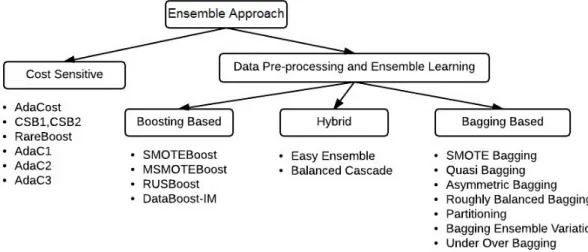
The last group of approaches are ensemble learning techniques which implement a collection of models and chooses the best approach which may include an aggregation of the best approaches. Techniques such as bagging, random forest and boosting allow for ensembles to be individually generated and weighted against other ensembles based on performance. Ensembles have become exceedingly popular for dealing with class imbalance partly because they offer the ability for both data preprocessing and embedded modification combinations.
It is important to mention that all of these above mentioned techniques represent baseline tech-niques that have been extensively researched, combined and extended allowing for incremental increases in performance.
Research Gaps
Over-sampling techniques have not been fully explored and current over-sampling approaches are limited to either random sampling or to just some combination involving the SMOTE method. Additionally, the techniques that do perform synthetically generated over-sampling as opposed to duplicate samples are based on some modification to the SMOTE method. These techniques usually rely solely on selecting somek nearest neighbor (knn) using the euclidean distance met-ric which is often problematic for dealing with high dimensional data. In most of the empimet-rical studies reviewed there was not many that studied other commonly known distance metrics such as Manhattan, Euclidean squared, Minkowski or Mahalanobis although it is trivial to consider.
imbal-ance data have not successfully linked the data intrinsic problems that contribute to poor learning performance with class imbalance data although they have been shown to empirically increase per-formance. In general over-sampling usually performs poorly when compared to not applying any technique at all. Of the sampling techniques that do perform better they limit themselves to manip-ulating the over represented group by removing noise or the density of over represented samples. Few of the commonly applied preprocessing techniques reviewed provided special consideration of the under represented group.
Research Questions
In this research the use of a priori synthetic sampling techniques are proposed to increase perfor-mance measures for under represented samples. Over-sampling using propensity scores has not been studied in the past for improving classification of under represented samples. Propensity scores represent the probability of group membership and incorporating this prior knowledge can aid in classification of a targeted group. Further details of these algorithms are discussed in chapter 3.
The goals of this research is to provide answers to the following questions:
1. Can we improve upon the accuracy of under represented samples using a priori synthetic over-sampling strategies?
(a) How do they perform on different classifiers?
(b) How do they perform on different class imbalance and sized data sets?
2. Can we provide a comprehensive data preprocessing framework by combining techniques that can tackle data intrinsic issues with imbalance data?
(a) How do they compare against individual or subset counterparts?
Research Limitations
In general constructing an algorithm that is both universally applicable and highly favorable in many domains is difficult. The data sets used have been selected to help generalize across different levels of imbalance and domains. The focus of this work is not on the data or parameters but on the robustness of these algorithms. The algorithms used have been limited to a subset of algorithms that are commonly found in the re-sampling literature. Since the goal is to focus on robustness there is little emphasize on parameter tuning and data manipulation unless otherwise stated.
The term class imbalance has a connotation to it but there is no agreed upon definition offered in literature that sheds light on to when should a data set be considered class imbalanced. For the purposes of this study the term class imbalance will refer to any disparity between groups where the target of interest is under represented with a ratio≤ 35%. We more formally define our levels of imbalance in table 4.1.
Table 1.2: Imbalance Levels
Data Set % Minority
Extreme <1- 3 %
High 4 - 9 %
Medium 10 - 20 %
Low 21 - 35 %
The comparisons made are limited to selected preprocessing approaches although these techniques can be incorporated into an ensemble. Since ensembles represent a special combination of models these technique could be applied and then evaluated to other ensembles although that is not within the scope of this particular study. Additionally, embedded approaches represent a completely dif-ferent approach that was not considered particularly for two main reasons. First these approaches produce more complex models and secondly preprocessing allows for more applicability. For this reason comparing them was not considered although this does remain an open area of future re-search to consider.
Dissertation Overview
This rest of this dissertation is outlined in the following way. Chapter 2 provides an overview into the task of prediction, a literature review regarding data intrinsic properties that perpetuate
class imbalance problems, proposed approaches that have been offered and alternative evaluation metrics for imbalanced data.
The research methods used for this study including the a priori techniques to be used are discussed in chapter 3. The proposed approaches are validated through the use of experiments against tech-niques discussed in the literature review. Based on the theoretical rationale behind issues with imbalanced data characteristics, combined techniques where also included.
CHAPTER 2: LITERATURE REVIEW
In this chapter we provide an overview of the data intrinsic properties of imbalanced data, tech-niques that have been developed for dealing with class imbalanced data and evaluation metrics for imbalanced data. The data intrinsic properties that perpetuate the imbalanced data are discussed in section 1. Discussing these properties outlines characteristics that need to be considered when dealing with imbalanced data sets.
Section 2 provides a taxonomy of different techniques that improve group membership prediction in imbalanced data. This will allow the reader to understand the research landscape that has been explored. Section 3 provides a taxonomy of evaluation metrics that are used in evaluating the performance of learners in the context of imbalanced data. Typical performance measures are ineffective in imbalanced data set as they tend to favor the over represented group.
Classifiers or learners can be constructed in a number of ways but they can be generally grouped into two categories which include global and local based learners. Local learners learn specific rules in local regions while global learners learn a global rule. Local learners include rule based learners such as decision trees and artificial neural networks and instance or case based learners like
knn. Global learners include algorithms like Support Vector Machine and Bayesian inspired and based learners like logistic regression and LDA which model the data using joint and conditional probability of group membership.
For binary classification, learners will construct decision boundaries which separate the data into two mutually exclusive groups. This is usually represented by a line in 2 dimensions or a hyper plane in dimension greater than 2. More complex algorithms can have the ability to create non linear decision boundaries depending on the parameters and the problem formation. When a small change to a given instance has the ability to greatly impact the decision boundary the learner is
considered in-stable [49].
Data Intrinsic Properties of Imbalanced Data
With any real world data there is often difficulty in creating prediction models that are highly ac-curate. In classification of outcomes there is typically a large disparity between the amount of observations collected from equally represented groups or classes. This makes the task of ac-curately predicting group membership on new data difficult. The problem of disparity between groups is called class imbalance.
In this section we discuss the data intrinsic properties that have been studied which contribute to the class imbalance problem. Figure 2.1 depicts a class imbalance between two groups where the positive examples are outnumbered by the amount of negative examples in the data set.
Class imbalance is a common property of real world data sets but the issue with class imbal-ance is that the classifier tends to classify new observations as belonging to the over represented group or majority group because of the inherit bias. The problem is intensified with larger levels of imbalance most commonly found in observational studies. Extreme cases of class imbalance are commonly found in fraud detection, mammography of cancerous cells and post term births. Reported cases of imbalance have been as extreme as 100,000 to 1 [19, 22, 62, 91, 67].
Another inherit problem in class imbalance classification is that the classifiers will usually contain high prediction accuracy because the under represented group is so small thus nullifying the mis-classification cost of those observations since the impact is not noticeable. In most cases the target of interest is prediction of the under represented group which results in poor predictability.
The first major study to evaluate class imbalance was conducted in 2000. Japkowicz performed experiments on 125 randomly (using uniform distribution) synthesized data sets with varying de-grees in complexity, training set size and imbalance in order to search for factors that impact class imbalance data. Using multilayer perceptron networks they identified that domains that contained linearly separable data sets did not suffer misclassification from imbalance. Second, the degree of complexity increases with the level of imbalance and lastly that the error rate is subject to the proportion of imbalance.
Further studies followed suit in highlighting additional reasons why classifiers perform poorly. These include inappropriate metrics for highly class imbalanced data, lack of generalization of classification rules for minority examples and the view of minority examples as noise. Data intrin-sic properties that perpetuate the class imbalance problem include the degree of class imbalance, complexity of the target concept and the classifier involved [50, 94, 95, 63, 74, 32, 42]. The next few sections provide a further overview of these characteristics.
Disjunction
In typical data the minority group will be represented as small disjuncts overwhelmingly sur-rounded by majority cases. disjuncts represent clusters spread throughout the data. The size of a disjunct are represented by the amount of observations that it correctly classifies and small dis-juncts represent a small region were only few training examples predict correctly. Small disdis-juncts have been shown to have higher errors rates compared to large disjuncts which also tend to con-tribute significantly to the total test error [94]. Figure 2.2 illustrates the small disjuncts found within a data set as the circled areas of minority observations scattered throughout the entire data set.
Figure 2.2: Example of Small Disjuntcs in Data
as a rule. In general there is a lack of information to provide for good generalizations. For instance a classification tree will typically represent each disjunct as a leaf or a given decision at a certain path. The smaller the disjunct the more error prone the classier tends to be [76, 94, 95, 63]. This inherit problem has been of much study and part of whats been considered the data difficulty factor in dealing with imbalanced data sets [86].
Weiss argues that small disjuncts produce higher error rates compared to large disjuncts which is strongly associated with class imbalance [94]. However the true relationship between them remain uncertain and most research related to disjuncts have typically used decision tree classification algorithms with pruning to provide broader generalization coverage. These algorithms remain highly subject to this problem while other classification algorithms are considered less prone to the issue.
Lack of Data
In general the concept of interest suffers from lack or information since there are so few samples. This usually leads to weaker rules for classification and is often times intensified with highly dimensional data. [32, 95, 63]
The rules induced become too specific which often lead to over-fitting if the learner does not al-ready consider the small sample size as noise. These specific rules do not generalize well on newer instances. Lastly this also may introduce small disjuncts which in itself has issues as previously mentioned.
Class Overlap
Regions that contain a similar density of observations from both classes are considered overlapped. In 2004, Prait et al. performed experiments on synthetic data sets to measure the degree of class imbalance versus class overlap using 10 artificial domains of 5 attributes consistent of 10,0000 instance with varying degrees of class imbalance. They studied degrees of distance of the data between centroids using the C4.5 decision tree leaner and discovered that when the centroid of the minority group lies within 3 standard deviations of the majority set it begins to impact performance while remaining further away has little effect. Although the distance between classes is most rele-vant, there is notable degradation in performance between highly imbalanced data sets compared to the low imbalanced data set counterparts within the same distance.
In 2010 Denil and Trappenberg followed suit by also creating synthetic data sets to further study the class overlap problem using SVM classifiers. Their results also support the claim that the degree of overlap greatly impacts the performance more so than the prior probabilities but not as much as the imbalance ratio provided that the priors lie within the same distance [32, 63, 74, 26]. Additionally the class imbalance and class overlap are not necessarily independent of one another so there is a need to deal with both simultaneously in order to overcome class imbalance.
Another area of concern closely related to class overlap are observations that lie close to the border of the decision boundary. Borderline examples suffer from the same issues as class overlap partic-ularly because they tend to sit in the overlap region. Another side effect of borderline examples is that the classifier may tend to view them as noise. These borderline or class overlap examples are often termed ”unsafe” while those that remain in homogeneous spaces are deemed ”safe” because of difficulty in classifying them.
line represents a decision boundary where the items above the line are considered positive examples and items below the line are considered negative examples. Some of the negative examples are above the line and some of the positive examples are below the line. These would usually result in observations that become classified incorrectly by the classifier as a result of learning rules from the entire set.
Figure 2.3: Example of Class Overlap and Borderline Observations in Data
Noisy Data
Noisy data impacts the learner greatly for the minority observations compared to the over repre-sented group. The noise dense areas appear as small disjuncts and will tend to cause the learner to over-fit the data. Noise handling techniques can help manage noise but at the cost of removing both noise and noise free samples resulting in an even lesser representation by the under repre-sented group.
Noise impacts the leaner in a much greater way then any imbalance although the larger the im-balance the more of an issue it is. Further studies show that under-sampling seem to produce the best results in general and that Bayesian and SVM classifiers tend to outperform rule induced and instance based learning algorithms when dealing with noisy imbalanced data on average [85].
Data Set Shift
Data set shift also termed concept drift, can be best described as when the training and test cases follow different distributions as a result of sample selection bias. Most real world data sets have some degree of data set shift although many classifiers are not impacted when the degree is small [32, 63].
Weiss proposed the following techniques for dealing with class imbalance: obtaining additional training data, using more appropriate inductive bias, use more appropriate measure of performance, use none greedy search techniques, use human interaction and employ boosting [95].
Obtaining more data is often times difficult. However it is still possible that one would have a larger degree of imbalance to contend with so knowing the appropriate amount needed is difficult and would still remain a challenge. Using inductive strategies to eliminate small disjuncts could be accomplished by using significance testing and adjusting for the bias. However, the main concern with these approaches is that they too tend to degrade the overall performance of the classifier.
Non greedy search techniques has attracted a lot of attention including the use of genetic algorithms that have proven to be successful. The major issue with searching or even human involvement becomes when the data sets become extremely large because the computation and involvement may become overly complex and too demanding for the user. This problem will only intensify as big data becomes more prevalent.
Standard Classification Algorithms
In this section we provide a brief outline of the prediction task along with commonly used learning algorithms for predicting group membership. We will provide the mathematical description and
rationale behind the more commonly used algorithms. Discussing these techniques will help the reader understand more about the classification task along with its issues in class imbalanced learn-ing. We begin by first describing the prediction estimation techniques formulated for performing classification.
Prediction Estimation
The general abstract form for prediction is:
ˆ
y =f(x1, x2, ..., xk) (2.1)
Wheref is a function that maps a set of attributes from a given inputxto an expected valueyˆ. The goal for machine (predictive) learning is to produce accurate mappings based on previously solved cases typically known as a training set [36, 35, 34, 13].
Applying mappings is done by assigning coefficientsβto each inputxi which represents a
weight-ing of the relationship from that input to the outcome of interest. In the two group case the outcome of interest is usually represented asy ∈ {0,1}. Determining the appropriate coefficient or param-eter for mapping inputs is accomplished in a few ways but we present two of the most common approaches, least squares estimation (LSE) and maximum likelihood estimation (MLE).
The least squares technique approaches parameter estimation by using optimization techniques in order to minimize the residuals between the actual and expected value using the square loss func-tion [69]. Maximum likelihood seeks the parameter values that are most likely to have produced the data. Maximum likelihood is more commonly known and used in the field of statistics as a parametric approach to parameter estimation while the least squares approach is heavily used in machine learning communities.
Least Square Estimation Approach
Least square estimation is arguably the most popular and well known optimization function for prediction. Formally: SSE = n X i=1 (yi−yˆi)2 (2.2)
Whereyi represents the actual value of theith training example andyˆi represents the expected or
predicted value for theithtraining example.
To determine the coefficientsβ needed to derive the prediction model we design the formula that best minimizes the distance from the outcome variable to the expected outcome. In other words, the objective is to minimize the residual difference between the expected values and the actual values using existing examples. For example letyˆ=fβ(x)be the function that maps the features
and weights of X~ to a predicted or expected value yˆ, leading to the least squares approach for parameter estimation: arg minβ n X i=1 (yi−fβ(xi))2 (2.3)
Or secondly using matrix algebra as
arg minβ(Y −Xβ)T(Y −Xβ) (2.4)
WhereY, β ∈ Rk andX ∈ Rk×n. The intercept term denotedain equation 2.3 is included in the
matrix X as an additional column for simplicity. In equation 2.3 minimizingβ is equivalent to finding the partial derivatives for each weight, setting the equation to 0 and solving from each β. For example: ∂ arg minβ ∂β = n X i=1 −2xi(yi −a−βxi) = (2.5)
−2 n X i=1 yixi−axi−βxi2 = (2.6) −2 n X i=1 yixi−axi =−2 n X i=1 βxi2 = (2.7) Pn i=1yixi−axi Pn i=1xi2 =β (2.8)
And in matrix algebra form for equation 2.4,
∂ arg minβ
∂β =Y
TY −2βTXTY +βXTXβ = (2.9)
βXTX =XTY = (2.10)
β = (XTX)−1XTY (2.11)
Maximum Likelihood Estimation Approach
Before providing the mathematical rational an example is given to illustrate the concept. Given a6
and12sided die with each side numbered from1tonsides; having been informed that the number produced from rolling one of the dice is3which die was used in the roll? Rolling a3on the6sided die yields a 16 chance compared to the12 sided die 121. Thus the maximum likelihood approach would assume that the6sided die was used since it has the highest probability of occurring. LSE and MLE for normally distributed data produce the same parameter estimates [69].
y1, y2,· · · , yn, whereyrepresents the outcome value andβ represents the weights for each
obser-vation we wish to estimate. If the individual obserobser-vations are statistically independent the PDF for the data can be expressed as a multiplication of PDFs for each observation,
f(y|β) = n Y
i=1
f(yi|β) (2.12)
MLE then attempts to find the one PDF that is most likely to have produced the data. This is done by the likelihood function which reverses the roles of the data and weights leading to,
`(β|y) = n Y
i=1
f(yi|β) (2.13)
Typically data is determined to come from a distribution and for the sake of demonstrating why the least squares approach has the same form as the MLE approach for normally distributed data we will assume a normal distribution. In most cases this assumption is used heavily in statistics since it’s usually difficult to know the distribution of the actual process that generated the data. The PDF for normal or Gaussian distribution is defined as,
f(x, µ, σ2) = √ 1 2πσ2e
−(x−µ)2
2σ2 (2.14)
Wherexis the actual value,µis the mean or expected value andσ2is the variance. xis equivalent
to the actual value of the observed sample, thus we can substitute them and represent them using equation 2.13 as `(β|y) = n Y i=1 1 √ 2πσ2e −(yi−(a+βxi))2 2σ2 (2.15)
The log likelihood can be used since the log is a monotonically increasing function and maximizing the log likelihood is the same as maximizing the likelihood and it makes the calculation a bit more
manageable, L(β|y) = n X i=1 −(yi−(a+βxi))2 2σ2 −ln √ 2πσ2 (2.16)
We then solve for the weights using partial derivatives hence,
∂L(β|y) ∂β = −1 2σ2 n X i=1 −(yi−(a+βxi))2 = (2.17) −1 2σ2 n X i=1 −2xi(yi−(a+βxi)) = (2.18) 1 σ2 n X i=1 yixi−axi−βx2i = (2.19) 1 σ2 n X i=1 yixi−axi = 1 σ2 n X i=1 βx2i = (2.20) Pn i=1yixi−axi Pn i=1xi2 =β (2.21)
Thus equation 2.21 results in the same form as the least square approach shown in equation 2.7
The typical approach for prediction with classification uses a maximum likelihood estimation ap-proach. We start with one of the earlier classification methods first used, Fishers Linear Discrimi-nate analysis (LDA).
Fisher’s Linear Discriminate Analysis
Fishers linear discriminant method (LDA) is known as a generative model which looks for a linear combination of features and transforms them into a lower dimension before performing
classifica-tion. This method is based on a Bayesian approach which combines the posterior probability and the prior probability, formally:
p{g|x}= Pnp{g}p{x|g} i=1p{gi}p{x|gi}
(2.22)
Wherep{g}is the prior probability of groupgandp{x|g}is the probability ofxgiven groupg, or the posterior probability. We then assignxto the groupg1 which satisfiesp{g1|x} > p{g1···n|x}.
Since the denominator is the same fore each group and does not affect the outcome it can be omitted to make the calculation simpler,
f(g|x) = p{g}p{x|g} (2.23)
Since we assume a normal distribution we can add our Gaussian distribution to solve for
f(g|x) =p{g}√ 1 2πσ2e
−(x−µ)2
2σ2 (2.24)
Or in the multivariate case
f(g|x) =p{g}p 1 (2π)k|S|e −1 2 (x−µ) TS−1(x−µ) (2.25)
WhereS−1is the pooled covariance matrix and is the same for all groups andµis the group mean. In the two group case we look at the log odds ratio,
log(f(g1|x) f(g2|x)) = log( p{g1} p{g2})− 1 2(x−µ1) TS−1(x−µ 1) + 1 2(x−µ2) TS−1(x−µ 2) = (2.26) log(p{g1} p{g2} ) + 2S−1((−xTx+ 2xTµ1−µT1µ1) + (xTx−2xTµ2+µT2µ2)) = (2.27)
log(p{g1} p{g2} ) + 2S−1(−xTx+ 2xTµ1−µT1µ1+xTx−2xTµ2+µT2µ2) = (2.28) log(p{g1} p{g2} ) + 2S−1((2xTµ1−2xTµ2) + (−µT1µ1+µT2µ2)) = (2.29) log(p{g1} p{g2} ) +xTS−1(µ1−µ2)− 1 2(µ1+µ2) 2 +S−1(µ1−µ2) (2.30)
In the two group case, the log likelihood ratio gives the estimated weights as a linear function ofx
, visually this can be seen as
βx+a=log(p{g1} p{g2} ) +xTS−1(µ1−µ2)− 1 2(µ1+µ2) 2+S−1(µ 1−µ2) (2.31) Where a =log(p{g1} p{g2})− 1 2(µ1+µ2) 2+S−1(µ 1−µ2) β =S−1(µ 1−µ2) (2.32)
This is nice because we can easily classify groups using a closed form solution that is simple to derive. I’s also possible to derive a quadratic form if the covariance matrix is estimated separately for each class. Thus returning to the multivariate Gaussian distribution as shown in equation 2.25 and removing constants it can be rewritten as
L(x, β) = −1
2log(|S|) +log(p{g})− 1
2(x−µ)
TS−1(x−µ) (2.33)
An important note is that these algorithms assume that the group sizes are the same for the covari-ance calculation. If they are different then a pooled covaricovari-ance matrix needs to have the weights
applied to it which is equivalent to multiplying the group by the number of observations for that group divided by all observations.
In imbalanced data the minority group is not well represented and the bias from similar properties in majority group members tend to be more prevalent thus the bias will cause misclassification in the minority group members.
Logistic Regression
Logistic regression is a discriminative model fundamentally derived from LDA. Logistic regression uses the MLE approach for parameter estimation. Returning to our ratio as was previously stated in LDA,log(p{g1|x}
p{g2|x}) =β
Tx+aproduces the estimated weights and represents a linear relationship
to x. Logistic regression differs from LDA in that it models the relationship in terms of conditional probability of the one group as opposed to both groups,
log(p{g1|x}
p{g2|x}
) =log( p{g1|x} 1−p{g1|x}
) (2.34)
Since the sum of the probability for both groups= 1this equation holds. The posterior probability can also be represented as follows after takingeto both sides,
p{g1|x} 1−p{g1|x} =e βTx+a (2.35) Solving forp{g1|x}: p{g1|x}= eβTx+a 1 +eβTx+a = 1 1 +e−βTx+a (2.36)
This can now be represented in terms of a Bernoulli distribution for each observation for the two class case e.g.
f(k, p) =pk(1−p)1−k (2.37) Wherek ∈ {0,1}andprepresents a probability hencep{g1|x}. Finding the MLE requires taking
the first derivative to evaluate the critical points and taking the second derivative to determine if the critical point is a maximum or minimum. Rewriting in terms of likelihood `(x, β) for n
observations: n Y i p{gi|x}gi(1−p{g1|x})1−gi = n Y i ( p{gi|x} 1−p{gi|x} )gi(1−p{g i|x}) (2.38)
Then plug in the probability resulting in the following:
`(x, β) = n Y i (eβTx+a)gi(1− e βTx+a 1 +eβTx+a) (2.39)
Taking the log it can now be rewritten as the log likelihood function:
L(x, β) = n X i g1(βTx+a)−log(1 +eβ Tx+a ) (2.40)
Finding the best values for the weights means taking the first derivative and converts the function thus ∂L(x, β) ∂β = n X i (gix)− 1 1 +eβTx+a · ∂ ∂β n X i (1 +eβTx+a) = (2.41) n X i (gix)− 1 1 +eβTx+ae βTx+a · ∂ ∂β n X i (βTx+a) = (2.42) n X i (gix)− 1 1 +eβTx+ae βTx+a·x= (2.43)
n X i x(gi− 1 1 +eβTx+ae βTx+a ) (2.44)
With the critical points established, calculate the second derivative in order to determine whether it’s a minimum or a maximum.
∂L(x, β) ∂β = n X i x(gi− 1 1 +eβTx+ae βTx+a ) = (2.45) n X i −x(((1 +e βTx+a )·eβTx+a·x)−(eβTx+a·eβTx+a·x) (1 +eβTx+a )2 ) = (2.46) − n X i xTx· e βTx+a (1 +eβTx+a )2 · 1 (1 +eβTx+a )2 (2.47)
Since the 2nd derivative is negative definite this would be equivalent to the highest probability of occurrence.
Finding the global minimum is accomplished by using a numerical estimation technique which is not discussed in this work. For a comprehensive list of available optimization techniques the reader should consider the work of Chong et al [20].
Parameter estimation for classification using MLE produces a final probability and the threshold amount for classification need not necessarily be .5. Depending on the context it may be desir-able to be very restrictive in your classification such as in the case of diagnosing some terminal condition. In which case classifying a patient with.9or90%accuracy may be better than classify-ing lower and havclassify-ing a higher amount of false positives. These issues are more prevalent in class imbalance data thus learners that use the MLE approach can be tuned to account for some of the imbalance by restricting the classification threshold.
The imbalance issue for LDA similarly impact logstic regression, that being the smaller represented inputs may appear similar to the over represented counter parts. This in turn causes misclassifica-tion due to the high bias.
Support Vector Machine
Support Vector Machines (SVM), often referred to as a large margin classifier uses a support vector derived from equally represented groups by choosing points closest to the decision boundary also known as the hyper plane to create support planes as shown in figure 2.4.
Figure 2.4: Support Vector Machine [15]
For two group classification the support planes are defined as anything in group 1 is equivalent to
wx+b≥1and anything in the other group is equivalent towx+b≤ −1. Wherewrepresents the weight for inputxandbrepresents the intercept term. The margin or distance between the support vector planes is defined as ||w2|| [15, 64, 54].
The objective is to minimize the vector norm ||w|| with the condition that there are no points between the support hyper planes, e.g.
arg min 12||w||2
s.t. y(wTθ(x) +b)≥1
(2.48)
Whereθ(x)is a kernel function which maps xinto a higher dimension if not linear and y is the training data outcome of belonging to either group 1 or group 2 and has only the two possible values that it can take on{1,−1}. This will cause any data point to head in the appropriate direction when used. The division by 2 or multiplication by a half is used to simplify the calculations later on. It’s typical for machine learning algorithms to utilize simplification techniques when computation might affect computer resources.
SVM typically employs a quadratic programming technique based on The Karush-Kuhn-Tucker condition which uses the Lagrange multiplier method generalization [20]. Essentially we transform our problem to solve those conditions. We first use the Lagrange multiplier method to subtract the first function by the constraint function,
L(w, b, α) = 1 2||w|| 2− l X i α[yi(wTθ(xi) +b)−1] (2.49)
Whereαis known as the Lagrange multiplier. We then minimizeL(w, b, α)with respect towand
bhavingαconstrained hence,
∂L(w, b, α) ∂w = 1 2||w|| 2 − l X i α[yi(wTθ(xi) +b)−1] = (2.50)
w= l X
i
αiyiθ(xi) (2.51)
and forbwe have
0 = l X
i
αiyi (2.52)
We then take our result forwandband then plug it back intoL(w, b, α)and simplify equation 2.49
L(w, b, α) = l X i αi− 1 2 l X ij αiyiαjyjθ(xi)Tθ(xj) (2.53)
This then leads to the dual optimization problem,
arg max W(α) = Pl iαi− 12 Pl ijαiαjyiyjf(xi, xj) s.t. Pl iαiyi = 0 0≤αi, (2.54)
Where the functionf is used to denote the dot product ofxiandxj. We can then use an
optimiza-tion algorithm to further solve.
One other aspect of SVM is that there is a technique for handling nonlinear separation called the kernel trick. By using a kernel function we can then achieve nonlinear separation by replacing the functionf in equation 2.54 with any function we like e.g. Sigmoidal, polynomial, radial basis or perceptron to name a few [36, 49].
This also implies that the use of different kernels may be used when the decision boundary is not necessarily linear or for finding small clusters such as in the case with class imbalanced data. Proposed approaches to class imbalance specific to using SVM are discussed further on [31, 10].
In general SVM’s are believed to be less prone to class imbalance since boundaries between classes are calculated using only the support vectors. However, they still have a tendency to be biased towards the over represented group since these classifiers are not constructed to be sensitive to the imbalance thus they favor the majority group since correctly classifying them decreases the overall error rate and creates the largest margin.
Artificial Neural Network
Artificial Neural Networks are based on the concept of the central neural system in the brain where each neuron is represented as a function called an activation function, typically a perceptron, which produces a binary representation. The layout of most artificial Neural Networks consists of at least 3 layers of activation functions consisting of an input, hidden and output layer, although there is no requirement that this be the case [11, 73]. Two most notable kinds of Artificial Neural Networks in-cludes radial basis function networks (RBF) and feed-forward back propagation networks. Figure 2.5 shows the topology for an artificial neural network.
Figure 2.5: Artificial Neural Network
The output layer nodes represent the final classification outcome. The input layer nodes represent the attributes for the input. The hidden layer typically includesk+ 1nodes wherekrepresents the number of attributes. Each edge or arrow is a weight that gets applied as you go from one node to the next. The activation functions can be represented by various functions such as perceptron, radial based or sigmoid functions (logistic units) which are commonly used.
The cost function equation for parameter estimation is equivalent to minimizing the following:
−1 m[ X l X k ykllog(hθ(xi))k+ (1−ki)log(1−hθ(xi))k] + λ 2m X l X i X j (θlji)2 (2.55)
Wherelrepresents the amount of layers for the chosen network,krepresents the amount of nodes in the network,mis the number of examples,θis the weight applied to each parameter andhθ(xi)
is the chosen activation function applied to examplexi.
A key feature of neural networks is that they learn the relationship between inputs and output through training e.g. forward and back propagation. In other words it learns its features on its own. One drawback to this approach is that depending on the network the calculations can become very complicated and can be difficult to interpret. One problematic issue with using Neural Networks with imbalanced data sets is that the under represented groups are inadequately weighted in the network.
Techniques for Dealing with Imbalanced Data
To combat class imbalance the machine learning community has relied upon three broad ap-proaches which consist of embedded [45, 100, 27, 60], data preprocessing [101, 41, 29, 19, 47, 90, 39] and ensemble learning [88, 91, 52, 90] approaches.
In this section we outline previous work in dealing with class imbalanced data by briefly discussing embedded and ensemble approaches. Because of the interest in preprocessing techniques a more thorough review of these techniques are provided along with the taxonomies of the more commonly used approaches.
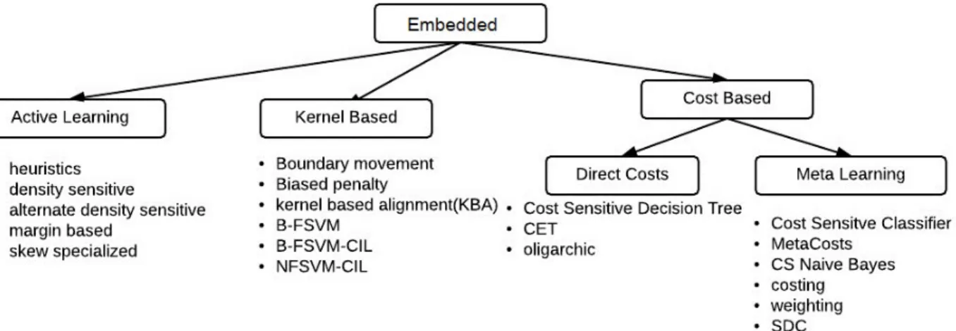
Embedded Approaches
Embedded approaches represent techniques that are usually implemented within the learner itself or during the learning phase and may be considered an internal approach. This would include techniques that apply and adjust weights or include a loss function to different samples as well as learners that inherently apply some sub-sampling selection technique. Active learning, kernel
based methods and cost assignment approaches fall into this category.
Active Learning
Active learning is a special type of semi supervised learning that allows user querying for label decisions. As part of this approach active learning will take sub-samples of existing data. It typ-ically retains samples closest to the decision boundary thus sub-sampling evenly between groups [4]. Active learning will greatly reduce the effects of imbalance but that does not mean that it will remove all the bias or guarantee improved accuracy in the under represented group.
In active learning the model is involved in selecting samples from a large pool of observations for labeling purposes and both theoretical and empirical results have shown that active learning results in highly accurate models as a result. However, these models still need to be properly tuned in order to handle class imbalanced data otherwise they will tend to inherit bias for the majority group simply because there are many more samples to choose from.
Among the most popular approaches for handling class imbalance include density sensitive ap-proaches comprised mostly of heuristic based techniques. Heuristic based apap-proaches use the entire pool of example data and assign a utility scoreU(x)denoting the improvement gained from training on that instance based on some geometric properties of the data. Popular heuristics include information density on similarity as defined in 2.56:
Um(x) =U(x)( 1 |X| n X i sim(x, xi|x6=xi))β (2.56)
Whereβis the hyper-parameter controlling the trade off between the utility scoreU(x)and the sim-ilarity scoresim(x, xi). Other heuristic based approaches include conditional probability of group
membershipUm(x) = (1− |p(y|x)|)p(x)or similarly weighted using variations of probabilistic
and similarity schemes. A number of improvements to active learning for handling imbalanced data have been researched that typically involve a similarity scoring metric based on covariates distance, cost assignments and even the use of entropy to help combat class imbalance within active learning communities [4].
Kernel Based methods
Support vector machines represent one of the core machine learning techniques that have been widely researched. These robust classifiers seem to be less sensitive to class imbalance compared to other learners when the classes are separable. As a result there has been a large amount of research utilizing SVM modifications to deal with the class imbalance problem. As previously mentioned, they have the interesting property of using kernel functions in order to perform a mapping of input attributes into a dot product space that allows for the use of many kernel types.
Wu and Chang proposed a class boundary alignment algorithm that adjusted the kernel based on the spatial distribution of the support vectors and class skew [96, 97] which was soon followed by other adjustment types including kernel target alignment, margin calibration and additional kernel modification methods which typically employ some type of loss function into the algorithm as a way of dealing with the class imbalance [10, 66, 96, 97, 57, 30, 3].
Kernel methods are not limited exclusively to SVM algorithms. Kernels are also used in Neural networks and other deep learning schemes. The kernels themselves usually implement cost based approaches which attempt to account for the importance of certain instances within the learner themselves.
Cost Assignment Approaches
This approach uses a cost or loss function for the model in order to correct class imbalance. Both the over and under represented groups have different costs applied. The goal is to shift the weight of the classifier to the under represented group thereby removing bias. The optimal prediction is thus defined by
X
j
P{j|x}C(i, j, x) (2.57)
WhereP{j|x}is the probability of observationxbelonging to classjandC(i, j, x)represents the cost for predicting classi for each examplex when the true class is j. The most difficult part is knowing the cost assignment as it may be different for every example even though the calculation formation is straight forward. A cost matrix indicating the overall benefit is usually denoted in table 2
Table 2.1: Cost Matrix
Prediction
Positive Negative
Actual
Positive C(1,1) C(0,1)
Negative C(1,0) C(0,0)
The most common approach is to assign the loss function in the problem formulation and then use the new formula on the training set. These approaches have been successfully applied to neural networks, SVMs, Naive Bayes and decision trees. Studies have empirically shown to increase the prediction accuracy of the under represented examples compared to just using the original learner
alone [55, 59, 60, 27, 100, 6].
Cost approaches can be divided into two parts direct costs and cost sensitive meta learning. Di-rect cost approaches alter the learner while meta learning approaches manipulate the training set instead. Meta learning methods can be further subdivided into sampling, threshold and MetaCosts approaches [59]. MetaCost methods attempt to change the label of the misclassified example to its optimal class as would be using equation 2.57. Sampling techniques are discussed further on and threshold approaches modify the decision threshold to account for the imbalance.
As examples of direct cost approaches, Lakshmanan et al. and Ma et al. proposed Fuzzy support vector machine approaches which apply different fuzzy membership values to account for noise and outliers as well as class imbalance into the original problem formulation [66, 57]
Akbani et al. proposed a combination of cost sensitive techniques for constructing an SVM learner with a combination of re-sampling and applied error cost for comparison [3]. Kretzschmar et al. proposed costs for each node in a neural network using marginal probabilities of a given label to control both class balance and variance [55]. Liu et al. proposed a combination of cost sensitivity and imbalance re-scale ratios [60]. All of these approaches fall under meta learning.
Boosting is another approach that falls within this category although it is an ensemble method. Boosting is an iterative algorithm that assigns weights to each training sample. For each iteration weights for incorrectly classified examples are raised while the weights with the correctly classified example are lowered. Boosting is typically a part of ensemble learning which is discussed further on.
One benefit to a cost sensitive approach is the ability to create local and global costs that can be applied in fuzzy systems with different hierarchical fuzzy regions that assign costs to particular partitions were misclassification is higher. One potential conflict is that this approach is algorithm