Evolutionary extreme learning machine for the interval type-2 radial basis function neural network: A fuzzy modelling approach

This is a repository copy of

Evolutionary extreme learning machine for the interval type-2

radial basis function neural network: A fuzzy modelling approach

.

White Rose Research Online URL for this paper:

http://eprints.whiterose.ac.uk/129567/

Version: Accepted Version

Proceedings Paper:

Rubio-Solis, A., Martinez-Hernandez, U. and Panoutsos, G. (2018) Evolutionary extreme

learning machine for the interval type-2 radial basis function neural network: A fuzzy

modelling approach. In: 2018 IEEE International Conference on Fuzzy Systems

(FUZZ-IEEE). 2018 IEEE International Conference on Fuzzy Systems (FUZZ-IEEE), 08-13

Jul 2018, Rio de Janeiro, Brazil. IEEE . ISBN 978-1-5090-6020-7

https://doi.org/10.1109/FUZZ-IEEE.2018.8491583

© 2018 IEEE. Personal use of this material is permitted. Permission from IEEE must be

obtained for all other users, including reprinting/ republishing this material for advertising or

promotional purposes, creating new collective works for resale or redistribution to servers

or lists, or reuse of any copyrighted components of this work in other works. Reproduced

in accordance with the publisher's self-archiving policy.

[email protected] https://eprints.whiterose.ac.uk/ Reuse

Items deposited in White Rose Research Online are protected by copyright, with all rights reserved unless indicated otherwise. They may be downloaded and/or printed for private study, or other acts as permitted by national copyright laws. The publisher or other rights holders may allow further reproduction and re-use of the full text version. This is indicated by the licence information on the White Rose Research Online record for the item.

Takedown

If you consider content in White Rose Research Online to be in breach of UK law, please notify us by

Evolutionary Extreme Learning Machine for the Interval Type-2 Radial

Basis Function Neural Network: A Fuzzy Modelling Approach

Adrian Rubio-Solis

, Uriel Martinez-Hernandez

and George Panoutsos

Abstract— It has been demonstrated that Evolutionary Ex-treme Learning Machine (E-ELM) is frequently much more efficient than traditional gradient-based algorithms for the parameter identification of feedforward neural networks. In particular, E-ELM is usually faster and provides a higher trade-off between accuracy and model simplicity. For that reason, this paper shows that an E-ELM that is based on Particle Swarm Optimisation (PSO) and Extreme Learning machine (ELM) can be extended to the Interval Type-2 Radial Basis Function Neural Network (IT2-RBFNN) with a Karnik-Mendel type-reduction layer. To evaluate the efficiency of E-ELM, the IT2-RBFNN is used as an Interval Type-2 Fuzzy Logic System (IT2 FLS) for the modelling of two popular data sets and for the prediction of chaotic time series. According to our results, E-ELM applied to the IT2-RBFNN not only outperforms adaptive-gradient-based algorithms and provide a better generalisation compared to other existing IT2 fuzzy methodologies, but similarly to pure fuzzy models, the IT2-RBFNN is also able to preserve some model interpretation and transparency.

Index Terms— Interval type-2 fuzzy logic systems. RBF neural networks, extreme learning machine, Particle Swarm Optimisation (PSO), fuzzy modelling.

I. INTRODUCTION

Fuzzy Logic Systems (FLSs) have been widely used to solve a large number of real world problems [1–5]. In partic-ular, in the areas of function approximation and classification problems, FLSs of Interval Type-2 (IT2) have demonstrated to be more efficient to handle with uncertainties, such as nosiy and sparse data as well as their ability to operate under disturbances that usually T1 FLSs can not [5, 6]. Moreover, Adaptive Fuzzy Inference Systems (AFISs) based on the fusion of IT2 FLSs and Neural Networks (NNs) not only inherit the ability to deal with uncertainty, but also adaptive-ness, generalisation properties, fault tolerance, approximate reasoning under cognitive uncertainty [7]. The Interval Type-2 Radial Basis Function Neural Network (ITType-2-RBFNN) is a neural structure that can be viewed as a Interval Type-2 Fuzzy Logic System and that inherits the ability of NNs for function approximation of piecewise continuous real-valued mappings, and the ability of FLSs to use an inference engine as the fuzzy rule generation criterion [5]. Until now, the parameter identification for the IT2-RBFNN has been based on gradient-based optimisation algorithms that require a high number of mathematical formulas to compute the

1

A. Rubio-Solis is with the department of Automatic Control and Systems (ACSE), The University of Sheffield, Sheffield, S1 3JD United [email protected]

2

Uriel Martinez-Hernandez is with the Institute of Design, Robotics and Optimisation (iDRO), School of Mechanical Engi-neering, University of Leeds, Leeds, LS2 9JT, United Kingdom.

[email protected]

associated derivatives. This computation results much more complicated for an IT2-RBFNN with a Karnik-Mendel (KM) type reducer. Especially, because a KM algorithm requires a reordering process that creates a number of permutations which must be tracked during the learning process [8]. Due to its simplicity and applicability to train a wider type of Single Layer Feedforward Networks (SLFNs), Extreme Learning Machine (ELM) has gained a lot of popularity during the last decade [9, 10]. ELM provides a higher generalisation performance and compared to gradient-descent learning al-gorithms, it avoids getting trapped in local minima while decreasing the associated computational load. Particularly for the Radial Basis Function Neural Network (we call it RBFNN of type-1), it has been proven a higher efficiency and better performance compared to the gradient descent approach. However, compared to traditional approaches, the implementation of ELM still requires a higher number of hidden units to train a SLFN as a consequence of the random estimation of the input weights and hidden unit parameters [11, 12]. To overcome those drawbacks of ELM, a number of hybrid approaches based on evolutionary optimisation algorithms and ELM have been proposed [13–17].

In this paper the main target is to extent E-ELM to the Interval Type-2 Radial Basis Function Neural Network (IT2-RBFNN) case. To find the optimal parameters of the antecedent and consequent parts of the IT2-RBFNN, we use a Particle Swarm Optimisation (PSO) and Extreme Learning Machine theory (ELM) respectively. To test the efficiency of the IT2-RBFNN and E-ELM, we use two complex and popular data sets from the UCI repository and the Mackey-Glass chaotic time series. The resulting IT2-RBFNN is com-pared to other existing IT2 neural structures such as an IT2-RBFNN with a KM type reduction and including Support Vector Machines (SVM) and the RBFNN. According to our results, the utilisation of an Evolutionary Extreme Learning approach (E-ELM) enhances the generalisation properties of the IT2-RBFNN while preserving the model interpretation and ransparency that pure fuzzy models usually offer.

The rest of this paper is organised as follows: in section II, a brief review of Extreme Learning Machine (ELM) for Single Layer Feedforward Networks (SLFNs) and Particle Swarm Optimisation (PSO) is provided. Section III, de-scribes the functional equivalence between IT2 FLSs and the IT2-RBFNN. Experimental results are compared in section IV, and finally section V draws the conclusions.

II. RELATEDWORK

This section provides a brief review of Extreme Learning Machine theory for Single Layer Feed-forward Networks (SLFN) and the Particle Swarm Optimisation algorithm (PSO).

A. Extreme Learning Machine for SLFNs

According to the basics of ELM [9, 10], for a number of

P different samples (xp, yi)Pp=1 ⊂Rn×RP, Single Layer Feed-forward Networks (SLFNs) can be mathematically ex-pressed as: ˜ N X i=1 βigi(xp) = ˜ N X i=1 βig(wi·xp+bi) =yp (1)

in which xp = [xp1, . . . , xpn] is the input vector, wi =

[wi1, . . . , win]T and βi = [βi1, . . . , βip] are the weight vectors that connects theithhidden node to the input and to the output nodes respectively. A SLFN withN˜ hidden nodes and activation functiong(x)can approximatePsamples with zero error meansPM_p=1kyp−tpk. Thus, the set of equations described in (10) can be written compactly as:

H(w1, . . . , wN˜, b1. . . , bN˜, x1, . . . , xP) =    g(w1·x1+b1) · · · g(w1·x1+b1) .. . ... ... g(w1·xP+b1) · · · g(wN˜·xP +bN˜)    P×N˜ β=    β1T .. . β_NT˜    ˜ N×n and Y =    yT 1 .. . yT P    P×n (2)

WhereHis the hidden layer output matrix of a SLFN with respect to the input xp. Thus, the minimum norm least-squares solution of the linear system Hβ = T is unique and can be achieved by calculating the pseudoinverse H†

as:

ˆ

β=H†T (3)

B. Particle Swarm Optimisation

Particle Swarm Optimisation (PSO) has demonstrated to be an efficient population-based stochastic optimisation technique originally developed by Eberhart and Kennedy [18, 19]. PSO mimics the societal behaviour of some species such as fish, birds and some mammals to flocking while obtaining individual benefits. PSO initialises with a flock of birds usually called particles that are randomly selected. Every jth particle flies with an specific velocity vj while keeping track of its best position pbest. Thus, at each time step, each particle changes its velocity and position (direction)xˆjtowards the best locationxˆbest. The associated acceleration of each particle is weighted by a random term. Hence, the velocity and position is defined

vj=wdvj+c1rp(pbest,j−xˆj) +c2rg(gbest−xˆj) (4)

ˆ

xj = ˆxj+vj;j= 1, . . . , np (5)

where c1 and c2 are acceleration constants with positive values; rp and rg are random numbers between 0 and 1. The termwd is used for adaptation purposes as an inertial weight. Such parameter is decreased gradually as the number of generation for the PSO increases according to the rate:

wd(t) =(

wmax−winit)

M axT

(6) in which, winit and wmax are the initial and final inertial weights respectively.

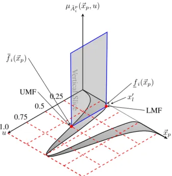
III. RADIALBASISFUNCTIONNEURALNETWORK AND INTERVALTYPE-2 FUZZYLOGICSYSTEMS As described in [20], a Radial Basis Function Neural Network (RBFNN) can be viewed as a Type-1 Fuzzy Logic System of either Mamdani or Takagi-Sugeno-Kang type (TSK) under some mild restrictions. This equivalence has been extended in [5] in order to design an RBFNN that is functionally equivalent to an Interval Type-2 FLS with a Karnik-Mendel type-reduction in which all the fuzzy sets are interval type-2 fuzzy sets (IT2 FSs). An RBFNN can be regarded as an FLS whose main inference engine is interpreted as an adaptive filter [21, 22]. According to [21], the fired-rule output sets in the hidden layer of an RBFNN resemble an additive weighted combination of the MFs [21]. Thus, as illustrated in Fig. 1, each hidden receptive unit in the RBFNN is functionally equivalence to a fuzzy rule Ri described by a multi-variable MF µRi(x_p, y_p) =

µRi[x₁, . . . , x_n, y]of Gaussian type, where the input vector

xp= [x1, . . . , xn]∈X1×. . . Xn and the implication engine can be defined as:

µRi(x_p, y) =µ_Ai_→Gi = T_s=1N µFi s(xs)⋆ µGi(y) (7) Where⋆is the minimumt−normthat represents the shortest Euclidean distance of the input vectorxp in which the ith receptive unit is represented as a fuzzy rule in the form:

Ri:IFx1 isF1i and. . .IFxsis Fsi and. . .

IFxN is FNi THENy isGi; i= 1, . . . , M (8) Therefore, the firing strength fi of each receptive unit is defined as: µAi_→Gi(x_p, y) = n Y s=1 µFi s(xs) (9) =f i exp " − Pn s=1(xs−msi) 2 σ2 i #! (10) Strictly speaking, any kind of FLS enhancement might be directly applicable to the RBFNN theory because the structure of its fuzzy rule base (receptive units) in going from T1 FSs to IT2 FSs does not change; it is the way the associated antecedents and consequents are modelled [8]. Therefore, an RBFNN can be functionally equivalence to an IT2 FLS if an RBFNN consists of:

I. An input layer with a singleton fuzzification.

II. The T-norm operator used to compute each rule’s firing strength is multiplication (meet).

~ xp u µ_A˜p i(~xp, u) V ertical Slice 1.0 0.75 0.5 0.25 fi(~xp) LMF fi(~xp) UMF x′ l • •

Fig. 1:Singleton fuzzification and triangle secondary MF that is activated whenx_p=x′

lfor theithreceptive unit of the IT2-RBFNN

III. The output of each MF is an IT2 FS that is defined by a lower and upper MF.

IV. The output weight is an interval[wi

l, wir](or a constant

wi).

A. Interval Type-2 Radial Basis Function Neural Network

Based on the functional equivalence between the RBFNN and IT2 FLSs [5, 23], in this paper, an Interval Type-2 Radial Basis Function Neural Network (IT2-RBFNN) having a center-of-sets type reduction, product inference rule and a singleton output space is used. The type-reduced set

(yl, yr) is obtained by using a Karnik-Mendel algorithm [24]. According to Fig. 2, if wi is a crisp value and the IT2-RBFNN is either of Mamdani or TSK type, the matrix representation of the IT2-RBFNN output can be written as [8, 25]:

yf =

1

2(Yl+Yr)w

T ₍₁₁₎

in which yl=YlwT andyr=YrwT and

Yl= fTQT_ET 1E1Q+fTQTE2TE2Q rT lQf+sTl Qf (12) whereYl= (ψl,1, . . . , ψl,M) E1= (e1|e2|. . .|eL|0|. . .|0)T L×M E2= (0|. . .|0|ξ1|ξ2|. . .|ξM−L)T (M−L)×1 rl≡(1,1, . . . ,1 | {z } L ,0, . . . , . . . ,0)T _M×1 sl≡(0, . . . , . . . ,0 M−L z }| { 1,1, . . . ,1)T M×1 X 1 X 2 X 3 X s X n f 3 f 3 f 1 f 1 f 2 f 2 f i f M f i f M y l y_r y_p w i Interval RBF layer Type-reduction layer

Input vector layer

Fig. 2: Interval Type-2 Mamdani Radial Basis Function with an Karnik Mendel type-reduction.

with ej ∈ RL (j = 1, . . . , L) and ξj ∈ RM−L, j =

1, . . . , M − L as the elementary vectors where all the elements are zero except thejthone that is equal to 1.

Yr= fTQTE3TE3Q+fTQTE4TE4Q rT rQf+sTl Qf (13) whereYr= (ψr,1, . . . , ψr,M) E3= (e1|e2|. . .|eR|0|. . .|0)T R×M E4= (0|. . .|0|ξ1|ξ2|. . .|ξM−R)T (M −R)×1 rr≡(1,1, . . . ,1 | {z } R ,0, . . . , . . . ,0)T _{M ×1} sr≡(0, . . . , . . . ,0 M−R z }| { 1,1, . . . ,1)T M ×1 with ej ∈ RR (j = 1, . . . , R) and ξj ∈ RM−R, j =

1, . . . , M − R as the elementary vectors where all the elements are zero except the jth one that is equal to 1.

f= (f1, . . . , fM)T,f= f1, . . . , fM, T

. By using Karnik-Mendel algorithms [24], the reordered consequent weights

˜w that results from the permutation process to find the switching points L and R can be calculated according to [25]

˜

w=QwT, Q∈RM×M (14) In which w = (w1, . . . , wM) is the set of original rule-ordered consequent weights and Q is the corresponding permutation matrix [25]. The ith fuzzy rule of an IT2-RBFNN is written as

˜

Ri:IFx1 isF1i and. . .IFxsis Fsi and. . .

IFxn isFni THENy iswi; i= 1, . . . , M (15) For an IT2-RBFNN of Mamdani type wi is a single crisp value, while for a TSK modelwi=ci0+ci1x1+ci2x2+. . .+

cinxn. For each rule in the IT2-RBFNN, its interval firing strengthFi _{for a Gaussian function having a fixed meanm}i s

and anuncertain standard deviation[σ1

i, σ2i]whenxs=x′l and computed as:

Fi:=                Fi_{= [f} i(~xp), fαis(~xp)] fi(~xp) =exp " − n X k=1 xs−mis σ2 i 2# fi(~xp) =exp " − n X s=1 xs−mis σ_i1 2# (16)

IV. EVOLUTIONARYEXTREMELEARNING FOR AN INTERVALTYPE-2 RBFNN

In Neural Networks applications, the implementation of ELM usually requires a higher number of hidden neurons due to the random estimation of input weights and hidden biases that may cause the computation of unnecessary parameters. Thus, in order to determine a reduced number of optimal parameters for the IT2-RBFNN with a Gaussian MF having a fixed meanmsiand a variable standard deviation[σ1i, σ22], in this section we apply an Evolutionary Extreme Learning Machine methodology (E-ELM for short) that is based on the Particle Swarm Optimisation (PSO) and ELM theory. According to algorithm 1, given a predefined number of fuzzy rules, the PSO starts from randomly selecting the values of each IT2 antecedent whose particle’s codification

ˆ

xj∼U(lj, uj)is shown below (line 2), wherelj anduj are the lower and upper dimension limits respectively.

ˆ xj =    IT2 antecedent 1 z }| { m11, . . . , mn1, σ11, σ21, . . . , IT2 antecedent n z }| { m1M, . . . , mnM, σ11, σ21 | {z } Rule 1 , . . . , IT2 antecedent 1 z }| { m11, . . . , mn1, σM1 , σ2M, . . . , IT2 antecedent n z }| { m1M, . . . , mnM, σ1M, σM2 | {z } Rule M   

in which Np is the number of particles. ForP input-output data vectors (~xp, dp), p = 1, . . . , P, the fitness of each candidate model Jt(ˆxj)is the Root-Mean-Squared-Error of each candidate model (line 3)

Jt(xj) = 1 P P X p=1 (yp−tp)2 !1/2 (17) At each iteration of the PSO (line 9-12), the updated position of each particle is used as the set of the antecedent parts of each new IT2-RBFNN model. Therefore, ELM is system-atically called in two different steps in order to update the consequent weights of each candidate model [17]. At first step [6], the optimal inital values for the consequents are obtained by approximating the reduced set[yl, yr]as:

yl,1= PM i=1fiwi PM i=1fi = M X i=1 f′_iwi; f′i = fi PM i=1fi (18) yr,1= PM i=1fiwi PM i=1fi = M X i=1 f′ iwi; f′i= fi PM i=1fi (19) By using Eq. (12) and (13), the following linear system can

Algorithm 1:PSEUDOCODE FOR THE EVOLUTIONARY EX-TREME LEARNING METHODOLOGY FOR THE IT2-RBFNN

Input: Input Training Data(xp, tp)

Output:Optimal IT2 antecedentsmsi, σi and consequent weights gi

1 functionParticle Swarm Optimisation (PSO)

2 Initialise a setS_p of N_p random particle’s position:

ˆ

xj∼U(lj, uj)

3 CalculateJt(ˆxj), j= 1, . . . , Np

4 Initialise the particle’s best positionpbest,j←xˆj 5 whilet≤ M axT do

6 forallxˆj∈Sp do

7 Update particle’s velocityvj←wdvj+

c1rp(pbest,j−xˆj) +c2rg(gbest−xˆj) 8 Update particle’s positionxˆ_j ←xˆ_j+v_j 9 Calculatew= Φ(x)†Yat iterationj 10 Calculate fitnessJ_t(ˆx_j)

11 Select the best antecedent and consequent parameters

12 ifJ_t(x_p)< p_best,j then

13 Update the particle’s best position

xbest,j←xˆj

14 ifp_best,j< g_best then

15 Update the best known position

xbest←xbest,j

16 t=t+ 1

17 return(m_si, σ1_i, σ_i2,ˆc)_best

be written for a number ofP patterns:

Y= Φ1(x)w (20)

in which, x = {xp|p = 1, . . . , P}, xp = [xp1, . . . , xpn] andYis the desired output vector, wherenis the number of input variables. For a IT2-RBFNN with a TSK (Mamdani) fuzzy rule structure, the matrixΦcan be written as.

Φ1(x) =      Φ1 Φ2 .. . Φp      ∈RP×M(n) (21)

From Eq. (18) and (19) it follows for a TSK implication:

Φpw= 1 2 M X i=1 (f′i+f′i) n X s=1 cisxs ! (22) For an IT2-RBFNN of Mamdani type, the second addition term in Eq. (22) is a single crisp value wi. Therefore, the solution to the linear system described in Eq. (20) is calculated as follows:

w1= Φ1(x)†Y (23) wherew1 is the optimal initial value for the consequent vec-torw andΦ1(x)† is the Moore-Penrose generalised inverse of Φ1(x). Secondly, the final optimisation of w consists of

implementing the KM algorithm. From Eq. (12) and (13) the terms Yl and Yr are used to calculate w that can be expressed as the linear system:

Y= Φ2(x)w (24) Such as Φ2(x) =      Φ1 Φ2 .. . Φp      ∈RP×M(n) (25) in which Φpw= 1 2 M X i=1 (ψl,i+ψr,i) n X s=1 cisxs ! (26) Andwis obtained by finding the correspondingΦ†2 as

w= Φ2(x)†Y (27) After one iteration of the PSO, each IT2 antecedent in the IT2-RBFNN is updated by using the particle’s position xˆj that produce the best fitnessJt(ˆxj)(line 7-10). Finally, the codification of the best candidate model (particle’s position) is used as the optimal set of values formsi,[σi1, σ2i]andcsi or wi if the IT2-RBFNN is of Mamdani type (line 18).

V. EXPERIMENTALRESULTS

In this section, the performance of the proposed E-ELM for the optimisation of the antecedent and consequent parts of the IT2-RBFNN having afixed meanmsi and avariable

standard deviation [σi1, σ2i] is compared to other techniques such as an IT2-RBFNN trained with an Adaptive Gradient Descent (AGD) approach [5, 23, 26], Support Vector Ma-chines (SVMs), Back propagation networks (BPNs), RBFNN and an Interval Type-2 Fuzzy Neural Network with Support Vector Regression. We use two complex data sets from the UCI repository, i.e. 1) the High-performance Concrete (HPC) data set for the prediction of compressive strength [27, 28] and 2) the Parkinson telemonitoring data set for the diagnosis of patients having or not Parkinson’s disease. Finally, we evaluate the E-ELM and the IT2-RBFNN for noisy regression prediction using the Mackey-Glass chaotic time series [6].

A. Example 1: High-Performance Concrete (HPC) Compres-sive Strentgh Prediction

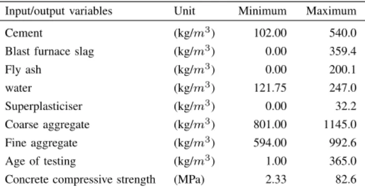
In this example, the performance of the E-ELM and the IT2-RBFNN for the prediction of HPC compressive strength is studied. The main difference between HPC and conventional concrete lies on the use of mineral and chemical admixture. Due to its nonlinearity with respect to age, ingredients and those admixtures, the HPC is a difficult and highly complex behaviour to be predicted. HPC is a composite in construction industry whose basic composition includes cement, fine coarse aggregate and water. The HPC data set is a regression problem that consists of 1030 samples with 8 inputs each whose general details are presented in Table I.

TABLE I:General details of the HPC compressive strength data set. Input/output variables Unit Minimum Maximum

Cement (kg/m3

) 102.00 540.0

Blast furnace slag (kg/m3

) 0.00 359.4 Fly ash (kg/m3 ) 0.00 200.1 water (kg/m3 ) 121.75 247.0 Superplasticiser (kg/m3 ) 0.00 32.2 Coarse aggregate (kg/m3 ) 801.00 1145.0 Fine aggregate (kg/m3 ) 594.00 992.6 Age of testing (kg/m3_{) 1.00 365.0}

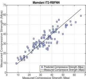
Concrete compressive strength (MPa) 2.33 82.6 For cross-validation reasons, the HPC data set is divided into two subsets, i.e. 90%for training and 10%for testing. Unlike the results presented in [27, 28], we perform a number of 20 random experiments and the average RMSE is used to evaluate the IT2-RBFNN efficiency. As shown in Table II, the model accuracy of the IT2-RBFNN models based on E-ELM and an AGD approach [29] are compared to a Support Vector Machine (SVM) [27, 28], a Back-Propagation Network (BPN) [27, 28] and an Evolutionary Fuzzy Support Vector Machine Inference Model (ESFIM) [27, 28] that uses a number of linear, quadratic or exponential time series functions for the parameter identification of the SVMs. The experimental setup consists of a number of 300 evolution generations for the E-ELM, a number of 8 IT2 fuzzy rules for the IT2-RBFNN and the input data was normalised to the interval[0−1]. From our simulation results in Table II, it is clear that the best generalisation performance is achieved by using a Mamdani IT2-RBFNN based on E-ELM. To exem-plify the ability of the most accurate IT2-RBFNN to provide some physical interpretation about the HPC data set, the data-fit for the testing stage and the effect surface response that corresponds to the ingredients cement and superplasticiser are presented in Fig. 3 and 4, respectively. This is achieved by keeping(n−1)input variables constant and plotting the remaining variables agaisnt the HPC compressive strength. Usually the variables that are kept constant use their average or the dominat value of their corresponding input dimension. This is mainly due to the nature of the data and its associated sparsity.

TABLE II:Comparison performance between the IT2-RBFNN, EFSIM, SVM and BPN.

Model Type-reduction Training Testing

EFSIM Linear 5.120 5.865 Quadratic 5.126 5.378 Exponential 5.152 5.430 SVM [27] 8.854 10.406 BPN [27] 5.094 6.900 IT2-RBFNN

Adaptive Gradient Descent Methodology (AGD)

Mamdani KM 5.010 5.170

TSK KM 5.871 5.392

Evolutionary Extreme Learning Machine (E-ELM)

Mamdani KM 5.636 4.735

Measured Compressive Strength (Mpa)

0 10 20 30 40 50 60 70

Measured Compressive Strength (Mpa)

0 10 20 30 40 50 60 70 Mamdani IT2-RBFNN

Predicted Compressive Strength (Mpa) Measured Compressive Strength (Mpa)

Fig. 3: Data-fit for a random testing experiment for the HPC concrete compressive strength using an IT2-RBFNN based on E-ELM.

600 500 Cement (kg/m3) 400 300 200 100 100 Superplasticiser (kg/m3) 150 200 80 70 60 50 40 30 20 250 Concrete Compressive Strength (MPa)

Fig. 4:Surface response for the Superplasticiser and Cement ingredients.

B. Example 2: Parkinson Telemonitoring Data Set

This data set consists of a collection of biomedical voice measurements from a number of 31 patients, 23 with Parkin-son’s disease (PD). The purpose of this example is to evaluate the classification accuracy of the IT2-RBFNN based on E-ELM to diagnose a patient with PD or not. We compare its performance to an IT2-RBFNN that is trained with AGD, three different types of Probabilistic Neural Networks (PNN) whose main optimisation process is based on an incremental search (IS), Monte Carlo method (MC) [30] and a hybrid search [31–33]. To quantify the model accuracy, we use the following metrics:a) specificity, b) sensitivity and c) accuracy. While specificity measures the number of patients without PD (TA), sensitivity measures the proportion of patients with PD (TP) that are correctly classified. Accuracy is the overall percentage that both categories of diagnosis are correctly classified.

Specif icity= T A

T A+F P (28) Sensitivity= T P

F A+T P (29)

TABLE III:Comparison performance between the IT2-RBFNN, EFSIM, SVM and BPN.

Model Type-reduction Training

accuracy Testing accuracy PNN-IS [31] 81.73% 79.78% PNN-MC [31] 81.48% 80.92% PNN-HS [31] 81.74% 81.28% IT2-RBFNN

Adaptive Gradient Descent Methodology (AGD)

Mamdani KM 89.74% 88.33%

TSK KM 89.91% 87.58%

Evolutionary Extreme Learning Machine (E-ELM)

Mamdani KM 97.10% 93.07%

TSK KM 98.07% 92.29%

WhereFPandFArepresent false prediction for the pres-ence and abscpres-ence of PD respectively. For cross validation purposes, the PD data set was divided into two subsets,70%

for training and 30% for testing. A number of 20 random simulations was performed, and the mode average accuracy is presented in Table III. From these reults, the application of an E-ELM confirms its superiority as an heuristic search to enhance the performance and adaptation of the IT2-RBFNN.

C. Example 3: Noisy Chaotic Time-Series Prediction

As the last experiment, we use a time-series prediction problem to evaluate the performance of the IT2-RBFNN. We employ the Mackey-Glass chaotic time series which is generated from the following differential equation [?]:

dx(t)

dt =

0.2x(t−τ)

1 + 10x(t−τ)−0.1x(t) (30)

For comparison reasons with previous results, we use the parameters τ = 30, x(0) = 1.2. Four past values were employed to predictx(t)where the input data format is used as:

[x(t−24), x(t−18), x(t−12), x(t−6);x(t)]

A number of 1000 patterns were generated from the obser-vation t= 124 to t = 1123. For cross-validation purposes, the input data was divided into two subsets, i.e. a)50% for training and b)50% for testing and a number of20random experiemnts were carried out. To compare the performance of the IT2-RBFNN and the E-ELM to other existing IT2 methodologies, two different types of training data were created by adding a Gaussian noise with a standard deviation ofσ= 0.2andσ= 0.3with a mean of0to the original data

x(t). This type of noise has been selected because it usually occurs in real situations and it is frequently employed to verify model robustness [6]. For testing data, three data sets were created from the original data set. The first consists of the original 500 values. The last two testing data sets were created by adding a Gaussian noise with a σ = 0.2

andσ = 0.3 . From Table IV and V, row clean is used to show those results that correspond to the data with no noise. We divided the simulation results according to the type of implication engine, i.e. of a Mamdani or b) TSK type.

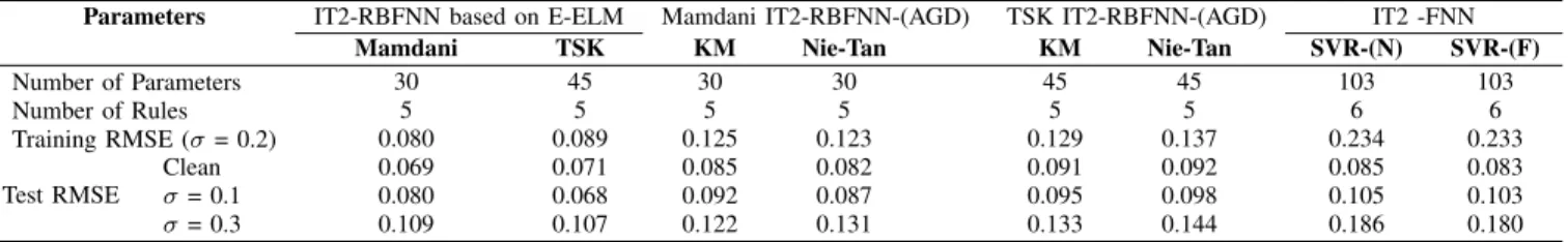
TABLE IV:Performance of the IT2-RBFNN based on E-ELM and other models with a training noiseσ_{= 0.2 in example 3.}

Parameters IT2-RBFNN based on E-ELM Mamdani IT2-RBFNN-(AGD) TSK IT2-RBFNN-(AGD) IT2 -FNN

Mamdani TSK KM Nie-Tan KM Nie-Tan SVR-(N) SVR-(F)

Number of Parameters 30 45 30 30 45 45 103 103 Number of Rules 5 5 5 5 5 5 6 6 Training RMSE (σ_{= 0.2) 0.080 0.089 0.125 0.123 0.129 0.137 0.234 0.233} Test RMSE Clean 0.069 0.071 0.085 0.082 0.091 0.092 0.085 0.083 σ_{= 0.1 0.080 0.068 0.092 0.087 0.095 0.098 0.105 0.103} σ_{= 0.3 0.109 0.107 0.122 0.131 0.133 0.144 0.186 0.180}

TABLE V:Performance of the IT2-RBFNN based on E-ELM and other models with a training noiseσ_{= 0.3 in example 3.}

Parameters IT2-RBFNN based on E-ELM Mamdani IT2-RBFNN-(AGD) TSK IT2-RBFNN-(AGD) IT2 -FNN

Mamdani TSK KM Nie-Tan KM Nie-Tan SVR-(N) SVR-(F)

Number of Parameters 30 45 30 30 45 45 103 103 Number of Rules 5 5 5 5 5 5 6 6 Training RMSE (σ_{= 0.3)} 0.080 0.089 0.133 0.138 0.152 0.145 0.349 0.347 Test RMSE Clean 0.070 0.078 0.092 0.094 0.101 0.105 0.127 0.121 σ_{= 0.1 0.101 0.094 0.127 0.139 0.133 0.143 0.138 0.131} σ_{= 0.3 0.119 0.121 0.144 0.155 0.147 0.161 0.188 0.184} Time Step 0 100 200 300 400 500 Output Prediction 0.4 0.5 0.6 0.7 0.8 0.9 1 1.1 1.2 1.3

1.4 TSK IT2-RBFNN based on E-ELM

Measured Output Predicted Output

Fig. 5:Data fit of a dandom experiment for the prediction of the Mackey-Glass chaotic time series using a TSK IT2-RBFNN based on E-ELM.

To compare the IT2-RBFNN performance, we use the results obtained by three different interval type-2 fuzzy mod-elling methodologies, namely: a) an IT2FNN-SVR-(N), b) an IT2-FNN-SVR-(F) and an c) KM IT2-RBFNN. The first two models a) and b) were introduced in [6]. The IT2-FNN-SVR is a six-layer interval type-2 fuzzy neural network with support vector machine regression that uses two different types of input nodes. For the first type, the input nodes in an IT2-FNN-SVR simply forwards each numerical data and is called IT2-FNN-SVR-(N) for short. Thus, the output of the IT2-FNN-SVR-(N) is a bounded interval which is described in terms the lower and upper limits of its Footprint Of Uncertainty (FOU). An IT2-FNN-SVR-(F) uses an input node layer that fuzzifies the input numerical data. The third IT2 methodology is an IT2-RBFNN with a Karnik-Mendel (KM) type-reduction layer and an IT2-RBFNN with a direct defuzzification method based on the Nie-Tan approach whose parameter optimisation is based on an AGD and that we call in this example IT2-RBFNN-(AGD) for short. According

to our results, it is evident from Table IV and V, the IT2-RBFNN based on E-ELM outperforms the rest of the neural models. In Fig. 5, the testing data-fit for a TSK IT2-RBFNN based on E-ELM is shown. Finally, in Fig. 6 and 7, the initial and final distribution for the first 4 IT2 fuzzy sets for the inputx(t−24)is illustrated.

input:x(t−24) µAp i(xp, u) u F 1 1 F12 F3 1 F4 1 0.5 1.0 1.0

Fig. 6:Initial Membership Functions for the inputx₍t_−24).

input:x(t−24) −µA˜p i(xp, u) µA˜p i(xp, u) u 0.5 1.0 1.0 ˜ F1 1 F˜₁4 _F˜3 1 _F˜2 1

VI. CONCLUSIONS

In this paper, an Evolutionary Extreme Learning Machine (E-ELM) that is based on Particle Swarm Optimisation (PSO) and Extreme Learning Machine (ELM) theory is extended to the Interval Type-2 Radial Basis Function Neural Network (IT2-RBFNN) case. To evalute the effectiveness of the E-ELM, IT2-RBFNN, was applied to model two complex data ses from the UCI repository and for the noisy prediction chaotic time series. A comparion about the performance of the IT2-RBFNN to some existing IT2 fuzzy methodologies such as fuzzy support vector regression, the IT2-RBFNN trained with an Adaptive Gradient Descent (AGD) as well as Backpropagation Neural Networks (BPN) is provided. Compared to traditional gradient descent approaches, the implementation of an E-ELM eliminates the initial condition selection for the antecedent parts that is usually required to train an IT2-RBFNN. Moreover, based on our simulation results, the IT2-RBFNN trained with an E-ELM not only enhances its generalisation accuracy, but also preserves the ability of Fuzzy Logic Systems (FLS) to provide a good trade-off between model interpretation and simplicity.

Under similar structural and parametric conditions, in the future, we are planning to study other type of T2 neural structures that simplify the implementation of E-ELM. This includes the design and implementation of new learning methodoloiges that reduce the associated computational load and its associated complexity.

REFERENCES

[1] E.-H. Kim, S.-K. Oh, and W. Pedrycz, “Design of reinforced interval type-2 fuzzy c-means-based fuzzy classifier,”IEEE Transactions on

Fuzzy Systems, 2017.

[2] M. de los Angeles Hernandez, P. Melin, G. M. M´endez, O. Castillo, and I. L´opez-Juarez, “A hybrid learning method composed by the orthogonal least-squares and the back-propagation learning algorithms for interval a2-c1 type-1 non-singleton type-2 tsk fuzzy logic systems,”

Soft Computing, vol. 19, no. 3, pp. 661–678, 2015.

[3] E. Rubio, O. Castillo, and P. Melin, “Interval type-2 fuzzy system design based on the interval type-2 fuzzy c-means algorithm,” inFuzzy

Technology. Springer, 2016, pp. 133–146.

[4] E. Rubio, O. Castillo, F. Valdez, P. Melin, C. I. Gonzalez, and G. Mar-tinez, “An extension of the fuzzy possibilistic clustering algorithm using type-2 fuzzy logic techniques,”Advances in Fuzzy Systems, vol. 2017, 2017.

[5] A. Rubio-Solis and G. Panoutsos, “Interval type-2 radial basis function neural network: a modeling framework,”IEEE Transactions on Fuzzy

Systems, vol. 23, no. 2, pp. 457–473, 2015.

[6] C.-F. Juang, R.-B. Huang, and W.-Y. Cheng, “An interval type-2 fuzzy-neural network with support-vector regression for noisy regression problems,” IEEE Transactions on fuzzy systems, vol. 18, no. 4, pp. 686–699, 2010.

[7] Q. Fan, J. M. Zurada, and W. Wu, “Convergence of online gradient method for feedforward neural networks with smoothing l 1/2 regu-larization penalty,”Neurocomputing, vol. 131, pp. 208–216, 2014. [8] J. M. Mendel, “General type-2 fuzzy logic systems made simple: a

tutorial,” IEEE Transactions on Fuzzy Systems, vol. 22, no. 5, pp. 1162–1182, 2014.

[9] G.-B. Huang, Q.-Y. Zhu, and C.-K. Siew, “Extreme learning machine: theory and applications,”Neurocomputing, vol. 70, no. 1, pp. 489–501, 2006.

[10] G.-B. Huang, H. Zhou, X. Ding, and R. Zhang, “Extreme learning machine for regression and multiclass classification,”IEEE

Transac-tions on Systems, Man, and Cybernetics, Part B (Cybernetics), vol. 42,

no. 2, pp. 513–529, 2012.

[11] L. Yingwei, N. Sundararajan, and P. Saratchandran, “A sequential learning scheme for function approximation using minimal radial basis function neural networks,”Neural computation, vol. 9, no. 2, pp. 461– 478, 1997.

[12] W.-Y. Deng, Q.-H. Zheng, L. Chen, and X.-B. Xu, “Research on extreme learning of neural networks,”Chinese Journal of Computers, vol. 33, no. 2, pp. 279–287, 2010.

[13] S. Li, P. Wang, and L. Goel, “Short-term load forecasting by wavelet transform and evolutionary extreme learning machine,”Electric Power

Systems Research, vol. 122, pp. 96–103, 2015.

[14] Y. Xu and Y. Shu, “Evolutionary extreme learning machine–based on particle swarm optimization,”Advances in Neural Networks-ISNN 2006, pp. 644–652, 2006.

[15] F. Han, H.-F. Yao, and Q.-H. Ling, “An improved evolutionary extreme learning machine based on particle swarm optimization,”

Neurocomputing, vol. 116, pp. 87–93, 2013.

[16] J. Cao and L. Xiong, “Protein sequence classification with improved extreme learning machine algorithms,”BioMed research international, vol. 2014, 2014.

[17] Z. Deng, K.-S. Choi, L. Cao, and S. Wang, “T2fela: type-2 fuzzy extreme learning algorithm for fast training of interval type-2 tsk fuzzy logic system,” IEEE transactions on neural networks and learning

systems, vol. 25, no. 4, pp. 664–676, 2014.

[18] R. Eberhart and J. Kennedy, “A new optimizer using particle swarm theory,” in Micro Machine and Human Science, 1995. MHS’95.,

Proceedings of the Sixth International Symposium on. IEEE, 1995,

pp. 39–43.

[19] J. Kennedy, “Particle swarm optimization,” inEncyclopedia of

ma-chine learning. Springer, 2011, pp. 760–766.

[20] J.-S. Jang and C.-T. Sun, “Functional equivalence between radial basis function networks and fuzzy inference systems,”IEEE transactions on

Neural Networks, vol. 4, no. 1, pp. 156–159, 1993.

[21] J. M. Mendel, “Fuzzy logic systems for engineering: a tutorial,”

Proceedings of the IEEE, vol. 83, no. 3, pp. 345–377, 1995.

[22] A. R. Solis and G. Panoutsos, “Granular computing neural-fuzzy mod-elling: A neutrosophic approach,” Applied Soft Computing, vol. 13, no. 9, pp. 4010–4021, 2013.

[23] A. Rubio-Solis, G. Panoutsos, and S. Thornton, “A data-driven fuzzy modelling framework for the classification of imbalanced data,” in

Intelligent Systems (IS), 2016 IEEE 8th International Conference on.

IEEE, 2016, pp. 302–307.

[24] D. Wu and J. M. Mendel, “Enhanced karnik–mendel algorithms,”IEEE

Transactions on Fuzzy Systems, vol. 17, no. 4, pp. 923–934, 2009.

[25] J. M. Mendel, “Computing derivatives in interval type-2 fuzzy logic systems,” IEEE Transactions on Fuzzy Systems, vol. 12, no. 1, pp. 84–98, 2004.

[26] A. Rubio-Solis and G. Panoutsos, “An ensemble data-driven fuzzy net-work for laser welding quality prediction,” inFuzzy Systems

(FUZZ-IEEE), 2017 IEEE International Conference on. IEEE, 2017, pp.

1–6.

[27] M.-Y. Cheng, J.-S. Chou, A. F. Roy, and Y.-W. Wu, “High-performance concrete compressive strength prediction using time-weighted evolu-tionary fuzzy support vector machines inference model,”Automation

in Construction, vol. 28, pp. 106–115, 2012.

[28] I.-C. Yeh, “Modeling of strength of high-performance concrete using artificial neural networks,” Cement and Concrete research, vol. 28, no. 12, pp. 1797–1808, 1998.

[29] A. Rubio-Solis and G. Panoutsos, “Fuzzy uncertainty assessment in rbf neural networks using neutrosophic sets for multiclass classification,”

inFuzzy Systems (FUZZ-IEEE), 2014 IEEE International Conference

on. IEEE, 2014, pp. 1591–1598.

[30] U. Martinez-Hernandez, T. J. Dodd, and T. J. Prescott, “Feeling the shape: Active exploration behaviors for object recognition with a robotic hand,”IEEE Transactions on Systems, Man, and Cybernetics:

Systems, vol. PP, no. 99, pp. 1–10, 2017.

[31] M. Ene, “Neural network-based approach to discriminate healthy people from those with parkinson’s disease,”Annals of the University

of Craiova-Mathematics and Computer Science Series, vol. 35, pp.

112–116, 2008.

[32] U. Martinez-Hernandez, T. J. Dodd, M. H. Evans, T. J. Prescott, and N. F. Lepora, “Active sensorimotor control for tactile exploration,”

Robotics and Autonomous Systems, vol. 87, pp. 15–27, 2017.

[33] U. Martinez-Hernandez, A. Rubio-Solis, G. Panoutsos, and A. A. Dehghani-Sanij, “A combined adaptive neuro-fuzzy and bayesian strategy for recognition and prediction of gait events using wearable sensors,” inFuzzy Systems (FUZZ-IEEE), 2017 IEEE International