Klusters, NeuroScope, NDManager: A free software suite for neurophysiological data processing and visualization

(1)

Journal of Neuroscience Methods 155 (2006) 207–216

Klusters, NeuroScope, NDManager: A free software suite for

neurophysiological data processing and visualization

Lynn Hazan

1

, Micha¨el Zugaro

1

, Gy¨orgy Buzs´aki

∗

Center for Molecular and Behavioral Neuroscience, Rutgers, The State University of New Jersey, Newark, NJ 07102, USA

Received 12 August 2005; received in revised form 6 January 2006; accepted 10 January 2006

Abstract

Recent technological advances now allow for simultaneous recording of large populations of anatomically distributed neurons in behaving animals. The free software package described here was designed to help neurophysiologists process and view recorded data in an efficient and user-friendly manner. This package consists of several well-integrated applications, including NeuroScope (http://neuroscope.sourceforge.net), an advanced viewer for electrophysiological and behavioral data with limited editing capabilities, Klusters (http://klusters.sourceforge.net), a graphical cluster cutting application for manual and semi-automatic spike sorting, NDManager (http://ndmanager.sourceforge.net), an experimental parameter and data processing manager. All of these programs are distributed under the GNU General Public License (GPL, seehttp://www.gnu.org/licenses/ gpl.html), which gives its users legal permission to copy, distribute and/or modify the software. Also included are extensive user manuals and sample data, as well as source code and documentation.

Keywords: Spike sorting; Cluster cutting; Data mining; Unit activity; Local field potentials

1. Introduction

In recent years, remarkable technological advances have allowed neurophysiologists to record from large ensembles of anatomically distributed neurons in behaving rodents and pri-mates (Buzs´aki et al., 1992; Wilson and McNaughton, 1993; Wilson and McNaughton, 1994; Hampson et al., 1999; Hoffman and McNaughton, 2002; Csicsvari et al., 2003; Nicolelis et al., 2003; Buzs´aki, 2004; Nicolelis, 1998; Eichenbaum and Davis, 2001). However, visualizing and processing the large amounts of data generated by modern recording systems requires effi-cient computer software. The free software package presented here consists of several well-integrated applications and tools designed to assist the experimenter in extracting and exploring brain signals, starting from raw (wide-band) or preprocessed (action potentials and local field potentials) signals typically recorded by hardware acquisition systems. The integrated pack-age has been successfully used in recent studies (Khazipov et al., 2004; Zugaro et al., 2005).

∗_{Corresponding author. Tel.: +1 973 353 1080; fax: +1 973 353 1820.}

E-mail address:[email protected](G. Buzs´aki). 1 _{These authors have contributed equally to the present work.}

The programs presented below are designed to process and explore data collected in experiments ranging from acute recordings in anesthetized animals to complex chronic recordings where brain signals are recorded from freely moving animals as they perform behavioral tasks in automated appa-ratuses. Thus, in the most complex cases, the data can consist of electrophysiological signals (action potentials and local field potentials), behavioral events (e.g., crossing of photode-tectors, reward delivery) and video recordings (e.g., position tracking).

Of the three types of data, processing of electrophysiolog-ical signals is the most challenging. Extracellular electrodes typically record action potentials emitted by several nearby neu-rons, many of which are relegated as indiscrimnable ‘noise’, and occasionally artefacts generated by muscle activity, surrounding electrical devices and other sources.

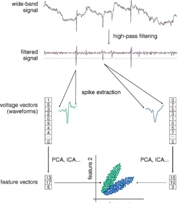
Processing of electrophysiological data requires three steps (Fig. 1). First, putative action potentials (‘spikes’) must be detected and extracted from the wide-band signals in hard-ware or softhard-ware. This is usually done first by high-pass fil-tering and thresholding, then by extracting an adequate num-ber of voltage samples (e.g., corresponding to a time window of a spike) each time a predetermined threshold is crossed. Thus, each spike is described by a vector, the components

(2)

Fig. 1. Processing of electrophysiological spike data. First, wide-band continu-ous brain signals are high-pass filtered and thresholded to detect putative action potentials (‘spikes’); waveforms are extracted around the peak of each spike. Second, the high-dimensionality of the waveforms is reduced for subsequent sorting, using e.g., principal component analysis. Finally, the resulting feature vectors are sorted. The goal of this process is to group the action potentials emit-ted by each single neuron into distinct clusters. Ideally, each recorded action potential is assigned to the neuron that emitted it.

of which are successive voltages in time. The second step is feature extraction. Although complete voltage vectors (‘wave-forms’) are the most accurate description of the spikes, they are rarely appropriate for subsequent processing because of their high dimensionality. There are several methods to drastically reduce the number of components per spike while retaining most of the relevant information. These include principal compo-nent analysis (PCA,Abeles and Goldstein, 1977), independent component analysis (ICA, Jutten and Herault, 1991), factor analysis, and other related methods. The third step is ‘spike sorting’, where spikes are tentatively assigned to the individ-ual neurons that have emitted them. This results in grouping spikes in different ‘clusters’ corresponding to different puta-tive neurons (hence, this process is also referred to as ‘cluster cutting’). Spike sorting is most efficiently performed by com-bining semi-automatic and manual approaches (Harris et al., 2000).

Action potentials of single cells are embedded in networks and related to behavior and the ultimate goal of spike detec-tion is to reveal these reladetec-tionships. Therefore, spikes should be displayed and compared to spikes of other neurons, local field potentials and behavioral events. To facilitate these analyses, we describe a number of computer applications and tools, which allow for processing and visual exploration of the data before subsequent quantitative analyses.

2. The software suite

What makes the package described here different from other existing offerings is threefold. First and foremost, it is free soft-ware distributed under the GNU General Public License (GPL, see http://www.gnu.org/licenses/gpl.html). With this license, our users are explicitly granted legal permission to copy and redistribute the software, as well as to modify it (or have some-one modify it) using the source code. We therefore distribute the software both in binary and source forms (care was taken to develop high-quality, clear and documented code). We hope this will help form a community of interested investigators willing to contribute to the project. The second difference is that our soft-ware can be downloaded from the internet at no cost. The third difference is that because our software was developed within a neuroscience laboratory rather than by an external company, the feature set was directly chosen and defined by experimenters. This resulted in a package with numerous and relevant advanced features (such as the Error Matrix View or the Trace View in Klusters). In addition, constant and direct user feedback ensured that the programs featured easy and efficient user interfaces: intuitive and flexible layout of the graphical elements, numerous configurable keyboard shortcuts and consistent keyboard navi-gation, optimized display speed, highly responsive interface via multithreading, etc.

Our package runs on GNU/Linux and MacOS X and is expected to run on any Unix-like system that includes the KDE libraries and libxml2. We provide installable binary packages for Debian-based distributions (Debian, KNOPPIX, Kubuntu, etc.) and SUSE. Alternatively, the applications can be built from source (they are known to run on e.g., RedHat and MacOS X with Fink). Detailed information is available at the respective websites.

3. Data formats and preprocessing

Contrary to many data acquisition and processing programs, our software does not use a single file with a complex struc-ture, but a collection of very simple files. This ensures that files are easy to read from and write to, and can thus be manipulated using any data analysis package without requir-ing complex import and export filters. There are dedicated files for continuous brain signals (wide-band .dat, local field poten-tials .eeg, high-pass filtered .fil, etc.), spike waveforms (.spk), feature vectors (.fet), spike clusters (.clu), behavioral events (.evt) and position tracking (data file formats are described in Supplementary Figs. 2 and 3). To reduce disk usage, poten-tially large files (continuous brain signals and spike wave-forms) contain multiplexed binary data. All other files contain ASCII format data, making them easy to manipulate by stan-dard Unix file utilities. Files are homogeneous and do not con-tain headers. All the relevant information (number of channels, sampling frequency, spike waveform length, date and com-ments, etc.) is stored in a common parameter file in XML format. This standard, well-supported, self-described format allows for easier extensibility for future versions of the soft-ware.

(3)

L. Hazan et al. / Journal of Neuroscience Methods 155 (2006) 207–216 209

In many cases, data needs preprocessing before analyses can be performed. An example is spike extraction from con-tinuously recorded wide-band signals. Continuous recording of wide-band signals allows for a complete post-hoc replay and exploration of the original, unprocessed brain signals recorded during the experiment. Other examples of data preprocessing include extracting from a video stream the position of the head lights carried by the animal, concatenating multiple recording files, or simply converting data files from a proprietary format to one of our open formats.

4. Klusters: a graphical spike sorting application

Klusters is a graphical application for manual spike sorting. It can be used either to improve the output of automatic clustering or to manually cluster raw data. The initial set of features was inspired by the cluster cutting program sgclust by J. Csicsvari (unpublished).

Klusters works with a spike waveform file (.spk) and a fea-ture file (.fet), and optionnally a cluster file (.clu) produced by an automatic clustering program (Harris et al., 2000) such as KlustaKwik (K.D. Harris,http://klustakwik.sourceforge.net). For data recorded continuously, the wide-band recording file (.dat) can also be used to display raw traces. Once the clusters have been manually created or refined by the experimenter, upon saving a cluster file (.clu) is created.

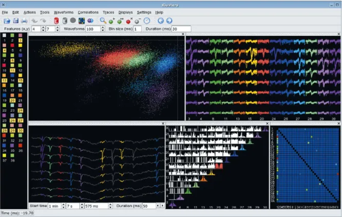
After loading the files, Klusters displays an overview of the data. This includes several graphical elements referred to as ‘views’, namely a cluster view, a waveform view and a cor-relation view (described in detail below). It is possible to work with several displays in parallel, each of which can flexibly com-bine different numbers and types of views arranged in custom layouts and showing different subsets of the data (Fig. 2). On the left side of the main window is the palette where each cluster is represented as a colored square. Clusters selected in the palette are shown simultaneously in all the views of the currently active display. Notice that in order to ensure rapid and easy identifica-tion, individual clusters are drawn using the same customizable colors throughout the application (palette and views).

4.1. Cluster views

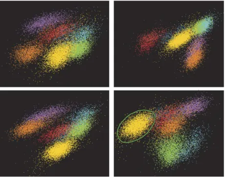
For viewing and editing purposes, Klusters provides clus-ter views displaying two-dimensional projections of the feature vectors. To help visualize the data in multiple dimensions, any number of cluster views can be combined to display different projections simultaneously (Fig. 3). Several editing tools are available. These allow for direct manipulation of whole spike clusters as well as arbitrary subsets of points enclosed within user-defined polygons.

Klusters provides several specific tools to discard ‘artefacts’ and biological signals designated as ‘noise’ (e. g., background small amplitude multiunit activity). Discarded spikes are never actually deleted from the data files; rather, by convention, arte-facts and noise are assigned to clusters 0 and 1, respectively. Klusters provides additional tools to create new clusters or cor-rect existing clusters. Although automatic spike sorting should

ideally yield one distinct cluster for each neuron, in practice, two different kinds of systematic error can occur, which require manual correction: ‘overclustering’, where spikes emitted by a single neuron are split in multiple clusters, and ‘underclus-tering’, where individual clusters contain spikes from multiple neurons. To correct for overclustering, multiple clusters can be grouped together. A special case occurs when one or more elec-trodes drift during the course of the recording session. In this case automatic spike sorting typically splits the spikes in several clusters because spike amplitudes change as a function of time. Selecting time as one of the projection dimensions and carefully inspecting the resulting clusters helps correct for such errors (Fig. 4). To correct for underclustering, one can split existing clusters by manually selecting arbitrary sets of points. These are extracted from their current clusters and, depending on the tool, either grouped together in a single new cluster, or assigned to one new cluster for each original cluster.

4.2. Waveform views

Assessing whether a cluster is contaminated by action poten-tials of other neurons or artefacts, or determining whether two or more clusters actually correspond to a single neuron, is facilitated by inspection and comparison of spike waveforms (Supplementary Fig. 1). Klusters provides waveform views where the waveforms for the currently selected clusters are dis-played as colored traces (side by side, or overlaid). Because clusters can contain hundreds of spikes, by default only a sub-set of the waveforms are actually displayed (in order to reduce display time and memory usage). There are two possible selec-tion modes: the view displays either a user-defined number of waveforms evenly spaced in time, or all waveforms occurring within a customizable time frame. Waveform means and stan-dard deviations can also be displayed.

4.3. Correlation views

Autocorrelograms and cross-correlograms plotted in cor-relation views (Fig. 5) provide invaluable information for assessing the success of spike clustering. For instance, well isolated clusters contain spikes emitted by a single neuron, and thus their autocorrelograms show a clear refractory period (McCormick et al., 1985; Fee et al., 1996; Csicsvari et al., 1998; Harris et al., 2000). Conversely, autocorrelograms which do not show a clear refractory period correspond to ‘noisy’ clusters, i.e. clusters which combine spikes emitted by multiple units. Auto- and cross-correlograms also help finding instances of single neurons erroneously split across multiple clusters (cross-correlograms resembling the respective auto(cross-correlograms) and identifying successive spikes within complex spikes (one-sided cross-correlograms): for example, the asymmetry and common refractoriness of the crosscorrelograms between clusters 11 and 15 are strong indications that these subclusters should be combined since they represent subsequent spikes of complex spike bursts. In addition, the correlation view is also used for screening monosynaptic excitatory and/or inhibitory connec-tions between cell pairs, characterized by short-latency, large

(4)

L. Hazan et al. / Journal of Neur oscience Methods 155 (2006) 207–216

Fig. 2. Klusters. An overview, showing a cluster view (two-dimensional projection of the feature vectors, top left view), a waveform view (top right view), a trace view (spikes highlighted on wide-band brain signals, bottom left view), a correlation view (auto- and crosscorrelograms, bottom middle view), and an error matrix view (color-coded matrix of mean identification error probability, bottom right view). Individual views can be interactively moved around in the display, and more views can be added (e.g., additional cluster views using different projection features, and additional correlation views displaying different time scales). For rapid identification, data from single clusters are represented using the same color throughout the interface, including the selection palette (left panel). Several tools are shown in the tool bar (icons): delete artefact cluster(s) (red trash can), delete noise cluster(s) (grey trash can), update error matrix (colored matrix), group clusters (intersecting purple and blue spheres), zoom (magnifier lens), new cluster (green sphere with a plus sign), split clusters (green sphere with two plus signs), delete artefact spikes (red sphere with a cross sign), delete noisy spikes (grey sphere with a minus sign), select time (clock), previous and next spikes (blue arrows). Several view parameters can be adjusted in the various text fields: projection features, number of waveforms, correlogram bin size and half duration, trace start time and duration (data provided by David Robbe).

(5)

Fig. 3. Cluster views. Each view shows different two-dimensional projections of the feature vectors. Different clusters are represented by different colors. Any number of cluster views can be used simultaneously in order to display different projections of the data side-by-side. Editing tools allow for the creation of new clusters from points enclosed in user-defined polygons (green polygon in lower right panel), as well as grouping or deletion of existing clusters.

Fig. 4. Time axis in cluster views. Using time as one of the projection dimensions shows how spike features change over the course of a recording session. Top: this cluster shows evidence for electrode drift, as indicated by the magnitude shifts of the feature on they-axis. Such drifts may occur when the electrode is located very close to the neuron and even relatively small relative movements can induce noticeable spike waveform changes (e.g., in amplitude). When this happens, the automatic clustering algorithms typically split the spikes across multiple clusters (bottom left), which can misleadingly appear distinct in two-dimensional projections (bottom right). Here, using time as one of the projection dimensions helps identify such misidentification.

amplitude, 1–3 ms wide bins or spike suppression (Csicsvari et al., 1998; Barth´o et al., 2004).

4.4. Error matrix view

Although visual inspection of auto- and crosscorrelogram is necessary for the adjustment of clusters, quantification of such errors is advantageous when large numbers of clusters are formed. To this end, Klusters provides an error matrix view, a graphical representation of a statistical measure of cluster sim-ilarities (Fig. 2). This view indicates for each pair of clusters the mean probability that the spikes in the first cluster actually belong to the second cluster, using the same estimation method as the Classification Expectation Maximization (CEM) algo-rithm (Celeux and Govaert, 1992) implemented in KlustaKwik.

4.5. Trace views

Provided that continuous wide-band signals were recorded during the experiment, Klusters can use the corresponding data file (.dat) to display trace views where brain signals (spikes and local field potentials) are shown in time (Fig. 2). Explor-ing raw data allows for direct assessment of statistical proper-ties evidenced e.g., in auto- and cross-correlograms, and helps detect spurious effects or confirm likely hypotheses (for instance regarding complex spike bursts). Trace views feature a reduced set of the functionalities available in NeuroScope such as spike browsing (see below).

4.6. Automatic reclustering

Although Klusters features a number of tools to correct for underclustering, in most cases manually splitting

(6)

clus-Fig. 5. Correlogram views. Autocorrelograms (colored histograms) and cross-correlograms (white histograms) help determine isolation quality. For instance, cluster 6 has a noisy refractory period, indicating poor isolation. Similar refractory periods in the auto- and the cross-correlograms together with a single-sided peak in the cross-correlograms for clusters 11 and 15 reveal splitting of spikes of bursty neurons. Autocorrelogram 3 with its broad shoulder is indicative of a putative fast spiking interneuron. The asymetric cross-correlogram for clusters 13 and 14 (right) suggests a bidirectional monosynaptic connection between excitatory and inhibitory neurons. Displaying a longer time scale (right vs. left) can reveal firing rythmicity (e.g., for cluster 14). Notice the average firing rate optionally indicated in the color boxes and as dashed horizontal lines.

ters involves arbitrary and potentially biasing choices (a typ-ical example is cluster ‘shaving’, where peripheral points are removed from a cluster). To allow for unbiased reclustering of a set of existing clusters, Klusters can interactively run an auto-matic clustering program on a subset of the data. This is usually a computing intensive task, which can require long processing time, and should thus be performed on a reduced number of clusters. In particular, this feature should not be used as a graph-ical front-end to initial automatic cluster cutting over the whole data. For large files, this can run for up to several days on current computer hardware.

4.7. Exporting as vector graphics

Once optimal clusters have been determined, it is often use-ful to export waveform traces, spike cluster plots and cross-correlograms for presentations or manuscripts. Although this can be achieved by simply using a screen capture utility, doing so results in bitmapped images that do not scale or print well. Instead, Klusters can export high-quality graphics to PostScript (PS) or Portable Document Format (PDF) files. These standard vector graphics formats can then be imported in any drawing application for further editing.

5. Neuroscope: an electrophysiological and behavioral viewer

NeuroScope is a viewer for continuously recorded signals (e.g., wide-band or local field potentials), spiking activity, and behavioral events.

NeuroScope is not a data analysis program; rather, it allows for the easy and efficient inspection of raw data. Although statistical analyses and plots provide synthetic views of data

properties, direct examination of raw data often provides invalu-able insight into the fine structure underlying these properties, helps avoid spurious effects, and may generate hypotheses for subsequent quantitative analyses. NeuroScope was specifically designed to efficiently handle large amounts of data (dozens of channels recorded at high sampling rates, plus dozens of neu-ronal spike trains, and video tracking).

NeuroScope works with a continuous recording file (.dat, .eeg, .fil, etc.). Optionally, it can also display unit activity loaded from spike timings files (.res) and cluster files (.clu), as well as position tracking data from a position file (.whl), and behavioral events from one or more event files (.evt). Although NeuroScope is mainly a viewer application, it features limited editing capa-bilities allowing for modification of event files (.evt), such as adding markers to visually identified events.

NeuroScope displays the data in a trace view (electrophysi-ological signals) and optionally a position view (position track-ing) combined in a display (Fig. 6). Similarly to Klusters, it is possible to work with several displays in parallel, each of which can show different subsets of the data. On the left side of the main window is the palette where channels, units and events are represented as colored icons in dedicated tabbed layouts. Again, rapid and easy identification is ensured by drawing indi-vidual elements using the same customizable colors throughout the application (palette and views).

5.1. Browsing continuous brain signals

Any number of continuously recorded channels can be dis-played in custom colors and arrangements (Fig. 7). Data brows-ing combines direct access to specific points in time, and step-by-step replay of recordings across time. The duration of the data displayed in the view can be adjusted (doubled, halved,

(7)

Fig. 6. NeuroScope. An overview, showing the trace view (electrophysiological signals, bottom view) and a position view (position tracking, here using two head lights, top view). For rapid identification, data from single sources (e.g., channel, cluster) are represented using the same color throughout the interface, including the selection palette (left panel). Several tools are shown in the tool bar (icons): zoom (magnifier lens), draw time line (grey arrow with vertical bar), select channels (blue arrow with horizontal trace), select event (yellow arrow with vertical dashed bar), add event (yellow arrow with vertical dashed bar and plus sign), measure (mutlimeter), select time (clock), previous and next spikes (blue arrows), previous and next events (yellow arrows), move channels to new group (square with four blue spheres and yellow star), remove channels from group (square with four blue spheres and red cross), discard channels (blue trash can), keep channels (blue sphere), skip channels (to label bad channels on silicon probes, crossed blue sphere), show channels (eye), hide channels (crossed eye). Trace start time and duration can be adjusted in the respective text fields.

set explicitly or interactively), for instance to show an overview of brain rhythms over longer periods of time, or help inspect spiking activity over shorter periods of time. A zooming tool is also provided to focus on even more restricted portions of the data (for instance, data sampled from a specific channel during a small time window).

5.2. Browsing unit activity

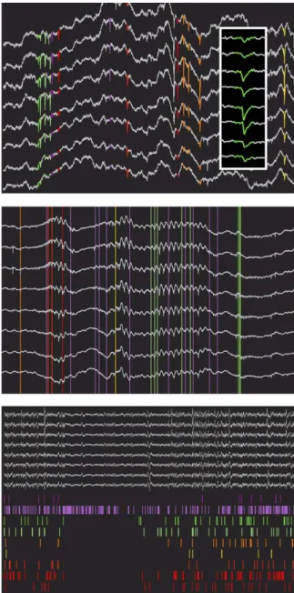
Unit activity can be represented as rasters below the con-tinuous traces, vertical lines spanning the entire view, or full waveforms highlighted directly on the continuous traces (Fig. 8). Rasters allow for inspection of patterns of population activity, vertical lines emphasize relations between unit activity and local field events, and spike highlighting on the traces makes it pos-sible to examine and compare waveforms at higher temporal resolution. For quick and convenient browsing, NeuroScope pro-vides the possibility to directly move to the next or previous spike within a user-defined set of spike trains.

5.3. Position tracking

Provided the position of the animal was tracked during the experiment, NeuroScope can plot successive positions across time (using the same time window as for brain signals), each position being plotted as a connected set of colored points along a regular polygon, one point per head light carried by the animal (Fig. 6). By convention, the front light is plotted in red and all

other lights in green. Thus, if the animal carries a single light, this will be represented as a red dot on the position tracking view, if it carries two lights (required to measure head direction), this will be represented as a segment with a red dot at the front end and a green dot at the back end, etc. To better estimate where the animal is located in the experimental apparatus, it is possible to display in the background an overhead photograph of the maze and/or the trajectory of the animal over the course of the entire experiment.

5.4. Browsing and editing events

Events can be plotted as vertical dashed lines in the trace view, and as cross marks in the position view, at the position occupied by the animal when they occurred (Fig. 6). Similar to spikes, one can directly move to the next or previous event in a user-defined set of events. Although NeuroScope is essentially a viewer, it also features a limited set of editing tools, allowing for addition, deletion and modification of events. This is particularly useful to manually indicate, or correct automatic detection of, field events such as hippocampal ripples, thalamo-cortical spindles, epileptic spikes, etc.

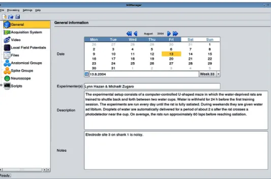
6. NDManager: a simple experimental parameter manager

Klusters and NeuroScope share a common parameter file (this is also used by other tools, as described in the next section). This file stores in XML format all the parameters required for data

(8)

Fig. 7. Trace views: layouts. Electrode groups are displayed in different col-ors, either in vertical arrangements (top, tetrodes), in columnar arrangements (middle, silicon probes with regularly spaced recording sites), or in arbitrary layouts (bottom, epidural electrode array, arranged according to the topography of recording sites).

viewing and processing, including:

• general information: date, experimenter, description, notes;

• acquisition system: number of channels, sampling rate, reso-lution (in bits), offset, voltage range and amplification gain;

• video: sampling rate and frame size;

• file information: sampling rate and channel correspondence for processed files (e.g., low-pass filtered local field poten-tials, high-pass filtered data, average tetrode narrow-band field potentials, etc.)

• anatomical and spike groups: anatomical layout of the elec-trodes and groups for spike extraction and sorting;

• preprocessing parameters: software filter cutoff frequencies, spike extraction threshold, number of samples per waveform, number of principal components, etc.

Fig. 8. Trace views: unit activity. Simultaneous display of clustered unit activity and field recordings. Unit activity can be shown as highlighted spike waveforms directly on the traces (top), emphasizing waveform shapes (inset, lower time scale), as vertical lines overlaid on the traces, emphasizing relations between unit and field activity (middle), or as rastergrams below the traces, emphasizing population firing patterns (bottom).

All these parameters can be edited graphically using NDMan-ager (Fig. 9). This simple application is designed to handle two related tasks: managing experimental parameters edition and data processing execution (as described below).

7. Integrated framework

Klusters, NeuroScope and NDManager are the three main components of a framework intended to provide all the necessary tools to process the data to bring it to suitable form for subse-quent analysis: filtering, spike extraction and sorting, position tracking, event preprocessing, etc. Although several recording systems provide integrated tools to perform these steps, our

(9)

Fig. 9. NDManager. This simple application is designed to handle the parameter file used Klusters and NeuroScope, as well as processing utilities. Parameters are grouped into categories (left panel) and include general information (right panel: date, experimenters, description of the experiment, notes), information about the acquisition system, preprocessing parameters, etc. NDManager is also designed to run preprocessing utilities. Thus, it constitutes a convenient central point from where parameters can be edited, files can be processed, and Klusters and NeuroScope can be started.

package offers a number of advantages: it allows researchers to modify and redistribute it as they see fit (hopefully bring-ing together a community of users and developers constantly improving this common resource); it includes powerful spike sorting capabilities by combining KlustaKwik, an efficient auto-matic clustering program, and Klusters, an advanced manual clustering application (most other packages only offer basic capabilities); it has the capability to eventually include all pro-cessing steps in an integrated suite.

In our framework, non-interactive processing such as high-pass filtering is typically done by command-line tools, usually written in C (but any other language can be used as well to develop additional custom components). Preprocessing does not require user intervention except for the definition of initial parameters (e.g., high-pass threshold). Although for technically sophisticated users, the command-line is a satisfactory user inter-face, for most users a simple graphical interface may be required, if only to define these parameters and start the actual process-ing more easily. This functionality is provided by NDManager, which has the capability to act as a graphical ‘front-end’ to any processing tools. This allows researchers to easily integrate their own processing tools within our framework without code modification. Only an intermediate script is required to read the parameters from the XML file (rather than from the command-line or legacy configuration files), and pass them along to the tools.

In practice, tools are executed via simple scripts (these can be written in sh, bash, perl, python, etc.), which first test the environment to anticipate possible errors (e.g., missing data files required for a specific task), then read parameters from the XML parameter file, and finally generate a command to start the respective tools. Along with each script and tool pair, a

descrip-tion file in XML format describes the parameters required for the task and provides a short help text. NDManager dynami-cally generates a graphical interface from this file, presenting the user a list of named parameters where values can easily be edited. Once all values have been provided, NDManager can execute the script, which reads these values and starts the tool accordingly.

8. Conclusion

The applications presented here allow for advanced process-ing and visualization of neurophysiological data sets includprocess-ing brain signals (action potentials and local field potentials), behav-ioral events and position tracking. These applications can be downloaded from the internet (http://neuroscope.sourceforge. net, http://klusters.sourceforge.net, and http://ndmanager. sourceforge.net). All the applications and tools described here are free software distributed under the GNU General Public License (GPL, seehttp://www.gnu.org/licenses/gpl.html). This license grants its users legal permission to copy, distribute and/or modify the software as they see fit. To this end, the source code is distributed alongside of the executable binaries. The only restriction imposed on the users is that should they decide to redistribute the software in its original or modified form, they must in turn grant their users the same rights. This guarantees that the software or any derivative of it will always remain freely available to the neuroscience community, and avoids the risk of vendor ‘lock in’ associated with proprietary software. We hope to attract an active community of users who could benefit from and contribute to this project.

(10)

Acknowledgements

We wish to thank Jozsef Csisvari, Anton Sirota, Léna¨ıc Mon-conduit, Judith Creso, David Robbe, Stephan Marguet, Sean Montgomery, Derek Buhl, Kenneth Harris, Peter Barthó and Hajime Hirase who helped define the feature set of the appli-cations. Data used in the figures were provided by M. B. Z, Léna¨ıc Monconduit, Anton Sirota, David Robbe, Sean Mont-gomery and Peter Barthó. Supported by National Institutes of Health (NS34994, NS43157, MH54671) and the Human Fron-tier Science Foundation (to M. B. Z).

Appendix A. Supplementary data

Supplementary data associated with this article can be found, in the online version, atdoi:10.1016/j.jneumeth.2006.01.017.

References

Abeles M, Goldstein MH. Multispike train analysis. In: Proceedings of the IEEE, vol. 65; 1977. pp. 762–73.

Barth´o P, Hirase H, Monconduit L, Zugaro M, Harris KD, Buzs´aki G. Characteri-zation of neocortical principal cells and interneurons by network interactions and extracellular features. J Neurophysiol 2004;92:600–8.

Buzs´aki G, Horv´ath Z, Urioste R, Hetke J, Wise K. High-frequency network oscillation in the hippocampus. Science 1992;256:1025–7.

Buzs´aki G. Large-scale recording of neuronal ensembles. Nat Neurosci 2004;7:446–51.

Celeux G, Govaert G. A classification EM algorithm for clustering and two stochastic versions. Computational Statistics Data Anal 1992;14:315–32. Csicsvari J, Hirase H, Czurko A, Buzs´aki G. Reliability and state dependence

of pyramidal cell-interneuron synapses in the hippocampus: an ensemble approach in the behaving rat. Neuron 1998;21:179–89.

Csicsvari J, Henze DA, Jamieson B, Harris KD, Sirota A, Barth´o P, Wise KD, Buzs´aki G. Massively parallel recording of unit and local field potentials with silicon-based electrodes. J Neurophysiol 2003;90: 1314–23.

Eichenbaum HB, Davis JL. Neuronal ensembles: strategies for recording and decoding. New York: Wiley-Liss; 2001.

Fee MS, Mitra PP, Kleinfeld D. Automatic sorting of multiple unit neuronal sig-nals in the presence of anisotropic and non-Gaussian variability. J Neurosci Methods 1996;69:175–88.

Hampson RE, Simeral JD, Deadwyler SA. Distribution of spatial and nonspatial information in dorsal hippocampus. Nature 1999;402:610–4.

Harris KD, Henze DA, Csicsvari J, Hirase H, Buzs´aki G. Accuracy of tetrode spike separation as determined by simultaneous intracellular and extracel-lular measurements. J Neurophysiol 2000;84:401–14.

Hoffman KL, McNaughton BL. Coordinated reactivation of distributed memory traces in primate neocortex. Science 2002;297:2070–3.

Jutten C, Herault J. Blind separation of sources. Part I. An adaptive algorithm based on neuromimetic architecture. Signal Process 1991;24:1–10. Khazipov R, Sirota A, Leinekugel X, Holmes GL, Ben-Ari Y, Buzs´aki G. Early

motor activity drives spindle bursts in the developing somatosensory cortex. Nature 2004;432:758–61.

McCormick DA, Connors BW, Lighthall JW, Prince DA. Comparative electro-physiology of pyramidal and sparsely spiny stellate neurons of the neocortex. J Neurophysiol 1985;54:782–806.

Nicolelis MA. Methods for neural ensemble recordings. Florida: CRC-Press; 1998.

Nicolelis MA, Dimitrov D, Carmena JM, Crist R, Lehew G, Kralik JD, Wise SP. Chronic, multisite, multielectrode recordings in macaque monkeys. Proc Natl Acad Sci USA 2003;100:11041–6.

Wilson MA, McNaughton BL. Dynamics of the hippocampal ensemble code for space. Science 1993;261:1055–8.

Wilson MA, McNaughton BL. Reactivation of hippocampal ensemble memories during sleep. Science 1994;265:676–9.

Zugaro MB, Monconduit L, Buzs´aki G. Spike phase precession persists after transient intrahippocampal perturbation. Nat Neurosci 2005;8:67–71.