A
S
PATIO
-T
EMPORAL
M
ODEL OF
H
OUSE
P
RICES
IN THE
US
S
EAN
H
OLLY
M.
H
ASHEM
P
ESARAN
T
AKASHI
Y
AMAGATA
CES
IFO
W
ORKING
P
APER
N
O
.
1826
CATEGORY 10: EMPIRICAL AND THEORETICAL METHODS
OCTOBER 2006
An electronic version of the paper may be downloaded
• from the SSRN website: www.SSRN.com
• from the RePEc website: www.RePEc.org
CESifo Working Paper No. 1826
A
S
PATIO
-T
EMPORAL
M
ODEL OF
H
OUSE
P
RICES
IN THE
US
Abstract
The purpose of this paper is to apply recent advances in the econometrics of panel data to a problem that has a clear spatial dimension. We model the dynamic adjustment of real house prices using data at the level of US States. In the last decade, in most OECD countries there has been a significant rise in real house prices. This attracted the attention of many international organisations and central banks. In this paper we consider interactions between housing markets by examining the extent to which real house prices at the State level are driven by fundamentals such as real income, as well as by common shocks, and determine the speed of adjustment of house prices to macroeconomic and local disturbances. We take explicit account of both cross sectional dependence and heterogeneity. This allows us to find a cointegrating relationship between house prices and incomes and to identify a small role for real interest rates. Using this model we then examine the role of spatial factors, in particular the effect of contiguous states by use of a weighting matrix. We are able to identify a significant spatial effect, even after controlling for State specific real incomes, and allowing for a number of unobserved common factors.
JEL Code: C21, C23.
Keywords: house price, cross sectional dependence, spatial dependence.
Sean Holly Faculty of Economics Cambridge University Sidgwick Avenue Cambridge, CB3 9DD United Kingdom [email protected] M. Hashem Pesaran Faculty of Economics Cambridge University Sidgwick Avenue Cambridge, CB3 9DD United Kingdom [email protected] Takashi Yamagata Faculty of Economics Cambridge University Sidgwick Avenue Cambridge, CB3 9DD United Kingdom [email protected] 19 September 2006
We would like to thank Ron Smith and Elisa Tosetti for useful comments. Financial support from the ESRC under Grant No. RES-000-23-0135 is gratefully acknowledged.
1
Introduction
The long standing interest of geographers and regional scientists in spatial issues has spelt over into economics and into the development of spatial econometrics (Paelinck and Klaasen, 1979, Anselin, 1988, Krugman 1998) with a particular emphasis placed on inter-actions in space (spatial autocorrelation) and spatial structures (spatial heterogeneity). At the same time there are many economic studies based on panels of economic data at the city, state, regional and country level that have an implicit spatial structure, but which e¤ectively ignore possible spatial interactions and interdependencies. This may not matter if the spatial interactions are captured by common observed factors which are themselves included in the panel model. However, in practice there may be spatial interactions that are not adequately captured in this way.
In the literature on spatial econometrics the degree of cross section dependence is
calibrated by means of a weighting matrix. For example the (i; j) elements of a weighting
matrix,wij, could take a value of 1 if theithandjthareas/regions/countries are contiguous
and zero otherwise1. Of course there are many other forms of contiguity that draw on
the metaphor of a chessboard with the type of connectiveness re‡ecting the scope for movements by the rook, the bishop and the queen. Weights can also be based on distance, squared distance or the number of nearest neighbours. Often, however, in economic applications space may not be the appropriate metric (Conley and Dupor, 2003, and Conley and Topa, 2002 ). In some instances trade ‡ows might be relevant, whilst in the case of inter-industry dependencies input-output matrices might provide the appropriate spatial metric. Alternatively, there may be dependencies between geographical areas that re‡ect cultural similarity, and migration or commuting relationships (E¤, 2004).
Much of these forms of interaction are unobservable, or di¢ cult to measure. We need a method to test for possible hidden interactions. Recently tests have been proposed (Pesaran, 2004) for spatial dependence based on the average of pair-wise correlation coe¢ cients of the OLS residuals from the individual regressions in the panel. Where spa-tial dependence is detected (perhaps due to an unobservable common factor or factors) a widely employed way of taking account of this in modelling is to use a …xed, non-stochastic spatial weights matrix. Another way would be to use (for a su¢ ciently large number of cross section observations) the common correlated e¤ects estimator of Pesaran (2006a). This is a new approach to estimation and inference in panel data models with a multifactor error structure where the unobserved common factors are (possibly) corre-lated with exogenously given individual-speci…c regressors, and the factor loadings di¤er over the cross section units. The basic idea behind the proposed estimation procedure is to …lter the individual-speci…c regressors by means of (weighted) cross-section aggregates
such that asymptotically as the cross-section dimension (N) tends to in…nity the
di¤er-ential e¤ects of unobserved common factors are eliminated. The estimation procedure has the advantage that it can be computed by OLS applied to an auxiliary regression where the observed regressors are augmented by (weighted) cross sectional averages of the dependent variable and the individual speci…c regressors. Two di¤erent but related problems are addressed: one that concerns the coe¢ cients of the individual-speci…c re-gressors, and the other that focuses on the mean of the individual coe¢ cients assumed random. In both cases appropriate estimators, referred to as common correlated e¤ects
(CCE) estimators, are proposed and their asymptotic distribution asN tends to in…nity,
with T (the time-series dimension) …xed or asN and T tend to in…nity (jointly) are
rived under di¤erent regularity conditions. One important feature of the proposed CCE mean group (CCEMG) estimator is its invariance to the (unknown but …xed) number of
unobserved common factors asN and T tend to in…nity (jointly). In this paper we apply
this methodology to an analysis of house prices at the State level in the USA.
Recently there has been considerable interest in the behaviour of house prices not only in the US but also internationally (IMF, 2004). The majority of OECD countries have experienced a considerable rise in real house prices in the last decade. Because of the role housing wealth plays in household behaviour, fears have been expressed that there is a ‘bubble’in house prices, with prices moving well away from their fundamental drivers (Case and Shiller, 2003, McCarthy and Peach, 2004). Changes in real house prices relative to household income can also have important consequences for household budgets, with implications for the design of social policy, and possibly, the behaviour of the macroeconomy. Maclennan, Muellbauer, and Stephens (1998), for example, argue that there are huge di¤erences in housing and …nancial market institutions across Europe and that this has profound e¤ects on the way in which output and in‡ation in the di¤erent countries respond to changes in short-term interest rates, as well as to external shocks to asset-markets. One important aspect of the interaction between the housing market and the macroeconomy arises from the link to the labour market. For example, Bover, Maullbauer and Murphy (1989) argue that di¤erences in the level of house prices between regions lowers labour mobility. See also Meen (2002).
House prices at the regional level also exhibit much more volatility both over time and across regions. Pollakowski and Ray (1997) examine the spatial di¤usion process of the change in the log of US regional house prices, using vector autoregressive (VAR) models. Their results suggest that at the national level (dividing US into nine regions) evidence con…rms the signi…cance of some (non spatial) di¤usion patterns, but at the metropolitan area level there is evidence of contiguous spatial di¤usion.
Recently Cameron et al. (2006) have investigated the evolution of house prices across
nine UK regions between 1972 and 2003. Their model of real house prices is an error correction panel data model with regional e¤ects and time e¤ects, derived from a system of inverted housing demand equations, including additional terms to take into account spatial correlation, as well as supply side e¤ects, credit conditions, etc. Speci…cally, a seemingly unrelated regression (SUR) estimation approach is adopted to control for contemporaneous correlation, and lagged dependent variables of contiguous regions and Greater London are also included to control for the spatial di¤usion process. This esti-mation strategy, apart from its rather complex structure, can not be applied when the number of regions is relatively large, as is the case in the present study.
Housing is typically a largely immovable asset. However, as an asset it is reasonable to assume that at the margin the price of two identical houses located spatially will di¤er only by a (…xed) factor which re‡ects general aspects of physical location. In this paper the fundamental driver of real house prices is real income. However, there is considerable di¤erences among US States in both the level and rates of growth of real
incomes.2 This heterogeneity should in turn be re‡ected in real house prices. We examine
this possibility in the context of a panel error correction model (Malpezzi, 1999, Capozza et al.,2002, and Gallin, 2003). The importance of heterogeneity in spatially distributed housing markets has been highlighted recently by Fratantoni and Schuh (2003). They quantify the importance of spatial heterogeneity in US housing markets for the e¢ cacy of monetary policy. Depending on local conditions monetary policy can have di¤ering
e¤ects on particular US regions (Carlino and DeFina, 1998).
The plan of the paper is as follows. Section 2 discusses the theory underlying house price determination. Section 3 provides a review of the panel data model and estimation methods. Section 4 provides a preliminary data analysis. Section 5 reports the estimation results. Section 6 provides some concluding remarks.
2
Modelling House Prices
It is now standard to see the determination of house prices as the outcome of a market for the services of the housing stock and as an asset. A standard model of the demand for housing services includes permanent income, the real price of housing services and a set of other in‡uences a¤ecting changes in household formation such as demographic shifts.
In equilibrium the real price of houses, Ph=Pg, is equal to the real price of household
services from home ownership, s, divided by the user cost of housing, c:
Ph=Pg =s=c;
where Pg is a general price index. Assume that alternative assets are taxed at the rate
. c is then equal to the expected real, after-tax rate of return on other assets with a
similar degree of risk:
c= (r+ )=(1 ) e; (2.1)
whereris the risk-equivalent real interest rate on alternative assets and e is the expected
rate of price in‡ation. Following the approach of Feldsteinet al. (1978), Hendershott and
Hu (1981) and Buckley and Ermisch (1982), assume that the alternative asset is some aggregate capital which can be …nanced by the issue of equity or the sale of bonds. The bonds are of an equivalent degree of risk to house ownership. Equity is riskier, so there is a market determined risk premium, , on the holding of equity. In equilibrium the risk
adjusted return on equity,", is equal to the return on bonds:
(1 )" = (r+ )=(1 ) e. (2.2) The return to equity is expressed as the dividend payout per unit of equity.
Another way of deriving the user cost of housing is to use the full intertemporal model of consumption in which in equilibrium the marginal rate of substitution between housing services and the ‡ow of utility from consumption is:
uh=uc = (Ph=Pg)f(r+ )=(1 ) e e(Ph=Pg)g; (2.3)
where e(P
h=Pg)denotes the expected appreciation in the real price of houses anduh and
uc are the marginal utilities of housing services and consumption, respectively. The price
of houses that satis…es the market for housing services and the asset market arbitrage condition is then:
Ph=Pg =s=f(r+ )=(1 ) e e(Ph=Pg)g. (2.4)
The empirical model that can be derived from this form of analysis employs the device
of proxying the unobservable real rental price of the ‡ow of housing services, s, by the
3
The Econometric Model and Tests
The long-run relation compatible with the theory can be written most conveniently in the following log-linear form:
pit = i+ 0ixit+uit; i= 1;2; :::; N;t = 1;2; :::; T; (3.1)
where pit = log(Pit;h=Pit;g) is the logarithm of real price of housing in the ith State,
xit = (yit; rlit)0, yit is real personal disposable income in the ith State, and rlit is the logarithm of real interest rate. The price dynamics and their adjustments to the long-run
equilibrium across States are captured in the error terms uit. The common unobserved
factors as well as the spatial e¤ects will also be modelled through the error terms. In
particular, we shall assume thatuit has the following multi-factor structure
uit = 0ift+"it; (3.2)
in which ft is an m 1 vector of unobserved common e¤ects, and "it are the
individual-speci…c (idiosyncratic) errors assumed to be distributed independently ofxitandft.
How-ever, we allow"0
itsto be weakly dependent acrossi. This, for example, allows the
idiosyn-cratic errors to follow the Spatial Autoregressive (SAR), or the Spatial Moving Average (SMA) processes introduced by Whittle (1954), Cli¤ and Ord (1973, 1981), and Haining (1978).
Despite its simplicity the above speci…cation is reasonably general and ‡exible and allows us to consider a number of di¤erent factors that drive house prices. Some of the supply factors that are particularly di¢ cult to measure accurately can be captured
through the unobserved common components of uit.3 The speci…cation also allows for
the possible e¤ects of the transmission of monetary policy onto house prices at the aggre-gate level. We are also able to test for cointegration between real house prices and real disposable income, whilst allowing for a high degree of dependence across States.
3.1
The Common Correlated E¤ects (CCE) Estimator
We use the Common Correlated E¤ects (CCE) type estimator, which asymptotically
eliminates the cross dependence (Pesaran 2006a). To illustrate, suppose the (k 1)
vector xit is generated as
xit =ai+ 0ift+vit; (3.3)
where ai is a k 1 vector of individual e¤ects, i is a m k factor loading matrices
with …xed components, vit are the speci…c components of xit distributed independently
of the common e¤ects and across i; but assumed to follow general covariance stationary
processes. Combining (3.1) and (3.3) we now have
zit (k+1) 1 = pit xit = di (k+1) 1 + C0i (k+1) m ft m 1 + it (k+1) 1 ; (3.4)
3The supply elasticity of housing units has recently been identi…ed as an important factor behind
house price movements in some US urban markets. The ease with which regulatory approval for the construction of new houses can be obtained has been identifed by Glaeser and Gyourno (2005) and Glaeser, Gyourko and Saks (2005) as a signi…cant element in real house price increases in California, Massachusetts, New Hampshire, New Jersey and Washington, DC.
where it = "it+ 0ivit vit ; (3.5) di = 1 0i 0 Ik i ai , Ci = i i 1 0 i Ik ; (3.6)
Ik is an identity matrix of order k, and the rank of Ci is determined by the rank of the
m (k+ 1) matrix of the unobserved factor loadings
~i =
i i : (3.7)
Pesaran (2006a) has suggested using cross section averages of pit and xit as proxies for
the unobserved factors in (3.1). To see why such an approach could work, consider simple
cross section averages of the equations in (3.4)4
zt=d+C0ft+ t; (3.8) where zt= 1 N N X i=1 zit, t = 1 N N X i=1 it; and d= 1 N N X i=1 di, C= 1 N N X i=1 Ci. (3.9) Suppose that
Rank(C) =m k+ 1, for all N: (3.10)
Then, we have ft = CC0 1 C zt d t : (3.11) But since t q:m: ! 0, as N ! 1, for each t; (3.12) and C!p C= ~ 1 0 Ik ; asN ! 1; (3.13) where ~ = (E( i); E( i)) = ( ; ): (3.14)
It follows, assuming that Rank(~) = m, that
ft (CC0)
1
C zt d p
!0, asN ! 1:
This suggests using (1;z0
t)0 as observable proxies for ft, and is the basic insight that lies
behind the Common Correlated E¤ects (CCE) estimators developed in Pesaran (2006a).
Kapetanios et al. (2006) prove that the CCE estimators are consistent regardless of
whether the common factors,ft, are stationary or nonstationary. It is further shown that
the CCE estimation procedure in fact holds even if ~ turns out to be rank de…cient, thus
the estimator is consistent with any …xed number of m. This contrasts to the principal
4Pesaran (2006a) considers cross section weighted averages that are more general. However, we used
component approach, which requires us to estimate the number of factors (Bai and Ng, 2002, and Bai, 2003).
The CCEMG estimator is a simple average of the individual CCE estimators, ^bi of
i de…ned by ^ bM G =N 1 N X i=1 ^ bi; (3.15) ^ bi = (X0iMXi) 1X0iMpi; (3.16)
where Xi = (xi1;xi2; :::;xiT)0,pi = (pi1; pi2; :::; piT)0, and M is de…ned by
M=IT H H0H
1
H0; (3.17)
andH= ( T;Z), T is a (T 1) vector of unity,Zis aT (k+ 1)matrix of observations
zt. The (non-parametric) variance estimator for b^M G is given by
d V ar ^bM G = 1 N(N 1) N X i=1 ^ bi ^bM G ^bi ^bM G 0 .
E¢ ciency gains from pooling of observations over the cross section units can be
achieved when the individual slope coe¢ cients, i, are the same. Such a pooled
esti-mator of , denoted by CCEP, has been developed by Pesaran (2006a) and is given
by ^ bP = N X i=1 X0iMXi ! 1 N X i=1 X0iMpi: (3.18)
The variance estimator for ^bP is given by
d V ar b^P =N 1^ 1R ^^ 1; (3.19) where ^ =N 1 N X i=1 X0 iMXi T ; (3.20) ^ R = 1 N 1 N X i=1 X0iMXi T ^ bi b^M G b^i b^M G 0 X0iMXi T : (3.21)
3.2
A Cross-Section Dependence Test
In this paper we use a CD (Cross-section Dependence) test of error cross dependence,
which does not require ana priori speci…cation of a connection (weighting) matrix and is
applicable to a variety of panel data models, including stationary and unit root dynamic
heterogeneous panels with structural breaks, with short T and large N (Pesaran, 2004).
The CD test is based on an average of the pair-wise correlations of the OLS residuals from the individual regressions in the panel, and tends to a standard normal distribution
as N ! 1. The CD test statistic is de…ned as
CD = s 2T N(N 1) NX1 i=1 N X j=i+1 ^ij ! a sN(0;1); (3.22)
where^ij is the sample estimate of the pair-wise correlation of the residuals. Speci…cally, ^ij = ^ji = PT t=1u^itu^jt PT t=1u^ 2 it 1=2 P T t=1u^ 2 jt 1=2; (3.23)
where u^it is the OLS estimate of uit de…ned by
^
uit =pit ^i ^
0
ixit; (3.24)
with ^i and ^i being the estimates of i and i computed using the OLS regression of
pit on an intercept and the regressors, xit;for each i;separately.
3.3
Panel Unit Root Tests
One of the most commonly used tests for unit roots in panels is that of Im, Pesaran and
Shin (2003), called the IPS test. Consider a pth order Augmented Dickey-Fuller (ADF)
regression for theith cross section unit:
!it =ai+ it+bi!i;t 1+
p
X
j=1
ij !i;t j + it; i= 1;2; :::; N, t= 1;2; :::; T: (3.25)
The unit root hypothesis of interest can be expressed as
H0 :bi = 0 for all i, against the possibly heterogeneous stationary alternatives,
H1 :bi <0, i= 1;2; :::; N1,bi = 0, i=N1+ 1; N1+ 2; :::; N.
It is assumed thatN1=N is non-zero and tends to a …xed constant such that0< 1
as N ! 1, which is necessary for the consistency of the panel unit root test. The
individual pth order ADF statistic, ADF(p), is obtained as the OLS t-ratio of bi, ^t
i, and
the IPS statistic is de…ned as5
IP S = p N t-bar E ^tijbi = 0; p q V ar ^tijbi = 0; p ; (3.26) where t-bar=N 1 N X i=1 ^ ti. (3.27)
The values of E ^tijbi = 0; p and V ar ^tijbi = 0; p with various combinations of T and
p are tabulated in Im, Pesaran and Shin (2003). Under the null hypothesis, the
distrib-ution of the IP S statistic is well approximated by the standard normal distribution for
su¢ ciently large N and T.
However, the IPS test procedure is not valid when the errors, it, are dependent
across i, and its use in the case of the house price data can lead to spurious inference. A
number of panel unit root tests that allow for possible cross section dependence in panels 5The dependence of the statistics onN and/orT are suppressed for ease of notation.
have been recently proposed in the literature.6 Here we consider two of these that are
particularly relevant to our application. One is the test proposed by Moon and Perron (2004) which is based on the t-ratio of a modi…ed pooled OLS estimator using the de-factored panel data. For de-factoring, they make use of principal components estimator of
mcommon factors, where the number of factorsmis estimated using the model selection
criteria proposed in Bai and Ng (2002). In their paper two test statistics, ta and tb, are
proposed. Here only the latter is considered, which was reported to have better …nite sample performance in Moon and Perron (2004). Following Moon and Perron (2004) the long-run variances are estimated using Andrews and Monahan (1992) estimator based on
a quadratic spectral kernel and prewhitening. Under the null, the statistic tb tends to a
standard normal variate as both N and T go to in…nity so long as N=T !0.
The second panel unit root test considered in our application is the test proposed by Pesaran (2006b), which follows the CCE approach and …lters out the cross section dependence by augmenting the ADF regressions with cross section averages. The cross section augmented ADF (CADF) regressions, carried out separately for each State, are given by !it =ai+ it+bi!i;t 1+ci!t 1+ p X j=0 dij !t j + p X j=1 ij !i;t j+vit; (3.28)
where !t denotes the cross section mean of !it. The CIPS statistic is a simple cross
section average of ~ti de…ned by
CIP S=N 1 N X i=1 ~ ti; (3.29)
where ~ti is the OLS t-ratio of bi in the above CADF regression. Pesaran (2006b) also
considers a truncated version of t~i so that these statistics have …nite moments even for
relatively small N and/or T. The truncated version of the CIPS statistic is de…ned as
CIP S =N 1PN
i=1t~i, wheret~i are truncated CADF statistics such that
8 < : ~ ti = ~ti; if K1 <t~i < K2; ~ ti = K1; if ~ti K1, ~ ti =K2; if ~ti K2,
K1 and K2 are positive constants that are su¢ ciently large so thatPr K1 <~ti < K2
is su¢ ciently large. The choice of the value ofK1 andK2 depends on the speci…cation of
CADF 0s. For models with an intercept only, K1 = 6:19 and K2 = 2:61, and for models
with an intercept and a linear trend, K1 = 6:42 and K2 = 1:70, are used. The critical
values for the CIPS tests are given in Tables 2a-2c in Pesaran (2006b).7
3.4
Cointegration between Real House Prices and Real Incomes
Recently there has been a debate in the literature about whether there is cointegration between real house prices and real per capita disposable incomes. In the absence of cointegration there is no fundamentals driving real house prices so the possibility of bubbles is increased (Case and Shiller, 2003). So far the evidence is mixed.
6For a recent surevy of the literature see Breitung and Pesaran (2006).
Malpezzi (1999) uses panel data on 133 metropolitan areas in the US over 18 years from 1979 to 1996 and applies the panel unit root test of Levin, Lin and Chu (2002, LLC) to house price-to-income ratios, and …nds that he can not reject the presence of a unit root in these series. But he is able to reject the null of a unit root in the residuals of the regressions of real house prices on real per capita incomes, again using the LLC panel
unit root test.8 However, the testing procedure adopted by Malpezzi su¤ers from two
main shortcomings. The LLC’s critical values are not appropriate when the panel unit root test is applied to residuals from …rst step regressions, and perhaps more importantly, the LLC test does not take account of possible cross section dependence of house prices and this could seriously bias the test results.
Capozza, et al. (2002) recognize this problem and try to control for cross section
dependence by adding time dummies to their error correction speci…cations. However, as Gallin (2003) points out, local housing market shocks are likely to be correlated in ways that are not captured by simple time e¤ects. To allow for more general error cross section dependence, Gallin (2003) adopts a bootstrap version of Pedroni’s (1999) residual-based cointegration test procedure, and concludes that ".. even these more powerful tests do not reject the hypothesis of no cointegration." However, the bootstrap approach, originally advanced in Maddala and Wu (1999), is likely to be seriously biased. The bootstrap test statistic is not pivotal, and the bootstrap test has a …nite sample error of the same order as the asymptotic test. Secondly, as Maddala and Wu (1999) show, the bootstrap procedure cannot eliminate size distortions in …nite samples, particularly in cases where
N is small relative to T. Also see Smith, Leybourne, Kim and Newbold (2004,
p.161-168) where they …nd that the bootstrap panel unit root test tends to under-reject when
N =T = 25. They do not consider any experiments where N > T. Furthermore, their
Monte Carlo set up does not deal with common factor error structures, since it ensures that the maximum eigenvalue of the error variance-covariance matrix remains bounded
in N, by design.9 In Gallin’s application N (= 95) is much larger than T (= 23), and
due to the presence of common factors the N N error variance-covariance matrix is
likely to be near singular. The bootstrap panel unit root tests reported by Gallin can be subject to large size distortions.
Over the past few years a number of panel cointegration tests have been proposed in the literature that attempt to take account of error cross section dependence in their test procedures. These include the tests proposed by Groen and Kleibergen (2003), Nelson, Ogaki, and Sul (2005),Westerlund (2005), Pedroni and Vogelsang, (2005), Chang (2005), and Bai and Kao (2006). The tests by Groen and Kleibergen, Nelson, Ogaki,
and Sul, and Westerlund are applicable when N is small and T large. For example,
in their Monte Carlo experiments Groen and Kleibergen and Nelson, Ogaki, and Sul
consider panels with N 8 and T 100. Westerlund considers panels where N = 10
or at most 20 and T = 50 or 100. The tests by Pedroni and Vogelsang and Chang, in
principle, can deal with panels where N is reasonably large, but their models do not
allow for unobserved common factors, ft, that could be correlated with the observed
regressors, xit, which is an important consideration in our application. When ft and
8It is not clear if the panel unit root tests reported in Malpezzi are applied to the levels of
price-to-income ratios or to their logarithms. See equation (2) and the discussions on pages 42 and 48 in Malpezzi (1999).
9See, for example, Chamberlain and Rothschild (1983) who show that in the case of factor models
in N variables and a …xed number of factors m, the largest eigenvalue of the covariance matrix of the variables must rise withN.
xit are correlated the …rst stage residuals used in the tests by Chang and Pedroni and Vogelsang will be inconsistent which invalidates their residual-based testing procedures. Bai and Kao model cross section dependence using the factor approach as in (3.2), but assume that the innovations to the factors and the observed regressors are independently distributed. (see their Assumption 2). However, as Bai and Kao note in their Remark 1, it
is possible to relax their Assumption 2 by allowing the innovations inxit to be correlated
with ft. For a more detailed review of this emerging literature see, for example, Breitung and Pesaran (2006).
We follow Chang, Pedroni and Vogelsang, and Bai and Kao and adopt a two-stage
procedure to assess the possibility of cointegration between the log of real house price (pit)
and the log of real per capita disposable income (yit). But unlike these studies, in both
stages we allow for unobserved common factors that could be potentially correlated with the observed regressors. Using the pooled CCE estimator we …rst estimate the residuals,
^
uit = pit ^CCEyit ^i. As noted earlier, the pooled estimate, ^CCE is consistent for
, under fairly general assumptions about the unobserved common factors, ft. We then
apply panel unit root tests to these residuals. If the presence of a unit root inu^it’s can be
rejected we shall conclude that the log of real house prices and the log of real per capita
disposable incomes are cointegrated with the cointegrating vector given by (1; ^CCE)0.
4
Preliminary Data Analysis
We begin our empirical investigation with a preliminary analysis of spatial dependence at the US State level, using data on the growth of real house prices and incomes. Table 1 de…nes the variables used. A more detailed description is provided in the Data Appendix. We use annual data on US States, excluding Alaska and Hawaii, from 1975 to 2003. One of the features of the data in which we are interested, is the extent to which real house prices are driven by fundamentals such as income. To explore spatial interactions we calculate simple correlation coe¢ cients between each State, within and between correlations for the Bureau of Economic Analysis (BEA) eight regions and …nally the within and between correlation coe¢ cients for three geographical regions dividing the USA into broadly the West, the Middle and the East. The results are shown in Tables 3 and 4.
In Table 3 we tabulate within and between correlation coe¢ cients for the 8 BEA regions. The diagonal elements show the within region average correlation coe¢ cient. The o¤ diagonal elements give the between region correlation coe¢ cients. For many regions the within region correlation is larger than the between region correlation. But for some regions this is not so. For example, the States of the Mideast region are more correlated on average with the States of New England than among themselves. The States of the Great Lakes are more correlated with those of the South East than they are among themselves. If we look at the correlations at the level of 3 geographical areas, the within correlations are always larger than the between, though the East tends to be ‘closer’in some sense to the Middle than the Middle is to the West. Overall, real income growth is correlated across the USA.
In Tables 4 we tabulate the spatial correlations for real house prices. A similar picture to that for real incomes emerges. Within region correlations are generally larger than the between correlations, with the exception of New England and the Middle East and the South West and the Rocky Mountains. In contrast to the results for real incomes there is a more noticeable spatial pattern. The growth of real house prices in New England is
hardly correlated at all with States in the Rocky Mountains and the Far West, with the correlations on average declining with distance. This pattern is also clear when we look at the three broad geographical areas (The West, the Middle and the East).
The regional groupings also disguise some interesting correlations at the underlying State level. To save space, the State level correlation coe¢ cients for real income growth and real house price growth are not included in this paper, but are available upon re-quest. Real income growth in California is more closely correlated with many States that are geographically very distant. This re‡ects the common factors driving economic development in di¤erent parts of the USA, such as the growth of aerospace, information technology etc. that stimulate growth in di¤erent States. For real house prices the av-erage correlation coe¢ cient between States is 0.39 compared to 0.51 for real incomes. There are also some unusual correlations at the individual State level. Real house price growth in California, for example, is more closely correlated with Washington DC and Maryland (0.86 and 0.73 respectively) than with New York (0.16) or Oregon (0.25).
Overall, there is more evidence in the raw data of a possible spatial pattern in real house prices than in real incomes, but there are also a number of between State correla-tions that appear to be independent of spatial patterns.
5
Econometric Evidence
In this section we turn to the test and estimation results.
5.1
Panel Unit Root Tests Results
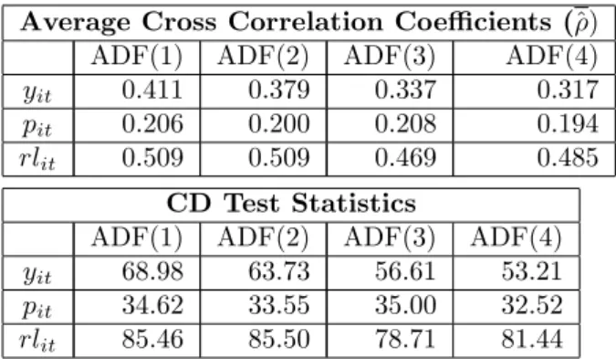
The extent of cross section dependence of the residuals from ADF(p) regressions of real
house prices, real incomes and interest rates across the 49 States over the period 1975 to
2003 are summarized in Table 5. For eachp= 1;2;3and 4we computed average sample
estimates of the pair-wise correlations of the residuals, which we denote by^. To capture
the trended nature of real incomes and real house prices we run the ADF regressions with linear trends, but included an intercept only in the regressions for real interest rates. The
results are reasonably robust to the choice of the augmentation order,p. For real incomes
and real interest rates, ^is estimated to be around40% and50%, respectively, whilst for
real house prices it is much lower and the estimate stands at 20%. This largely re‡ects
the national character of changes in incomes and interest rates as compared to real house prices that are likely to be a¤ected by State speci…c e¤ects as well. The results are also in line with the pair-wise correlations of the raw data discussed above and con…rm the existence of a greater degree of cross State correlations in the case of real incomes as compared to real house prices.
The CD test statistics, also reported in Table 5, clearly show that the cross correlations are statistically highly signi…cant, and thus invalidate the use of panel unit root tests, such the IPS test, that do not allow for error cross section dependence. Therefore, in
what follows we shall focus on the Moon-Perron’s tb and Pesaran’s CIP S tests.
The results for Moon and Perrons’stb test are summarized in Table 6. The application
of the tb test requires an estimate of m, the number of common factors. We tried the
various selection criteria proposed in Bai and Ng (2002), all of which require starting from
an assumed maximum value of m; denoted by mmax. But the outcomes did not prove
to be satisfactory, in the sense that the choice of m often coincided with the assumed
results for various values of m in the range of 1 to 4. For changes in real incomes and
real house prices the tb test rejects the unit root hypothesis, but for the levels of these
variables the test results depend on whether linear trends are included or not. In the case of house prices the test outcomes also depend on the assumed number of factors. Only for real interest rates do the test results convincingly reject the unit root hypothesis.
The CIPS test results, summarized in Table 7, show a similar outcome for the real
interest rates. But for pit and yit the unit root hypothesis can not be rejected if the
trended nature of these variables are taken into account. This conclusion seems robust to the choice of the augmentation order of the underlying CADF regressions. As the Moon
and Perron test is valid only when T is much larger than N, we believe the CIPS test
results are more reliable for our data. We proceed taking yit and pit asI(1), and rlit as
I(0) variables.
5.2
The Income Elasticity of Real House Prices
To test for a possible cointegration between pit and yit, we …rst estimate the following
fairly general model
pit = i+ iyit+uit, i= 1;2; :::; N; t= 1;2; :::; T, (5.1) where uit = m X `=1 i`f`t+"it. (5.2) In view of discussion in Section 3, the common correlated e¤ects (CCE) estimators are
consistent regardless of f`t being stationary or non-stationary, so long as "it is stationary
and m is a …nite …xed number (See Pesaran, 2006a, Kapetanios et al., 2006). To show
the importance of allowing for the unobserved common factors in this relationship we
also provide naive estimates of i, i = 1;2; :::; N (and their mean) that do not allow for
cross section dependence by simply running OLS regressions of pit on yit. The common
correlated e¤ects (CCE) estimators are based on the cross section augmented regressions
pit = i+ iyit+gi0yt+gi1pt+eit, (5.3)
where yt and pt denote the cross section averages ofyit and pit in yeart. The results are
reported in Table 8. The …rst column gives the naive mean group estimates. These suggest a small coe¢ cient on income of only 0.30, and considerable cross sectional dependence. The other two columns report the common correlated e¤ects mean group (CCEMG) and the common correlated e¤ects pooled (CCEP) estimates. The coe¢ cient on income is now signi…cantly larger and the residual cross sectional dependence has been purged with
the average correlation coe¢ cient, ^, reduced from 0.38 for the MG estimates to 0.024
and 0.003 respectively for the CCEMG and CCEP estimates.
The CCEMG and CCEP estimates and their standard errors also support the hypoth-esis of a unit elasticity between changes in house prices and real incomes. The t-ratios
of both CCE estimates in Table 8 are less than unity for the null hypothesis of interest.
Therefore, the long-run relation to be tested for cointegration is given by
^
uit =pit yit ^i, where ^i =T 1PtT=1(pit yit).
5.3
Panel Cointegration Test Results
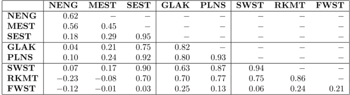
The residuals u^it can now be used to test for cointegration between pit and yit. Note
that the CCE estimates are consistent irrespective of whether ft are I(0), I(1) and/or
cointegrated. The presence offt also requires that the panel unit root tests applied tou^it
should allow for the cross section dependence of the residuals. The extent to which these residuals are cross-sectionally dependent can be seen from the average cross correlation
coe¢ cients ofu^it, within and between the eight BEA regions,which are reported in Table
9.
We computed CIPS(p) panel unit root test statistics forpit yit, including an intercept,
for di¤erent augmentation and lag orders, p = 1;2;3 and 4, and obtained the results,
2:16; 2:39; 2:45;and 2:29, respectively. The 5%and 1% critical values of the CIPS
statistic for the intercept case and panels withN = 50 and T = 30 are 2:11and 2:23,
respectively. The results suggest rejection of a unit root inpit yitfor all the augmentation
orders at5% level and rejection at 1%level in the case of the augmentation orders2 and
more.
5.4
Panel Error Correction Speci…cations
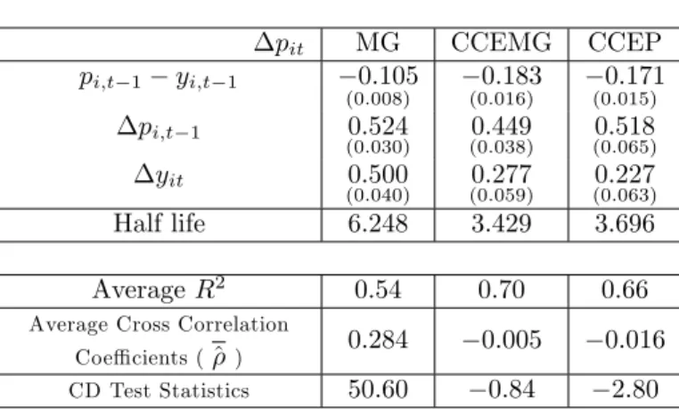
Having established panel cointegration between pit and yit, we now turn our attention
to the dynamics of the adjustment of real house prices to real incomes and estimate the panel error correction model:
pit = i+ i(pi;t 1 yi;t 1) + 1i pi;t 1+ 2i yit+ it: (5.4)
The coe¢ cient i provides a measure of the speed of adjustment of house prices to a
shock. The half life of a shock to pit is approximately ln(2)=ln(1 + i).
To allow for possible cross section dependence in the errors, it, we computed CCEMG
and CCEP estimators of the parameters, as well as the mean group (MG) estimators that do not take account of cross section dependence. The former estimates as computed by OLS regressions of piton1;(pi;t 1 yi;t 1), pi;t 1, yit, and the associated cross section
averages,(pt 1 yt 1), yt, pt, and pt 1. The results are summarized in Table 10. The
coe¢ cients are all correctly signed. The CCEMG and CCEP estimators are very close
and yields error correction coe¢ cients ( 0:183 and 0:171) that are reasonably large
and statistically highly signi…cant. The average half life estimates are around 3.5 years, much smaller than the half life estimates of 6.3 years obtained using the MG estimators. But the MG estimators are likely to be biased, since the residuals from these estimates show a high degree of cross sectional dependence. The same is not true of the CCE type estimators.
To check for the e¤ect of real interest rates on real house prices we also estimated
the above ECM with rli;t 1 included. (see Table 11).10 We found a small negative e¤ect
from real interest rates on real house prices, but the e¤ect was not statistically signi…cant
at the conventional levels. This could partly be due to the fact that rli;t 1 is de…ned in
terms of a common nominal rate of interest and the cross section variations of rli;t 1 is
limited to the di¤erences of the lagged in‡ation rates across the States.11 A cross country
analysis of house prices might be needed for a more reliable estimate of the e¤ects of real 10Since the cross section variations ofrl
i;t 1 is due solely to the cross section variations of pi;t 1,
cross section averages of rli;t 1 are not included in the panel regressions. 11We also tried contemporaneous values ofrl
interest rates on real house prices, as such a study is likely to yield a much higher degree of cross section variations in real interest rates.
5.5
Factor Loading Estimates across States
We have shown that the common correlated e¤ects estimators are quite successful in taking out the cross sectional dependence by the use of a multifactor error structure where the unobserved common factors are proxied by …ltering the individual-speci…c regressors
with cross-section aggregates. However, the sensitivity of the ith unit, in this case a
State, to the factors will vary so the factor loadings di¤er over the cross section units. We can obtain an idea of these di¤erential factor loadings if we regress the cointegrating
relationship (pit yit) on (pt yt) and a constant. These regressions are reminiscent of
the Capital Asset Pricing Models (CAPM) in …nance where individual asset returns are regressed on market (or average) returns.
The results, summarized in Table 12, show an interesting pattern in the loadings on the
factor(pt yt). The States are ordered by the BEA’s regions. By construction, the cross
section average of the estimated coe¢ cients on (pt yt) is unity, and the cross section
average of the intercepts is zero. New England and the Mid-East States all have loadings of less than one, while all of the South East States, with the exception of Virginia, have loadings greater than one on the common factor. This is also true for the States in the Plains region and the South West region. The Far West region States all have loadings less than 1 also. But strikingly, there are a number of States that have a zero, or even a negative loading - Massachusetts, Rhode Island, Connecticut, Rhode Island, New Jersey, New York, California, Oregon and Washington. In the case of Massachusetts, New York, and California the loadings are negative, sizeable and statistically signi…cant. These are all States that in the last 25 years have been particular bene…ciaries of new technologies. These innovations interacting with restrictions on new building, have resulted in real house prices deviating from the average across US States.
5.6
Testing for Spatial Autocorrelation
The previous analysis provided consistent estimates of the cointegrating relationship be-tween real house prices and real incomes. In this section we turn to the estimation of spatial patterns based on the estimation of a spatial weighting matrix that is commonly
used in the literature. We investigate the error structure (5.2), based onu^it =pit yit ^i.
We want to distinguish between a common dependence which is captured by the common
factors in (5.2) and idiosyncratic components in "it. These idiosyncratic factors re‡ect
forms of local dependence that are spatial in nature. Initially we applied all six infor-mation criteria (IC) for the estiinfor-mation of the number of factors proposed by Bai and Ng (2002), with the maximum number of factors varied between 1 to 8. Similar to the results in Table 7, all the criteria suggested the same maximum number of factors. In view of
this, we analysedu^it, instead, by principal components form= 1;2 and 3(following Bai
(2003, p.140), for example) so that
^ uit = m X `=1 ~i`f~`t+ ~"it, (5.5)
where f~`t, ` = 1;2; ::; m are the extracted factors and ~i` are the associated factor
regressions of u^it on the estimated factors over the period 1975 to 2003 for eachi. To investigate the strength of spatial dependence in the idiosyncratic components, for
eachmwe estimated the following standard spatial lag model in~"it (Cli¤ and Ord, 1973)
~ "it= N X j=1 wij~"jt + it, (5.6)
where is a spatial autoregressive parameter, andwij is the generic element of theN N
spatial weight matrixW, and it iidN(0; 2). The log-likelihood function of this model
is given by L_ (N T 2 ) ln( 2) +Tln jIN Wj 1 2 2 T X t=1 (~"t W~"t)0(~"t W~"t);
where ~"t = (~"1t;~"2t; :::;"~N t)0, and in our application N = 49 and T = 29.12 For W,
following the approach of Anselin, we used a contiguity criterion and assigned wij = 1
when State i and j share a common border or vertex, and wij = 0 otherwise.13 The
ML estimates of together with their standard errors given in brackets for m = 1;2
and 3are 0.653 (0.022), 0.487 (0.027) and 0.298 (0.033), respectively.14 All the estimates
are highly signi…cant and as is to be expected, the magnitude of the spatial parameter declines markedly with the number of factors. Nevertheless, even with 3 factors there is strong evidence that local dependence in the form of a spatial dependence between contiguous states in the US is present in the data.
We also checked the spatial estimates to see if they are robust to possible di¤erences in the error variances across the States, by estimating the spatial model using standard residuals de…ned by "it = ~"it=si, where si =
p T
t=1~" 2
it=T. We obtained slightly larger
estimates for , namely 0.673 (0.021), 0.513 (0.027) and 0.393 (0.030), for m= 1;2; and
3, respectively. These estimates con…rm a highly signi…cant and economically important
spatial dependence in real house prices in the US, even after controlling for State speci…c real incomes, and allowing for a number of unobserved common factors.
6
Concluding Remarks
This paper has considered the determination of real house prices in a panel made up of 49 US States over 29 years, where there is a signi…cant spatial dimension. An error correction model with a cointegrating relationship between real house prices and real incomes is found once we take proper account of both heterogeneity and cross sectional dependence. We do this using recently proposed estimators that use a multifactor error structure. This approach has proved useful for modelling spatial interactions that re‡ect both geographical proximity and unobservable common factors. We also provide estimates of spatial autocorrelation conditional on up to 3 common factors and …nd signi…cant evidence of spatial dependence associated with contiguity.
12For computation details of maximum likelihood estimation, see Anselinet al. (2006) and references
therein.
13The data on contiguity are obtained from Luc Anselin’s web site at:
http://sal.uiuc.edu/weights/index.html.
14We also computed generalised method of moments estimates proposed by Kelejian and Prucha (1999).
These yielded very similar results to the maximum likelihood estimates. We are grateful to Elisa Tosetti for carrying out the computations of the spatial estimates.
Overall, our results support the hypothesis that real house prices have been rising in line with fundamentals (real incomes), and there seems little evidence of house price bubbles at the national level. But we also …nd a number of outlier States: California, New York, Massachusetts, and to a lesser extent Connecticut, Rhode Island, Oregon and Washington State, with their log house price income ratios either unrelated to the national average or even moving in the opposite direction. It is interesting that these are the States that over the past 25 years have been pioneer and major bene…ciaries of technological innovations in media, entertainment, …nance, and computers.
References
Andrews, D. and Monahan, C., (1992). An improved heteroskedasticity and
autocorre-lation consistent covariance matrix estimator. Econometrica, 60, 953-966.
Anselin, L., (1988). Spatial Econometrics: Methods and Models, Boston: Kluwer
Acad-emic Publishers.
Anselin, L., (2001). Spatial econometrics. In Baltagi, B. (Ed.), A Companion to
Theo-retical Econometrics, Oxford: Blackwell.
Anselin, L., Le Gallo, J. and Jayet, H., (2006). Spatial panel econometrics. In Matyas,
L. and Sevestre, P. (Eds.), The Econometrics of Panel Data, Fundamentals and Recent
Developments in Theory and Practice, (3rd Edition), Dordrecht, Kluwer, forthcoming.
Bai, J., (2003). Inferential theory for factor models of large dimensions. Econometrica,
71, 135-173.
Bai, J. and Kao, C., (2006). On the estimation and inference of panel cointegration model
with cross-sectional dependence. In: Baltagi, B., (Ed.), Panel Data Econometrics:
The-oretical Contributions and Empirical Applications (Contributions to Economic Analysis, Volume 274). Elsevier.
Bai, J. and Ng, S., (2002). Determining the number of factors in approximate factor
models. Econometrica, 70, 161-221.
Bover, O., Muellbauer, J. and Murphy, A., (1989). Housing, wages and the UK labour
market. Oxford Bulletin of Economics and Statistics, 51, 97-136.
Breitung, J. and Pesaran, M.H., (2006). Unit roots and cointegration in panels.
Forth-coming in Matyas, L. and Sevestre, P. (Eds.), The Econometrics of Panel Data (Third
Edition), Kluwer Academic Publishers.
Buckley, R. and Ermisch, J., (1982). Government policy and house prices in the United
Kingdom: An economic analysis. Oxford Bulletin of Economics and Statistics, 44,
273-304.
Cameron, G., Muellbauer, J. and Murphy, A., (2006). Was there a British house price bubble?: Evidence from a regional panel. Mimeo, University of Oxford.
Capozza, D.R., Hendershott, P.H., Mack, C. and Mayer, C.J., (2002). Determinants of
real house price dynamics. NBER Working Paper, 9262.
Carlino, G. and DeFina, R., (1998). The di¤erential regional e¤ects of monetary policy. Review of Economics and Statistics, 80, 9001-9921.
Case, K.E. and Shiller, R. (2003). Is there a bubble in the housing market? Brookings
Chamberlain G., Rothschild M. (1983). Arbitrage, Factor Structure and Mean-variance
Analysis in Large Asset Market, Econometrica, 51, 1305-1324.
Chang, Y., (2005). Residual based tests for cointegration in dependent panels, mimeo, Rice University.
Cli¤, A. and Ord, J.K., (1973). Spatial Autocorrelation, London: Pion.
Cli¤, A. and Ord, J.K., (1981). Spatial Processes, Models and Applications, London:
Pion.
Conley, T.G. and Dupor, B., (2003). A spatial analysis of sectoral complementarity. Journal of Political Economy, 111, 311-352.
Conley, T.G. and Topa, G., (2002). Socio-economic distance and spatial patterns in
unemployment. Journal of Applied Econometrics, 17, 303 - 327.
E¤, E.A., (2004). Spatial, cultural and ecological autocorrelation in U.S. regional data. Working Paper, Middle Tennessee State University.
Feldstein, M., Green, J. and Sheshinksi, E., (1978). In‡ation and taxes in a growing
economy with debt and equity …nance. Journal of Political Economy, 86, 53-70.
Fratantoni, M. and Schuh, S., (2003). Monetary policy, housing investment, and
hetero-geneous regional markets. Journal of Money, Credit and Banking, 35, 557–589.
Gallin, J., (2003). The long run relationship between house prices and income: evidence from local housing markets. Federal Reserve Board.
Glaeser, E.L. and Gyourko, J., (2005). Urban decline and durable housing. Journal of
Political Economy, 113, 345-375.
Glaeser, E.L., Gyourko, J. and Saks, R.E., (2005). Urban growth and housing supply. Harvard Institute of Economic Research, Discussion Paper Number 2062.
Green, R. K. and S. Malpezzi, (2003). A Primer on U.S. Housing Markets and Housing Policy. AREUEA Monograph, Urban Institute Press: Washington.
Groen, J.J.J. and Kleibergen, F., (2003). Likelihood-based cointegration analysis in
panels of vector error-correction models. Journal of Business & Economic Statistics, 21,
295-318.
Haining, R.P. (1978). The moving average model for spatial interaction. Transactions of
the Institute of British Geographers, 3, 202-225.
Hendershott, P.H. and Hu, S.C., (1981). In‡ation and extraordinary returns on
owner-occupied housing: some implications for capital allocation and productivity growth.
Jour-nal of Macroeconomics, 3, 177-203.
Im, K., Pesaran, H. and Shin, Y., (2003). Testing for unit roots in heterogeneous panels. Journal of Econometrics, 115, 53-74.
International Monetary Fund (2004). The global house price boom. World Economic
Outlook, September.
Kapetanios, G., Pesaran, M.H. and Yamagata, T., (2006). Panels with nonstationary
multifactor error structures. Cambridge Working Papers in Economics 0651, University
of Cambridge.
Kelejian, H.H. and Prucha, I.R., (1999). A generalized moments estimator for the
au-toregressive parameter in a spatial model.International Economic Review, 40, 509-533.
Krugman, O., (1998). Space: the …nal frontier. Journal of Economic Perspectives, 12,
161-174.
Levin, A., Lin, F. and Chu, C., (2002). Unit root tests in panel data: Asymptotic and
…nite-sample properties. Journal of Econometrics, 108, 1-24.
Maclennan, D, Muellbauer, J. and Stephens, M., (1998). Asymmetries in housing and
…nancial market institutions and EMU.The Oxford Review of Economic Policy, 14, 54-80.
Maddala, G.S. and Wu, S., (1999). A comparative study of unit root tests with panel
data and a new simple test. Oxford Bulletin of Economics and Statistics, Special Issue,
631-652.
Malpezzi, S., (1999). A simple error correction model of house prices. Journal of Housing
Economics, 8, 27-62.
McCarthy, J. and Peach, R.W., (2004). Are home prices the next “bubble”? Economic
Policy Review, 10, Federal Reserve Board of New York.
Meen, G., (2002). The time-series behavior of house prices: A transatlantic divide? Journal of Housing Economics, 11, 1-23.
Moon, H.R. and Perron, B., (2004). Testing for a unit root in panels with dynamic
factors. Journal of Econometrics, 122, 81-126.
Moran, P.A.P. (1948). The interpretation of statistical maps. Journal of the Royal
Statistical Society, Series B 37, 243-51.
Paelinck, J.H.P and Klaasen, L.H., (1979). Spatial Econometrics, Saxon House.
Nelson, M., Ogaki, M. and Sul, D., (2005). Dynamic seemingly unrelated cointegrating
Pedroni, P., (1999). Critical values for cointegration tests in heterogeneous panels with
multiple regressors, Oxford Bulletin of Economics and Statistics, 61, 653-670.
Pedroni, P. and Vogelsang, T., (2005). Robust unit root and cointegration rank tests for panels and large systems. mimeo, Williams College.
Pesaran, M.H., (2004). General diagnostic tests for cross section dependence in panels. CESifo Working Papers, No.1233.
Pesaran, M.H., (2006a). Estimation and inference in large heterogeneous panels with a
multifactor error structure.Econometrica, 74, 967-1012.
Pesaran, M.H., (2006b). A simple panel unit root test in the presence of cross section dependence. mimeo, University of Cambridge.
Pollakowski, H.O. and Ray, R.S., (1997). Housing price di¤usion patterns at di¤erent
aggregation levels: An examination of housing market e¢ ciency. Journal of Housing
Research, 8, 107-124.
Smith, L.V., Leybourne, S., Kim, T. and Newbold, P., (2004). More powerful panel data
unit root tests with an application to mean reversion in real exchange rates. Journal of
Applied Econometrics, 19, 147-170.
Westerlund, J., (2005). New simple tests for panel cointegration. Econometric Reviews,
24, 297-316.
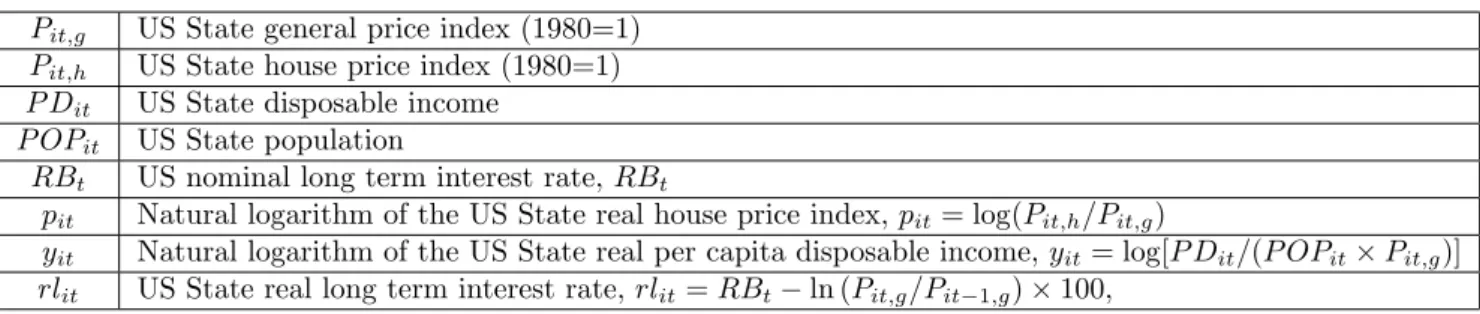
Table 1: List of Variables and their Descriptions
Pit;g US State general price index (1980=1)
Pit;h US State house price index (1980=1)
P Dit US State disposable income
P OPit US State population
RBt US nominal long term interest rate, RBt
pit Natural logarithm of the US State real house price index, pit= log(Pit;h=Pit;g)
yit Natural logarithm of the US State real per capita disposable income, yit= log[P Dit=(P OPit Pit;g)]
rlit US State real long term interest rate, rlit=RBt ln (Pit;g=Pit 1;g) 100;
Notes: Annual data between 1975 and 2003 (T = 29) for 48 States and the District of Columbia. (N= 49). See the Data Appendix for the data sources and a detailed description of the construction of the US State general price index.
Table 2: Regions and Abbreviations
East Middle West
Regions/States Abbrev. Regions/States Abbrev. Regions/States Abbrev.
New England Region NENG Great Lakes Region GLAK Southwest Region SWST Connecticut CT Illinois IL Arizona AZ Maine ME Indiana IN New Mexico NM Massachusetts MA Michigan MI Oklahoma OK New Hampshire NH Ohio OH Texas TX Rhode Island RI Wisconsin WI
Vermont VT Rocky Mountain Region RKMT Plains Region PLNS Colorado CO Mideast Region MEST Iowa IA Idaho ID
Delaware DE Kansas KS Montana MT District of Columbia DC Minnesota MN Utah UT Maryland MD Missouri MO Wyoming WY New Jersey NJ Nebraska NE
New York NY North Dakota ND Far West Region FWST Pennsylvania PA South Dakota SD Alaska AK
California CA Southeast Region SEST Hawaii HI
Alabama AL Nevada NV Arkansas AR Oregon OR Florida FL Washington WA Georgia GA Kentucky KY Louisiana LA Mississippi MS North Carolina NC South Carolina SC Tennessee TN Virginia VA West Virginia WV
Table 3: Average of Correlation Coe¢ cients Within and Between Regions First Di¤erence of Log of Real Per Capita Real Disposable Income (i) Three Geographical Regions
East Middle West East 0:55
Middle 0:51 0:64
West 0:46 0:49 0:48
(ii) Eight BEA Regions
NENG MEST SEST GLAK PLNS SWST RKMT FWST NENG 0:74 MEST 0:58 0:57 SEST 0:48 0:50 0:61 GLAK 0:54 0:56 0:70 0:85 PLNS 0:33 0:34 0:50 0:59 0:61 SWST 0:38 0:46 0:54 0:60 0:46 0:45 RKMT 0:24 0:38 0:44 0:51 0:39 0:49 0:48 FWST 0:51 0:51 0:56 0:66 0:44 0:50 0:41 0:68
Notes: See Table 2 for the regions and abbreviations. The …gures are average of sample pair-wise correlation coe¢ cients.
Table 4: Average of Correlation Coe¢ cients Within and Between Regions First Di¤erence of Log of Real House Prices
(i) Three Geographical Regions East Middle West East 0:48
Middle 0:42 0:65
West 0:19 0:45 0:50
(ii) Eight BEA Regions
NENG MEST SEST GLAK PLNS SWST RKMT FWST NENG 0:80 MEST 0:68 0:66 SEST 0:40 0:32 0:52 GLAK 0:40 0:35 0:57 0:81 PLNS 0:27 0:20 0:53 0:62 0:61 SWST 0:07 0:05 0:35 0:28 0:39 0:52 RKMT 0:03 0:11 0:40 0:52 0:53 0:57 0:70 FWST 0:13 0:17 0:29 0:52 0:42 0:31 0:46 0:57
Table 5: Residual Cross Correlation of ADF(p)Regressions Average Cross Correlation Coe¢ cients (^)
ADF(1) ADF(2) ADF(3) ADF(4)
yit 0:411 0:379 0:337 0:317
pit 0:206 0:200 0:208 0:194
rlit 0:509 0:509 0:469 0:485
CD Test Statistics
ADF(1) ADF(2) ADF(3) ADF(4)
yit 68:98 63:73 56:61 53:21
pit 34:62 33:55 35:00 32:52
rlit 85:46 85:50 78:71 81:44
Notes:pth-order Augmented Dickey-Fuller test statistics, ADF(p), fory
it,pitandrlitare computed for each cross section
unit separately. Foryit and pit, an intercept and a linear time trend are included in the ADF(p) regressions, but for
rlit only an intercept is included. The values in ‘Average Cross Correlation Coe¢ cients’ are the simple average of the
pair-wise cross section correlation coe¢ cients of the ADF(p) regression residuals. ^ = [2=N(N 1)]PNi=11PNj=i+1^ij
with ^ij being the correlation coe¢ cient of the ADF(p) regression residuals between ith and jth cross section units.
CD = p2T =N(N 1)PNi=11PNj=i+1^ij, which tends to N(0;1) under the null hypothesis of no error cross section
dependence.
Table 6: Moon and Perrontb Panel Unit Root Test Results
m 1 2 3 4
With an intercept only
yit 21:90 24:27 29:67 27:85
pit 14:51 15:34 15:03 14:13
yit 6:85 3:29 4:57 3:73
pit 1:06 0:15 0:73 0:03
rlit 10:22 9:39 9:56 8:39
With a Linear Trend
yit 2:49 1:92 5:39 8:35
pit 0:48 2:17 4:28 5:00
Notes: Thetb test is the Moon and Perron (2004) panel unit root test statistic. Thetb statistic is computed for a given number of factors,m= 1;2;3;4. The long-run variances are estimated using the Andrews and Monahan (1992) estimator, using a quadratic spectral kernel and prewhitening. Under the null, thetbstatistic tends to a standard normal distribution as both N andT go to in…nity such that N=T !0. The 5% critical value (one-sided) is -1.645. The superscript “*” signi…es the test is signi…cant at the …ve per cent level.
Table 7: Pesaran’s CIPS Panel Unit Root Test Results
With an Intercept
CADF(1) CADF(2) CADF(3) CADF(4)
yit 2:61 2:39 2:42 2:34
pit 2:28 1:86 1:76 1:81
yit 2:52 2:44 2:39 2:49
pit 2:56 2:44 2:83 2:84
rlit 3:53 2:69 2:05 1:87
With an Intercept and a Linear Trend CADF(1) CADF(2) CADF(3) CADF(4)
yit 2:51 2:22 2:24 2:09
pit 2:18 2:02 2:27 2:30
Notes: The reported values are CIPS(p) statistics, which are cross section averages of Cross-sectionally Augmented Dickey-Fuller (CADF(p)) test statistics (Pesaran 2006b); see Section 3 for more details. The relevant lower 5 per cent critical values for the CIPS statistics are -2.11 with an intercept case, and -2.62 with an intercept and a linear trend case. The superscript “*” signi…es the test is signi…cant at the …ve per cent level.
Table 8: Estimation Result: Income Elasticity of Real House Price MG CCEMG CCEP ^ 3:85 (0:20) (00:26):11 0:00 (0:24) ^ 0:30 (0:09) (01::1420) (01::2021)
Average Cross Correlation
Coe¢ cient ^ 0:38 0:024 0:003 CD Test Statistic 71:03 4:45 0:62
Notes: Estimated model ispit = i+ iyit+uit. MG stands for Mean Group estimates. CCEMG and CCEP signify
the Cross Correlated E¤ects Mean Group and Pooled estimates, respectively. ^ = N 1PN
i=1^i for all estimates, and ^ =N 1PN
i=1^ifor MG and CCEMG estimates. Standard errors are given in parenthesis; see Section 3 for more details.
The ‘Average Cross Correlation Coe¢ cient’ is computed as the simple average of the pair-wise cross section correlation coe¢ cients of the regression residuals, namely^ = [2=N(N 1)]PNi=11PNj=i+1^ij;with^ijbeing the correlation coe¢ cient
of the regression residuals of theiandj cross section units. The CD test statistic is[T N(N 1)=2]1=2 ^, which tends to
N(0;1)under the null hypothesis of no error cross section dependence.
Table 9: Average Residual Cross Correlation Coe¢ cients Within and Between Eight BEA Geographical Regions -u^it=pit yit ^i,
NENG MEST SEST GLAK PLNS SWST RKMT FWST NENG 0:62 MEST 0:56 0:45 SEST 0:18 0:29 0:95 GLAK 0:04 0:21 0:75 0:82 PLNS 0:10 0:24 0:92 0:80 0:93 SWST 0:07 0:17 0:90 0:63 0:87 0:94 RKMT 0:23 0:08 0:70 0:70 0:77 0:75 0:86 FWST 0:12 0:01 0:03 0:25 0:13 0:06 0:24 0:21
Table 10: Panel Error Correction Estimates without Long-Term Interest Rate
pit MG CCEMG CCEP pi;t 1 yi;t 1 0:105 (0:008) 0:183 (0:016) 0:171 (0:015) pi;t 1 0:524 (0:030) (00::449038) (00::518065) yit 0:500 (0:040) (00::277059) (00::227063) Half life 6:248 3:429 3:696 AverageR2 0:54 0:70 0:66
Average Cross Correlation
Coe¢ cients (^ ) 0:284 0:005 0:016 CD Test Statistics 50:60 0:84 2:80
Notes: The State speci…c intercepts are estimated but not reported. MG stands for Mean Group estimates. CCEMG and CCEP signify the Cross Correlated E¤ects Mean Group and Pooled estimates, respectively. Standard errors are given in parenthesis. The AverageR2 is computed as1 PN
i=1^ 2 i= PN i=1^ 2 pi, where ^ 2
i are estimated error variances and^2pi
are sample variances of pit, for each Statei. The half life of a shock topitis approximated by ln(2)=ln(1 + ^)where^
is the pooled estimates for the coe¢ cient onpi;t 1 yi;t 1. Also see the notes to Table 8.
Table 11: Panel Error Correction Estimates with Long-Term Interest Rate
pit MG CCEMG CCEP pi;t 1 yi;t 1 0:114 (0:009) 0:212 (0:016) 0:174 (0:017) pi;t 1 0:494 (0:031) (00::390041) (00::518069) yit 0:536 (0:046) (00::244063) (00::236057) rli;t 1 0:0004 (0:0006) (00::0008)0014 (00::0007)0012 Half Life 5:727 3:072 3:626 AverageR2 0:54 0:72 0:66
Average Cross Correlation
Coe¢ cients (^) 0:291 0:005 0:011 CD Test Statistics 51:94 0:87 1:93
See the notes to Table 10. Since the cross section variations ofrli;t 1is due solely to the cross section variations of pi;t 1
(already included in the model), cross section averages of rli;t 1 were not included in the regressions for the CCE type
Table 12: Factor Loading Estimates (pit yit) (pt yt) Constant Connecticut 0:35 (0:23) 1:42 Maine 0:29 (0:15) 1:90 Massachusetts 0:63 (0:24) 3:99 New Hampshire 0:81 (0:22) 0:51 Rhode Island 0:11 (0:24) 2:76 Vermont 0:78 (0:15) 0:67 Delaware 0:32 (0:11) 1:63 District of Columbia 0:54 (0:18) 0:82 Maryland 0:62 (0:10) 0:81 New Jersey 0:04 (0:20) 2:37 New York 0:39 (0:20) 3:35 Pennsylvania 0:65 (0:13) 0:88 Alabama 1:72 (0:09) 1:54 Arkansas 1:77 (0:10) 1:70 Florida 1:44 (0:08) 1:09 Georgia 1:43 (0:08) 0:89 Kentucky 1:21 (0:06) 0:35 Louisiana 2:03 (0:15) 2:45 Mississippi 2:09 (0:13) 2:33 North Carolina 1:28 (0:05) 0:50 South Carolina 1:39 (0:06) 0:73 Tennessee 1:53 (0:08) 1:14 Virginia 0:91 (0:09) 0:22 West Virginia 2:08 (0:11) 2:47 Illinois 0:71 (0:11) 0:61 Indiana 1:14 (0:05) 0:33 Michigan 0:54 (0:17) 1:01 Ohio 1:01 (0:09) 0:08 Wisconsin 0:98 (0:12) 0:01 Iowa 1:55 (0:11) 1:38 Kansas 1:76 (0:06) 1:90 Minnesota 1:20 (0:09) 0:59 Missouri 1:37 (0:04) 0:90 Nebraska 1:57 (0:10) 1:41 North Dakota 2:00 (0:15) 2:44 South Dakota 1:39 (0:08) 0:90 Arizona 1:02 (0:07) 0:08 New Mexico 0:95 (0:12) 0:23 Oklahoma 2:10 (0:17) 2:70 Texas 2:12 (0:18) 2:77 Colorado 0:80 (0:17) 0:34 Idaho 1:19 (0:11) 0:39 Montana 0:75 (0:16) 0:63 Utah 0:68 (0:19) 0:85 Wyoming 1:62 (0:18) 1:73 California 0:64 (0:23) 3:70 Nevada 0:84 (0:11) 0:16 Oregon 0:37 (0:25) 1:40 Washington 0:12 (0:17) 2:51
Notes: Standard errors are given in parentheses. By construction, the cross section average of the estimated coe¢ cients on(pt yt)is unity, and the cross section average of the intercepts is zero. The negative slope estimates are in bold, and statistically signi…cant slopes are denoted by .
A
Data Appendix
The data set are annual data 1975-2003 and cover 48 States (excluding Alaska and Hawaii), plus the District of Columbia. The US State level house price index (Pit;h) are obtained from the O¢ ce of
Federal Housing Enterprise Oversight. The US State level data of disposable income (P Dit) and the
State population (P OPit) are obtained from the Bureau of Economic Analysis. When only the quarterly
data are available, annual simple averages of the four quarters are used.
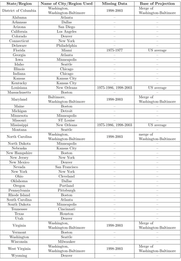
As there is no US State level consumer price index (CPI), we constructed State level general price index, Pit;g, based on the CPIs of the cities/areas. The reasoning is summarized in Table A1. Brie‡y,
we choose the large cities/area of the State or next to the State which have their own CPIs, which are available from the Bureau of Labor Statistics (BLS). Note that this procedure allows multiple States to share a common price index. When the State price index have missing data, they are replaced with the US CPI average or the average of Washington-Baltimore, according to their locations.
The long term interest rate,RBt, which are simple annual averages of quarterly data, are taken from