Spoken Word Recognition Using MFCC and
Learning Vector Quantization
Esmeralda C. Djamal
*, Neneng Nurhamidah and Ridwan Ilyas
Jurusan InformatikaUniversitas Jenderal Achmad Yani Jl. Terusan Jenderal Sudirman, Cimahi *[email protected]
Abstract— Identification of spoken word(s) can be used to
control external device. This research was result word identification in speech using Mel-Frequency Cepstrum Coefficients (MFCC) and Learning Vector Quantization (LVQ). The output of system operated the computer in certain genre song appropriate with the identified word. Identification was divided into three classes contain words such as "Klasik", "Dangdut" and "Pop", which are used to playing three types of accordingly songs. The voice signal is extracted by using MFCC and then identified using LVQ. The training and test set were obtained from six subjects and 10 times trial of the words "Klasik", "Dangdut" and "Pop" separately. Then the recorded sound signal is pre-processed using Histogram Equalization, DC Removal and Pre-emphasize to reduce noise from the sound signal, and then extracted using MFCC. The frequency spectrum generated from MFCC was identified using LVQ after passing through the training process first. Accuracy of the testing results is 92% for identification of training sets while testing new data recorded using different SNR obtained an accuracy of 46%. However, the test results of new data recorded using the same SNR with training data has an accuracy of 75.5%.
Keywords—Spoken word Recognition; MFCC; LVQ; Histogram Equalization; voice command
I. INTRODUCTION
The recognition and classification of sound waves is a difficult problem, which, due to its importance in various domains, receives a lot of attention. Generally, it is determined by three factors: speaker, speech, and emotion expression recognition. Speaker recognition is a biometric authentication process. Speech classification related to phonetic, linguistic, psychological, and computer science that have different perspectives of each so that needs a mediating role that lexical representations and processes play in language understanding, linking sound with meaning. Speech classification often called voice command. However, present methods have been able to improve accuracy. Speech Recognition is more innovative and active area of research for last many years. Beside, emotion expression can be recognized in voice.
Automatic speech recognition systems identify the spoken word(s) represented as an acoustic signal. They have several applications in health care, the military, telephony, and other domains. They can be very helpful for speakers with defect such as dysarthria [1], paraplegia [2], and other muscle disability.
They can be used to improve Kinect software [3], turn on home appliances [4], identify gender [5], analyze infant cry [6].
In the spoken word recognition, the acoustic signal must be extracted before pass machine learning. Previous research used Mel-Frequency Cepstrum Coefficients (MFCC) [1], [7], [8], [9], [10], [11], [12], [13], [4]. Meanwhile another research used Linear Predictive Coding (LPC) [4], [14], and wavelet [15]. Another research compared MFCC more accurate than LPC with accuracy up to 100% [16], [17] and also more accurate than Dynamic Time Warping (DTW) with average 96% [18].
MFCC is popular because the efficient extraction method with its robustness in presence of different noises. In MFCC stage, the speech signal is passed through several triangular filters which are spaced linearly in a perceptual Mel scale. The Mel filter bank log energy (MFLE) of each filters are calculated. Output of MFCC is cepstral coefficients that are computed using linear transformation of MFLE. Although using of a linear transformation on MFCC somewhat problematic for non-linear signal. However, this method remains popular. This weakness is one of them making a small segment span so close to linear, such frame blocking. In noisy conditions, the MFCC-based system provides a relatively strong performance compared to the LPCC, at 20dB SNR level MFCC-based system has an accuracy rate of 97% [19].
In the meanwhile, there are several previous researches in speech recognition usually using Learning Vector Quantization (LVQ) [4], [14], [20], [17] to identify Arabic phonetic [21], Radial Basis Function neural network [9], Support Vector Machine, k Nearest Neighbor [13], Hidden Markov model (HMM) [22], Multilayer Perceptron [19], minimum Euclidean distance [23], power spectrum [5], and Gaussian Mixture Models (GMM) [24], [25].
LVQ is adapted of Self Organizing Kohenen Map with supervised Learning. The advantage of this method lies in the speed of computing considering the revision of weighting performed only for the class winner. Beside voice recognition LVQ used to Brain Computer Interface Game and EEG processing [26], [27].
This research proposed spoken word recognition during two seconds using MFCC and LVQ. Word identifications of three classes are “Klasik”, “Dangdut” and “Pop”, in Indonesian
language. Output of identification system to control song with appropriate genre. Spoken of each subject had passed pre-processing: Histogram Equalization, DC Removal dan Pre– Emphasize filters to normalize and to reduce noise. Then it was extracted using MFCC before had been identified using LVQ. The system was developed with 6 subjects and 10 trial of each word. We got 180 data training and 180 data testing.
II. MATERIAL AND METHODS
A. Data Acquisition
Speech retrieval was performed offline with the three words that are "Klasik", "Dangdut" and "Pop". Each word is associated to the class that will play the song with the appropriate genre. These words have different pronunciation and vowel ending. They was recorded using microphone with SNR larger than 10dB, 8000 Hz sampling frequency, mono channel, and 8-bit resolution.
Each recording has taken two seconds of six subjects and 10 trials. Each recording the subject should speak word “Klasik”, “Dangdut”, and “Pop” (in Indonesian). There are 6 subjects x 10 trials x 3 classes = 180 data set. The subjects was asked to speak with clear articulation and nearly 2 seconds. It means not too fast or to slow so that get good training data. Each recording gave 16000 sampling.
B. Design of Identification System
System identification was developed illustrated by Fig 1.
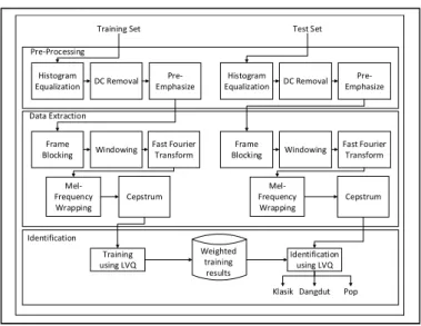
Fig. 1. Design of spoken word identification
Input of the system, which are the speech of six subjects, recorded using microphone with sampling frequency 8000 Hz and 8-bit resolution and mono channel. The sound signal were passed pre-process through three stages, namely Histogram Equalization, DC Removal and Pre-Emphasize filter.
Histogram equalization aims to smooth the amount of sample data to 16000 samples for each recording. The DC Removal process is performed to remove DC components in order to obtain normalization of the sound input data. The
Pre-Emphasize aims to maintain high frequencies on the spectrum and denoising.
After pre-processing, the signal is extracted using MFCC. MFCC consist five stages: Frame Blocking, Windowing, Fast Fourier Transform (FFT), Mel–Frequency Wrapping and Cepstrum. Frame Blocking divide the signal into short segments or short frames to overcome non-stationer as voice signal. Two seconds of signal was segmented into 0.02 seconds, so we obtained 198 frames. Windowing reduced discontinuity of signal in Frame Blocking process. In this research Hamming Window is used because sidelobe is not too high. FFT converted the signal into frequency domain and next process in frequency. Mel-Frequency Wrapping was obtained through Mel-Filterbank. It has signal in triangular window shape, 32 filters, resulting 34 point each frame. Cepstrum is the opposite of the spectrum. It is intended to obtain the information contained in the voice signal, in this study we are using 13 MFCC coefficients of each frame.
The training and identification process is conducted using LVQ. Training process generalize the training data so can be used the other data to identification. If the sound signal generated 13 coefficients of Cepstrum each frame so that one recording produced 13 x 198 framed = 2574 Ceptrum as vectors input for LVQ training. This research classify three classes, namely “Klasik”, “Dangdut” and “Pop” (in Indonesian language).
C. Pre-Processing
The sound signals obtained from the recording have different data widths. It is due to the spoken word of the subject that have varying signal lengths. Therefore, Histogram Equalization was used by calculating the cumulative distribution of the sample data using Eq. 1.
= [ ] + [ − 1] (1)
After obtaining cumulative distribution value, computing of Histogram average or mean of Histogram. They have 16000 data using Eq. 2.
ℎ[ ] = (( [ ]( ) ) ∙ ) + 1 (2) Therefore, the DC Removal process is performed to calculate value - average of the sample data and then subtract out the sound of each data sample to obtain normalization of voice input data by Eq 3.
[ ] = [ ] −∑ [ ] (3)
Previous research has recognized speech signal after pre-processed using DC Removal and remove DC component so we obtained 87% accuracy of random tester [28].
To eliminate noise of sound signal, the Pre-Emphasize filter process was used to maintain high frequencies. It generally eliminated during the sound production process which using Eq. 4, and α is 0.97. [ ] = [ ] − [ − 1] (4) Training Set Pre-Processing Histogram Equalization DC Removal Pre-Emphasize Data Extraction Frame Blocking Windowing Fast Fourier Transform Mel-Frequency Wrapping Cepstrum Identification Training using LVQ Weighted training results Histogram Equalization DC Removal Pre-Emphasize Frame Blocking Windowing Fast Fourier Transform Cepstrum Identification using LVQ
Klasik Dangdut Pop
Test Set
Mel-Frequency Wrapping
D. Mel-Frequency Cepstrum Coefficients
There are five stages in the extraction process using MFCC. Those are: Frame Blocking, Windowing, FFT, Mel-Frequency Wrapping and Cepstrum.
The Frame Blocking process is used to divide the audio signal into the frames. Frame size determination usually using "the power of two". But, the other way is using a zero layer to close the rule of "the power of two". There are sampling time (Ts) every 20ms is due to the signal characteristics changing over a period of time to reflect different sounds on the order of 0.2 seconds or more. Using Equation 5 got 99 frames / second.
( ) + 1 (5) with = ∶ = = 8000 = = 8000 0,02 = 160 = 2 = 160 2 = 80 =8000 − 160 80 + 1 = 99
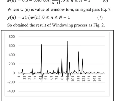
Using Windowing to minimize the signal discontinuities using Eq. 6.
( ) = 0,5 − 0,46 cos , 0 ≤ ≤ − 1 (6)
Where w (n) is value of window to-n, so signal pass Eq. 7.
( ) = ( ) ( ), 0 ≤ ≤ − 1 (7)
So obtained the result of Windowing process as Fig. 2.
Fig. 2. Windowing
FFT converted each N point each frame from time domain to frequency domain. The width of FFT was 160 of length of frame.
Mel-Frequency Wrapping is produced from Mel-Filterbank consisting of a series Triangular Window with overlap. Mel values are not influenced by the logarithmic base choice, given the scale of Mel using natural or decimal logarithms.
There are variations in filter triangular number i.e. 12, 22, 32 and 42. However, too little or too many filters that are used would not provide high accuracy. As previous study, 32 filters
in the extraction using the MFCC gave high accuracy of 85% [23].
The number of filters used were 32, which means Mel-Filterbank has a triangular window as many as 32 pieces with 34 points. The lower limit and the upper limit is determined Mel value between 0 Hz and 4000 Hz are converted into Mel value using Eq. 8.
( ) = 2595 × 1 + (8)
To get frequency value or Mel inverse use Eq. 9.
( ) = 700( ( ) − 1) (9)
Frequency value is converted into the nearest FFT value to get Filterbank. Filtering process performed to obtain a log energy value for each filter.
Cepstrum is defined as the inverse of the logarithm spectral signals are often used to obtain information from a speech signal. Cepstrum process serves to convert the log Mel spectrum to the time domain, using Eq. 10.
= ∑ ( [ ]) cos ( ) , = 1,2, … , (10)
The number of cepstrum coefficients used were 13 coefficients for each frame as previous research, with 10-20 coefficient range [17].
The previous study to compare the efficiency of MFCC and Linear Predictive Coding (LPC) of voice recognition system shown that using MFCC and VQ is more accurate than LPC and VQ [17]. The other study evaluated the performance of MFCC and LPC for automatic language identification gave us that the highest identification obtained from the extraction is by using the MFCC [16].
MFCC combined powerful and efficient calculation so it become a standard option in some voice recognition research [29]. Some of them to analyze the newborn infant cry to detect hypothyroidism in 300-600 Hz [6], developed ASR system with 96% accuracy [24], voice recognition using KNN and Double Distance [13].
E. Learning Vector Quantization
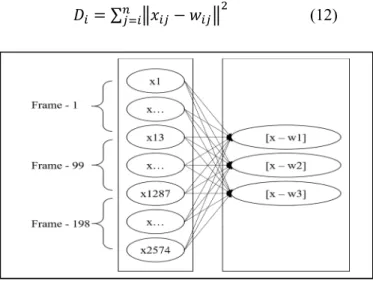
Learning Vector Quantization (LVQ) is a supervised version of vector quantization that can be used when we have each input data with class label. This learning technique uses the class information to reposition the Voronoi vectors slightly to improve the quality of the classifier decision regions, which adapted from Kohenen Map. It is a two stage process of LVQ as shown Fig. 3. Input of LVQ is Ceptrum result that 198 point or number of n.
The first step is feature selection – the unsupervised identification of a reasonably small set of features in which the essential information content of the input data is concentrated. The second step is the classification where the feature domains are assigned to individual classes.
The basic LVQ algorithm is simple. It starts to set representative data each i class that called as weight wi. Each set supervised training data, found distance each i class:
-400 -200 0 200 400 600 800 1 11 21 31 41 51 61 71 81 91 101 111 121 131 141 151
= ∑
−
(12)
Fig. 3. LVQ Architecture
The LVQ algorithm attempts to correct winning weight wi which minimum D. The correction by shifting the boundaries: 1. If the input xi and wining wi have same class label, then
move them closer together by ∆ ( ) = ( )( − ) 2. If the input xi and wining wi have different class label, then
move them apart together by ∆ ( ) = − ( )( − ) 3. Voronoi vectors/weights wj corresponding to other input
regions are left unchanged with ∆wi (t) = 0.
Where β(t) is a learning rate that decreases with the number of epochs of training. In this way we get better classification than by the SOM alone.
III. RESULT AND DISCUSSION
This research used 180 data training obtained from six subjects which 3 men and 3 women, variation of old, young and children. Each subject spoken word (“Klasik”, “Dangdut”, and “Pop” in Indonesian language). Each subject recorded 10 trials. We used two ways, first used SNR <10db and second used SNR> 60dB.
The voice signals is recorded through the microphone for ± 2 seconds and processed with Silence Removal to equalize the sound signal duration. Further data is extracted using MFCC to obtain the Cepstrum coefficient containing information from the sound signal. The extraction results as in Fig. 4.
Fig. 4. Extraction process using MFCC
The coefficient of Cepstrum used is 13 coefficients in each frame, so the result of MFCC that is coefficient of Cepstrum is 2574 coefficients.
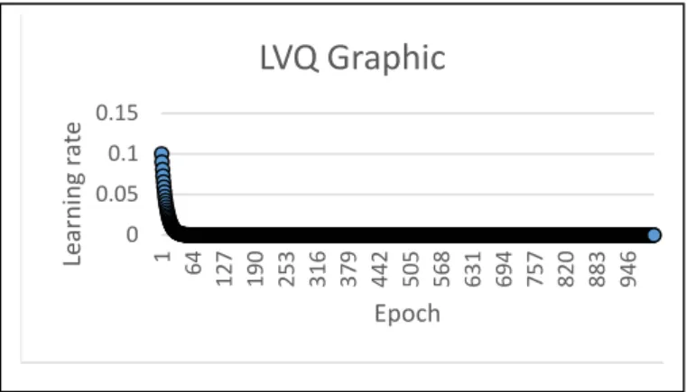
Optimized training parameters of LVQ are α 0.01 to 0.03 with 0.01 of learning rate reduction, as well as α using 0.10 to 0.10 learning rate reduction, the maximum epoch of 1000, and the minimum learning rate 0.0001. Analysis of LVQ learning rate training can be seen in Table I.
TABLE I. OPTIMIZED OF TRAINING PARAMETER No α Decrease α Training Data Accuracy (%) New Data
1 0.01 0.01 90 61.5
2 0.03 0.01 90 62.0
3 0.05 0.01 88 65.0
4 0.10 0.10 92 75.5
The results of the analysis in Table I shows that the highest accuracy is obtained with α 0.1 and decreased learning rate 0.1, so that LVQ training parameters used are α 0.1, the maximum epoch 1000, the minimum learning rate is 0.0001, and the reduction of α 0.1. The test results of 180 training data is shown in Table II.
Testing results obtained of 92% accuracy for data that has been trained and 46% for new data. However, based on the results of the evaluation of the previous test, then re-recording new data using the same SNR with the train data (SNR> 60dB). Accuracy of new test data increased to 75.5% compared to using different SNR (SNR <10dB) 46%.
In addition, the use of pre-processing greatly affects the accuracy of system testing. Training using pre-processing yields 6% higher accuracy than training without pre-processing. While training without Histogram Equalization yields 5% better accuracy than training using Histogram Equalization, this is because the acquisition data has a size close to the specified target of 16000 for each recording, as represented in Table II.
TABLE II. SYSTEM TESTING EACH 10 TIMES No Subject Class Training Data Number of recognized New Data
1 1 Klasik 10 9 2 1 Dangdut 10 9 3 1 Pop 10 7 4 2 Klasik 7 9 5 2 Dangdut 10 8 6 2 Pop 10 5 7 3 Klasik 9 8 8 3 Dangdut 10 7 9 3 Pop 7 6 10 4 Klasik 9 9 11 4 Dangdut 10 8 12 4 Pop 9 7 13 5 Klasik 10 9 14 5 Dangdut 10 7 15 5 Pop 7 8 16 6 Klasik 9 9 17 6 Dangdut 10 6 18 6 Pop 8 5 Total Recognized 165 136 Windowing Filterbank
The training process will stop when the learning rate has reached the minimum limit or reached the maximum epoch that has been determined. The computational threshold limit is determined by the epoch maximum and the learning rate set. The change of learning rate for each iteration can be seen in Fig. 5.
Fig. 5. Decrease of learning rate in training
The effect of pre-processing on the accuracy of system testing can be seen in Tabel III.
TABLE III. USING MFCC TOWARD ACCURACY
α Minimum Learning Rate
Accuracy (%)
With MFCC Without MFCC
Training
Data Data New Training Data New Data
0.1 0.0010 91 71,0 87 62
0.1 0.0001 92 75.5 86 62
Table III shows that identification using pre-processing have almost had the same accuracy compared to without pre-processing.
Accuracy results obtained from system testing are influenced by the combination of training parameters and the weight of the representatives of each randomly selected class. In addition, the use of different SNRs during recording affects the accuracy of the system towards the introduction of new data. The use of the same SNR can obtain higher test accuracy. To facilitate the use of the system, the computational model has been implemented in the form of software.
IV. CONCLUSION
This research has developed spoken word identification using Mel-Frequency Cepstrum Coefficients and Learning Vector Quantization after passed pre-processing with Histogram Equalization, DC Removal and Pre-emphasize. Optimization of LVQ parameter got 1000 maximum epoch, 0.0001 minimum of learning rate, α=0.1.
The accuracy of the testing results is 92% for identification of training set while testing new data recorded using different SNR obtained an accuracy of 46%. However, the test results of new data recorded using the same SNR with training data have got the accuracy of 75.5%.
REFERENCES
[1] S. R. Shahamiri and S. S. Binti Salim, “Artificial neural networks as speech recognisers for dysarthric speech: Identifying the
best-performing set of MFCC parameters and studying a speaker-independent approach,” Adv. Eng. Informatics, vol. 28, no. 1, pp. 102–110, 2014. [2] C. Aruna, A. D. Parameswari, M. Malini, and G. Gopu, “Voice
recognition and touch screen control based wheel chair for paraplegic persons,” in Proceeding of the IEEE International Conference on Green Computing, Communication and Electrical Engineering, ICGCCEE 2014, 2014, pp. 1–5.
[3] I.-J. Ding and S.-K. Lin, “Performance Improvement of Kinect Software Development Kit–Constructed Speech Recognition Using a Client– Server Sensor Fusion Strategy for Smart Human–Computer Interface Control Applications,” IEEE Access, vol. 5, pp. 1–1, 2017.
[4] S. R. Jaybhaye and B. Pune, “Dynamic Speech Recognition System To Control Home Appliances,” no. 5, pp. 27–32, 2015.
[5] M. Sadek Ali, “Gender Recognition System Using Speech Signal,” Int. J. Comput. Sci. Eng. Inf. Technol., vol. 2, no. 1, pp. 1–9, 2012. [6] A. Zabidi, W. Mansor, L. Y. Khuan, R. Sahak, and F. Y. A. Rahman,
“Mel-frequency cepstrum coefficient analysis of infant cry with hypothyroidism,” in Proceedings of 2009 5th International Colloquium on Signal Processing and Its Applications, CSPA 2009, 2009, pp. 204– 208.
[7] N. J. Nalini and S. Palanivel, “Music emotion recognition: The combined evidence of MFCC and residual phase,” Egypt. Informatics J., vol. 17, no. 1, pp. 1–10, 2016.
[8] M. Sahidullah and G. Saha, “Design, analysis and experimental evaluation of block based transformation in MFCC computation for speaker recognition,” Speech Commun., vol. 54, no. 4, pp. 543–565, 2012.
[9] J. Nirmal, M. Zaveri, S. Patnaik, and P. Kachare, “Novel approach of MFCC based alignment and WD-residual modification for voice conversion using RBF,” Neurocomputing, vol. 237, no. September, pp. 39–49, 2017.
[10] J. Nirmal et al., “Artificial neural networks as speech recognisers for dysarthric speech: Identifying the best-performing set of MFCC parameters and studying a speaker-independent approach,” Adv. Eng. Informatics, vol. 28, no. 1, pp. 102–110, 2017.
[11] V. Tiwari, “MFCC and its Applications in Speaker Recognition,” International Journal on Emerging Technologies,” Int. J. Emerg. Technol., vol. 1, no. 1, pp. 19–22, 2010.
[12] U. Bhattacharjee et al., “A Comparative Study Of LPCC And MFCC Features For The Recognition Of Assamese Phonemes,” Int. J. Eng. Res. Technol., vol. 2, no. 1, pp. 2–6, 2013.
[13] Ranny, “Voice Recognition using k Nearest Neighbor and Double Distance Method,” in 2016 International Conference on Industrial Engineering, Management Science and Application (ICIMSA), 2016, pp. 1–5.
[14] M. Abe, S. Nakamura, K. Shikano, and H. Kuwabara, “Voice conversion through vector quantization,” ICASSP-88., Int. Conf. Acoust. Speech, Signal Process., vol. 2, pp. 655–658, 1988.
[15] V. Dyck and F. Wuyts, “Wavelet-FILVQ for Speech Analysis,” in 13th International Conference on Pattern Recognition, 1996, no. 1, p. 214 218.
[16] E. Mansour, M. S. Sayed, A. M. Moselhy, and A. A. Abdelnaiem, “LPC and MFCC Performance Evaluation with Artificial Neural Network for Spoken Language Identification,” Int. J. Signal Process. Image Process. Pattern Recognit., vol. 6, no. 3, pp. 55–66, 2013.
[17] S. Farah and A. Shamim, “Speaker recognition system using mel-frequency cepstrum coefficients, linear prediction coding and vector quantization,” in 2013 3rd IEEE International Conference on Computer, Control and Communication, IC4 2013, 2013.
[18] A. H. Mansour, K. A. Mohammed, and G. Z. Alabdeen Salh, “Voice Recognition using Dynamic Time Warping and Mel-Frequency Cepstral Coefficients Algorithms,” Int. J. Comput. Appl., vol. 116, no. 2, pp. 34– 41, 2015.
[19] U. Bhattacharjee, “A comparative study of LPCC and MFCC features for the recognition of Assamese phonemes,” Int. J. Eng. Res. Technol., vol. 2, no. 3, pp. 1–6, 2013.
[20] J. Mantysalo, K. Torkkola, T. K. Kohonen, and C. Science, “LVQ-based Speech Recognition with High-Dimensional Context Vectors Abstract 2 Speech data and preprocessing 1 Introduction 3 LVQ-based separate phoneme recognition,” October, vol. 1, pp. 539–542, 1992.
[21] K. M. O. Nahar, M. A. Shquier, W. G. Al-Khatib, H. Al-Muhtaseb, and M. Elshafei, “Arabic phonemes recognition using hybrid LVQ/HMM
0 0.05 0.1 0.15 1 64 127 190 253 316 379 442 505 568 631 694 757 820 883 946 Le arni ng rate Epoch
LVQ Graphic
model for continuous speech recognition,” Int. J. Speech Technol., vol. 19, no. 3, pp. 495–508, 2016.
[22] M. Gales and S. Young, “The Application of Hidden Markov Models in Speech Recognition,” Found. Trends® Signal Process., vol. 1, no. 3, pp. 195–304, 2007.
[23] V. Tiwari, “MFCC and its applications in speaker recognition,” Int. J. Emerg. Technol., vol. 1, no. 1, pp. 19–22, 2010.
[24] A. Maesa, F. Garzia, M. Scarpiniti, and R. Cusani, “Text Independent Automatic Speaker Recognition System Using Mel-Frequency Cepstrum Coefficient and Gaussian Mixture Models,” J. Inf. Secur., vol. 3, no. 4, pp. 335–340, 2012.
[25] R. A. Metzger, J. F. Doherty, and D. M. Jenkins, “Analysis of compressed speech signals in an Automatic Speaker Recognition system,” 2015 49th Annu. Conf. Inf. Sci. Syst. CISS 2015, 2015.
[26] E. C. Djamal, M. Y. Abdullah, and F. Renaldi, “Brain Computer Interface Game Controlling Using Fast Fourier Transform and Learning Vector Quantization,” J. Telecommun. Electron. Comput. Eng., 2017. [27] S. M. S. Manasa C, Thejaswini S, “Brain Computer Interface Systems
To Assist Patients Using EEG Signals,” Int. J. Innov. Res. Comput. Commun. Eng., vol. 3, no. 6, pp. 4994–5001, 2015.
[28] P. Bisnis, I. Dengan, and T. Olap, “Prosiding SNST ke-7 Tahun 2016 Fakultas Teknik Universitas Wahid Hasyim Semarang 7,” pp. 7–12, 2016.
[29] T. D. Ganchev, “Speaker Recognition,” University of Patras, Greece, 2005.