Constraints Preserving Genetic Algorithm for
Learning Fuzzy Measures with an Application to
Ontology Matching
Mohammad Al Boni1, Derek T. Anderson2, and Roger L. King3 1,3
Center for Advanced Vehicular Systems Mississippi State University, MS 39762 USA
1
[email protected],[email protected] 2Electrical and Computer Engineering Department
Mississippi State University, MS 39762 USA
Abstract. Both the fuzzy measure and integral have been widely stud-ied for multi-source information fusion. A number of researchers have proposed optimization techniques to learn a fuzzy measure from train-ing data. In part, this task is difficult as the fuzzy measure can have a large number of free parameters (2N−2 for N sources) and it has
many (monotonicity) constraints. In this paper, a new genetic algorithm approach to constraint preserving optimization of the fuzzy measure is present for the task of learning and fusing different ontology matching results. Preliminary results are presented to show the stability of the leaning algorithm and its effectiveness compared to existing approaches.
Keywords: Fuzzy measure, fuzzy integral, genetic algorithm, ontology matching
1
Introduction
The fuzzy integral (FI), introduced by Sugeno [14], is a powerful tool for data fusion and aggregation. The FI is defined with respect to a fuzzy measure (FM). The FM encodes the worth of different subsets of sources. Successful uses of the FI include, to name a few, multi-criteria decision making [6], image processing [15], or even in robotics [12].
It is well-known that different FMs lead the FI, specially the Choquet FI, to behave like various operators (max, min, mean, etc.) [15]. In some applica-tions, we can define the FM manually. However, in other settings, it may only be possible to define the densities (the measures on just the singletons) and a measure building technique is used e.g., a S-Decomposable measure such as the Sugeno λ-fuzzy measure. It is also very difficult, if possible at all, to specify a FM for relatively smallN (number of inputs), as the lattice already has 2N −2
free parameters! (e.g., forN = 10 inputs, 210−2 = 1022 free parameters). Also, input sources can be of different nature. For example, we may fuse values from
sensors with algorithms outcomes. In such problems, it is hard to determine the importance of each input data source. Thus, many data-driven learning methods are used to learn the measure. One method is to use a quadratic program (QP) to learn the measure based on a given data set [6]. Although the QP is an effective approach to build the measure using a data set, its complexity is relatively high and it does not scale well [10]. Other optimization techniques have been used to reduce the complexity and improve performance, e.g., genetic algorithms (GA) [2]. The goal of this article is to design and implement a GA to learn the full FM from ontology similarities. The main contribution of this article includes: the investigation of new constraint preserving operators (crossover and mutation) in a GA that overcome drawbacks of prior work. The application of this theory is to learn a FM to fuse multiple similarity techniques in the context of ontology matching.
2
Related Work in Ontologies
A number of works have been put forth in the literature regarding combining several ontology matching techniques. In [18], Wang et al. used Dempster Shafer theory (DST) to combine results obtained from different ontology matcher. Each result is treated as a mass function and combined using the Dempster’s Com-bination Rule. It is not clear that DST is the correct fit because in DST one typically only has access to a limited amount of evidence in different focal sets. However, the authors appear to have access to all information in the form of on-tology term matching matrices. Other papers, such as [9, 17], have used a GA to learn the weight of each matching algorithm for an operator like a weighted sum. Herein, an improved set of constraint preserving GA operators are put forth and more powerful non-linear aggregation operator, the FI, is investigated.
3
Fuzzy Integral and Fuzzy Measure
For a set ofN input sources,X ={x1, x2, ..., xN}, the discrete FI is: Z s h◦g= N _ i=1 h(xπ(i))∧G(xπ(i)) , (1)
where his the partial support function,h:X →[0,1],h(xπ(i)) is the evidence
provided by source π(i), π is a re-permutation function such that h(xπ(1)) ≥ h(xπ(2)) ≥ ... ≥ h(xπ(N)). The value G(xπ(i)) = g({xπ(1), xπ(2), ..., xπ(i)}) is
the measure of a set of information sources. Note,R
sh◦g is bounded between N V i=1 h(xi), N W i=1 h(xi)
and it can be explained in words as “the best pessimistic agreement”.
The FM can be discussed in terms of its underlying lattice. A lattice is induced by the monotonicity constraints over the set 2N. Each node or vertex
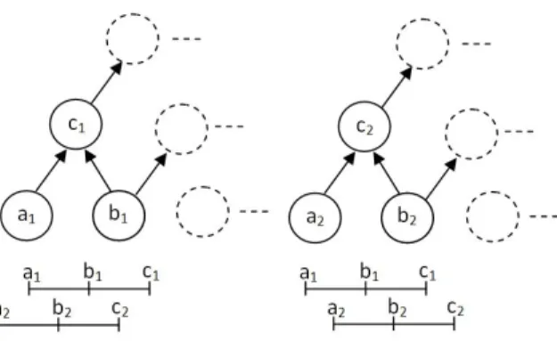
in the lattice is the measure for a particular subset of sources, e.g.,g({x1, x3}). Figure 1a is an illustration of the FM for N = 3. Formally, a FM, g, is a set-valued function g : 2X → [0,1], whereg(∅) = 0,g(X) = 1, and for A, B ⊆X,
such thatA⊆B, g(A)≤g(B) (the monotonicity constraint).
(a) Lattice view of a FM.
(b) Interval view of a monotonicity con-straint.
Fig. 1: (a) FM lattice for N = 3 and (b) possible values for g({x1, x3}) for a giveng({x1}) andg({x3}).
4
Preserving FM Constraints in a Genetic Algorithm
Many previous attempts exist to address constraint satisfaction in a GA. Typ-ically, a penalty function is used to reduce the fitness of solutions that violate constraints [11]. However, even if infeasible solutions are close to an ideal mini-mum, it is not clear why or how to really balance the cost function to eventually help it converge to a quality valid solution. In the FM, we have an exponentially increasing number of constraints in N. It is a highly constrained problem. It is not likely that we will end up obtaining a valid FM for such a heavy constrained problem (or that one such infeasible solution could simply be made a quality feasible solution at the end). Therefore, penalty function strategy becomes very risky to use and will restrain the search space. Many researchers avoid dealing with the FM constraints by designing a GA that learn only the densities. Then, the rest of the lattice is populated using a measure deriving technique such as the Sugenoλ-fuzzy measure. However, a better solution is to design a more intel-ligent set of GA operators for the constraints in a FM so we can efficiently search just the valid FM space and operate on valid FMs. Since all chromosomes in a population are always valid (started and remained valid by using our crossover and mutation operators), we did not have to modify the selection process. Only crossover and mutation need be defined to preserve the monotonicity constraints.
4.1 Constraint preserving crossover for the FM
In this subsection, a new GA crossover operation is described that preserves the monotonicity property of the FM. First, g(∅) and g(X) need not be considered as they are 0 and 1 by definition. It is the remaining 2N −2 lattice elements that we are concerned with. In order to ensure a valid FM after crossover, we decompose the FM into a set of interval relations that present the allowable bounds for crossover. For example, consider a set {x1, x3} of sources,{x1} and {x3}, such that g({x1}) =a, g({x3}) = b and g({x1, x3}) = c. We know from the FM thatmax(a, b)≤c. Figure 1b illustrates the valid interval ranges that
a,b andccan posses in order to remain a valid (credible) FM.
Definition 1 (Intersected and non-inclusive intervals).Letd= [d1, d2], e= [e1, e2] be two intervals such thatd∩e6=∅. Letdbe the smaller of the two inter-vals, i.e.,d2−d1< e2−e1. Ifd1≤e1 ord2≥e2then we calldandeintersected and non-inclusive intervals.
Note, this property is needed herein in order to identify candidate chromo-somes to perform crossover on.
Definition 2 (Random density crossover).Letg1andg2 be two FMs. Let ↔denote the random selection and swapping of one density fromg1,b1=g1(xi),
andg2,b2=g2(xj), wherei,j are random numbers in{1,2, .., N}.
Note, by itself,↔does not guarantee a valid FM.
Definition 3 (Repair operator for ↔). Let ⇔ (explained in Prop 1) de-note an operation to repair a violation of the monotonicity constraint caused by ↔.
Even though we discuss crossover of densities (↔), ⇔has the result that it impacts multiple layers in the FM. As such, while we only cross two densities, we are in fact changing many values in a FM. It is important to note that our ⇔makes use of existing values in the FM to repair any violations in the other FM. This means no “new” information is injected, rather the values in two FMs are swapped (in the classical theme of crossover).
Proposition 1:Letg1andg2be two FMs withNinput sources and let the mea-sure on the densities{{x1},{x2}, ...,{xN}}be{g11, g12, ..., g1N}and{g21, g22, ..., gN2} respectively. Furthermore, let each measure be sorted individually such that
gπ1(1) 1 ≤g π1(2) 1 ≤...≤g π1(N) 1 and g π2(1) 2 ≤g π2(2) 2 ≤...≤g π2(N) 2 whereπ1,π2 are re-permutation functions. Furthermore, we make the assumption that each cor-responding sorted sub-interval is intersected and non-inclusive between g1 and
g2 (Def.1). Then, all admissible ↔ (Def.2), followed by ⇔ (Def.3), operations are guaranteed to not violate the FM monotonicity property.
Proof: This proposition is proved by considering all possible enumerable cases. First, we divide the problem into identical sub-problems, and we prove the propo-sition for the case of one interval pair. Next, this single case is extended to the
Fig. 2: Two FMs with possible range conditions for swapping values across mea-sures.
case of multiple corresponding interval pairs.
First,g1 and g2 are individually sorted. Then, the intervals [g
π1(1) 1 , g π1(N) 1 ] and [gπ2(1) 2 , g π2(N)
2 ] are divide into sub-intervals, each with two sources i.e.,{[g
π1(1) 1 , gπ1(2) 1 ],[g π1(2) 1 , g π1(3) 1 ], ..., [g π1(N−1) 1 , g π1(N) 1 ]} and {[g π1(1) 2 , g π1(2) 2 ],[g π1(2) 2 , g π1(3) 2 ], ..., [gπ1(N−1) 2 , g π1(N)
2 ]}. Next, we look at the case of a single corresponding interval pair betweeng1andg2. Leta1=g
π1(1) 1 ,b1=g π1(2) 1 ,a2=g π2(1) 2 andb2=g π2(2) 2 .
Since [a1, b1],[a2, b2] are intersected and non-inclusive intervals (Def.1), then we have two cases (see Figure 2):
a2≤a1≤b2≤b1 (2)
a1≤a2≤b1≤b2 (3)
For case 2, there are four admissible crossover operations:
(1)a1↔a2: no need to swapc1 andc2and the new intervals are [a2, b1],[b1, c1] and [a1, b2],[b2, c2].
(2)a1↔b2: Sinceb2≤b1, the new intervals are [b2, b1],[b1, c1] and [a2, a1],[a1, c2]. No need to swapc1 andc2.
(3)b1↔a2: Swapc1⇔c2. The new intervals are [a2, a1],[a1, c2] and [b2, b1],[b1, c1]. (4)b1↔b2: Swapc1⇔c2. The new intervals are [a1, b2],[b2, c2] and [a2, b1],[b1, c1]. Case 3 is proved the same way i.e., perform↔then check the resulted intervals and apply ⇔when required. Because↔is applied on one density in each FM, the proof of the first sub-interval case is easily generalized to the other cases. Since Def.1 holds, we randomly select one density in g1 to be swapped with a different randomly swapped density ing2. Then,⇔is iteratively repeated up the lattice to fix all violations resulting from the↔ operator. At each layer in the lattice, which means for all measure values on sets of equal cardinality, intervals are compared and⇔is applied when required.
4.2 Constraints preserving mutation
In mutation, a random value in the lattice will be changed. In order not to violate the monotonicity constraint, the new value of a randomly selected node, should be greater than or equal the maximum measure of the nodes coming into it and less than or equal the minimum measure of those it goes into at the next layer. This is the only required modification to the traditional mutation by restricting the new value between a minimum and maximum thresholds.
5
Application: Ontology matching with the fuzzy integral
Ontologies are used in different knowledge engineering fields, for example the semantic web. Because it is widely used, many redundant ontologies have been created and many ontologies may fully, or partially, overlap. Matching these redundant and heterogeneous ontologies is an on-going research topic. A good survey is presented in [1]. However, the no-free-lunch theorem was proven, i.e., no algorithm can give the optimal ontology matching among all knowledge domains, due to the complexity of the problem [1]. In this section, we implement an algorithm to combine results from different similarity matching techniques using the FI. So is the claim, if we cannot outright solve it, then aggregate multiple methods to help improve the robustness of our approach.
Ontology matching is a process, applied on two ontologies, that tries to find, for each term within one ontology (the source), the best matched term in the sec-ond ontology (the destination). This problem can be approached using several mechanisms based on: string normalization, string similarity, data-type com-parison, linguistic methods, inheritance analysis, data analysis, graph-mapping, statistical analysis, and taxonomy analysis [9]. In this paper, we fused results from existing matchers: FOAM ([4]), FALCON ([7]) and SMOA ([13]).
5.1 Genetic Algorithm Implementation
Encoding: Each chromosome is a vector of [0,1]-valued numbers that map lexographically to a FM e.g., (g1, g2, ..., gN, g1,2, ..., g1,...,N−1). The length of a
chromosome is 2N −2 (where there are N similarity matching algorithms).
Fitness Function: Semantic precision and recall are widely used to evaluate the performance of ontology matching algorithms [5].They are an information retrieval metrics [16] that have been used for ontology matching evaluation since 2002 [3]. Fmeasure is a compound metric that can reflect both precision and recall, and it is given by the formula:
F measure=2∗precision∗recall
precision+recall , (4)
where precision is given by:
precision=|A∩R|
and recall is given by:
recall= |A∩R|
R , (6)
R is the reference ontology and A is the alignment resulted from the matching technique. First, the most fitted chromosome (FM) is used with the FI to calcu-late A. Then, A is used in computing precision and recall. Lastly, Fmeasure is obtained from the resulted precision and recall. The goal of our GA is to maxi-mize the Fmeasure. We linearly scaled the plot (Fig 3) to aid visual display.
Crossover: Crossover is performed in two phases. The first phase checks the intersection property between the parents’ chromosomes so they will result in a valid offspring. The second phase performs Def.2 and 3.
Selection:We adopted traditional roulette wheel selection.
Stop condition:A maximum number of iterations is used as the stopping con-dition.
5.2 Experimental Results and Evaluation
Several tests were conducted on the I3CON [8] data set. We compared the per-formance of our tool with existing tools using the precision, recall and Fmeausre (see figures 5a, 5b, 5c). Although our approach gives lower precision than FOAM, FALCON and SMOA individually, it gives a better Fmeasure. This occurs be-cause we combine several results which reduces precision but increases recall considerably. Our tool provides a precision of 1 if and only if the precision of all combined sources is 1. Also, our tool tends to give better results than GOALS. GOALS uses an OWA operator to combine results from different matchers. We conducted two experiments on the ”AnimalsA.owl” and ”AnimalsB.owl” using different OWAs. With an OW A = [0.3,0.4,0.3] (OW A = [0.7,0.2,0.1] respec-tively) we get an Fmeasure of 0.8571 (0.875 respectively) while our tool returns a value of 0.8936. Inconsiderate (underestimated or overestimated) selection of OWA values dose affect the performance of the system. Since different matchers give different results on different domains, it is difficult to choose the optimal selection of OWA that gives the best results. Our system solves this problem by using the GA to learn the weights. We can learn an OWA if its needed, or any other aggregation operators, but it does not need to be decided up front.
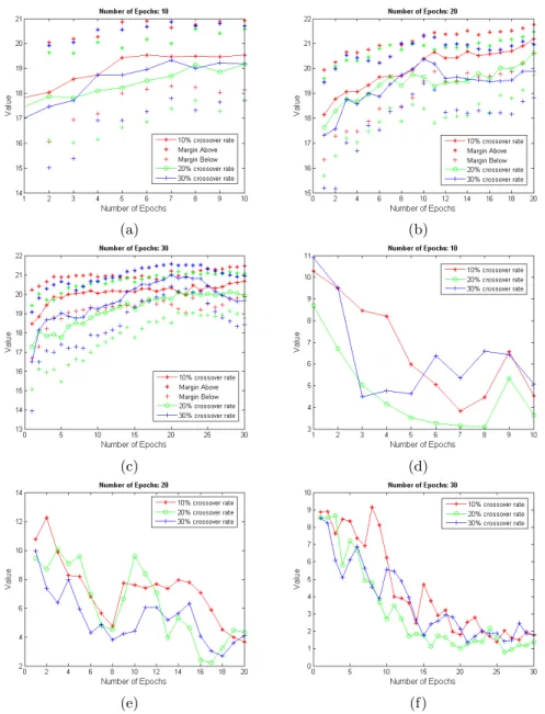
Also, figures 3a, 3b, 3c, show the convergence of the GA using 10,20, and 30 iterations with crossover rate of 0.1, 0.2 and 0.3. Each graph is the average fitness value of the population at each iteration. We also report, at each x-location, the full range bounds (max and min). By comparing the results from different configurations, we found that a 10% crossover rate with 10 iterations was enough to achieve the desired results herein. With such configurations, the GA reached convergence with minimal computational effort. Also, we found that the range bounds decreases, which reflects convergence over time. Moreover, we found that all of the plots decrease at some point. This is caused by mutation, in which we are exploring a bigger space which may not have a high fitness value. To determine the performance of the constraint preserving crossover, we conducted
two studies. Study 1 shows the average number of chromosomes that have a valid interval property (see figures 3d, 3e, 3f). This reflects the applicability of our crossover model. We notice that the average number of suitable mates tend to decrease at each iteration. That happens because chromosomes will converge more at each iteration and will likely violate the interval property. Study 2 is conducted on the average number of attempts to find a suitable mate to crossover with (see figures 4a, 4b, 4c). We found that this number tends to increase in average at each iteration because fewer chromosomes will have a valid interval property. Thus, we have less of a chance to find a valid candidate pair and the number of attempts increases.
6
Conclusion and Future Work
In this paper we propose a new constraint preserving GA for learning FMs. Specifically, we proposed a new crossover and mutation operation and different ontology matching algorithms were fused using the FI learned by the GA. We showed that our framework can give satisfactory results on different study do-mains. However, a few challenges need to be extended for future work, e.g., we would like to explore the use of the shapely index to determine the importance of each matching algorithm. Also, we will study the use of more than two ontologies to support the matching between ontologies. Also, the decreasing trend of the average number of matches raises an important question. What if we had to run the algorithm for a long time, would we reach a starvation (a case in which we can’t find a valid candidate to crossover with)? If yes, do we need to relax our constraints? If we could not, could we design a new operator that can insert new valid candidates to keep the algorithm moving? Passing multiple populations? Point being, need to revisit the harsh constraints on learning. Likewise, we would like to explore the use of island GAs on different populations which may help increase the chance of success and diversity.
7
Acknowledgments
The first author would like to acknowledge and thank the Fulbright scholarship program for its financial support of the work performed herein.
References
1. S. Amrouch and S. Mostefai. Survey on the literature of ontology mapping, align-ment and merging. InInformation Technology and e-Services (ICITeS), 2012 In-ternational Conference on, pages 1–5. IEEE, 2012.
2. D. T. Anderson, J. M. Keller, and T. C. Havens. Learning fuzzy-valued fuzzy measures for the fuzzy-valued sugeno fuzzy integral. InComputational Intelligence for Knowledge-Based Systems Design, pages 502–511. Springer, 2010.
3. H.-H. Do, S. Melnik, and E. Rahm. Comparison of schema matching evaluations. InProc. Workshop on Web, Web-Services, and Database Systems, volume 2593 of
Lecture notes in computer science, pages 221–237, Erfurt (DE), 2002.
4. M. Ehrig and Y. Sure. Foam-framework for ontology alignment and mapping-results of the ontology alignment evaluation initiative. InWorkshop on integrating ontologies, volume 156, pages 72–76, 2005.
5. J. Euzenat. Semantic precision and recall for ontology alignment evaluation. In
Proc. 20th International Joint Conference on Artificial Intelligence (IJCAI), pages 348–353, 2007.
6. M. Grabisch. The application of fuzzy integrals in multicriteria decision making.
European journal of operational research, 89(3):445–456, 1996.
7. W. Hu and Y. Qu. Falcon-ao: A practical ontology matching system.Web Seman-tics: Science, Services and Agents on the World Wide Web, 6(3):237–239, 2008. 8. I. Interpretation and I. Conference. Ontology Alignment Dataset. http://www.
atl.lmco.com/projects/ontology/i3con.html, 2004. [accessed 4-June-2013]. 9. J. Martinez-Gil, E. Alba, and J. F. Aldana-Montes. Optimizing ontology
align-ments by using genetic algorithms. InProceedings of the workshop on nature based reasoning for the semantic Web. Karlsruhe, Germany, 2008.
10. A. Mendez-Vazquez and P. Gader. Sparsity promotion models for the choquet integral. In Foundations of Computational Intelligence, 2007. FOCI 2007. IEEE Symposium on, pages 454–459. IEEE, 2007.
11. Z. Michalewicz. Genetic algorithms, numerical optimization, and constraints. In
Proceedings of the Sixth International Conference on Genetic Algorithms, volume 195, pages 151–158. Morgan Kaufmann, San Mateo, CA, 1995.
12. G.-Y. Pan, W.-Y. Wang, C.-P. Tsai, W.-Y. Wang, and C.-R. Tsai. Fuzzy measure based mobile robot controller for autonomous movement control. InSystem Science and Engineering (ICSSE), 2011 International Conference on, pages 649–653, 2011. 13. G. Stoilos, G. Stamou, and S. Kollias. A string metric for ontology alignment. In
The Semantic Web–ISWC 2005, pages 624–637. Springer, 2005.
14. M. Sugeno. Theory of fuzzy integrals and its applications. PhD thesis, Tokyo Institute of Technology, 1974.
15. H. Tahani and J. M. Keller. Information fusion in computer vision using the fuzzy integral. Systems, Man and Cybernetics, IEEE Trans on, 20(3):733–741, 1990. 16. C. J. K. van Rijsbergen.Information retrieval. Butterworths, London (UK), 1975.
http://www.dcs.gla.ac.uk/Keith/Preface.html.
17. J. Wang, Z. Ding, and C. Jiang. Gaom: genetic algorithm based ontology matching. InServices Computing, 2006, pages 617–620. IEEE, 2006.
18. Y. Wang, W. Liu, and D. Bell. Combining uncertain outputs from multiple ontol-ogy matchers. InScalable Uncertainty Mgmt., pages 201–214. Springer, 2007.
(a) (b)
(c) (d)
(e) (f)
Fig. 3: (a)(b)(c) Analysis of GA behavior and performance for different num-ber of epochs (10,20,30) and different crossover rates (10%,20%,30%.) (d)(e)(f) Average number of chromosomes with a valid interval property.
(a) (b)
(c)
Fig. 4: (a)(b)(c) Average number of attempts to find a chromosome with a valid interval property.
(a) (b) (c)
Fig. 5: (a)(b)(c) Ontology matching evaluation metrics: precision, recall, Fmea-sure.
![Figure 1a is an illustration of the FM for N = 3. Formally, a FM, g, is a set- set-valued function g : 2 X → [0, 1], where g(∅) = 0, g(X) = 1, and for A, B ⊆ X, such that A ⊆ B, g(A) ≤ g(B) (the monotonicity constraint).](https://thumb-us.123doks.com/thumbv2/123dok_us/859047.2609533/3.918.224.707.291.486/figure-illustration-fm-formally-valued-function-monotonicity-constraint.webp)