Delay-Based Back-Pressure Scheduling in
Multi-Hop Wireless Networks
Bo Ji
Department of ECE The Ohio State UniversityEmail: [email protected]
Changhee Joo
Department of EECEKorea University of Technology and Education, Korea
Email: [email protected]
Ness B. Shroff
Departments of ECE and CSEThe Ohio State University Email: [email protected]
Abstract—Scheduling is a critical and challenging resource allocation mechanism for multi-hop wireless networks. It is well known that scheduling schemes that give a higher priority to the link with larger queue length can achieve high throughput performance. However, this queue-length-based approach could potentially suffer from large (even infinite) packet delays due to the well-known last packet problem, whereby packets may get excessively delayed due to lack of subsequent packet arrivals. Delay-based schemes have the potential to resolve this last packet problem by scheduling the link based on the delay for the packet has encountered. However, the throughput performance of delay-based schemes has largely been an open problem except in limited cases of single-hop networks. In this paper, we investigate delay-based scheduling schemes for multi-hop traffic scenarios. We view packet delays from a different perspective, and develop a scheduling scheme based on a new delay metric. Through rigorous analysis, we show that the proposed scheme achieves the optimal throughput performance. Finally, we conduct extensive simulations to support our analytical results, and show that the delay-based scheduler successfully removes excessive packet delays, while it achieves the same throughput region as the queue-length-based scheme.
I. INTRODUCTION
Link scheduling is a critical resource allocation com-ponent in multi-hop wireless networks, and also perhaps the most challenging. The celebrated Queue-length-based Back-Pressure (Q-BP) scheduler [1] has been shown to be throughput-optimal and can stabilize the network under any feasible load. Since the development of Q-BP, there have been numerous extensions that have integrated it in an over-all optimal cross-layer solution. Further, easier-to-implement queue-length-based scheduling schemes have been developed and shown to be throughput-efficient (see [2] and references therein). Some recent attempts [3], [4] focus on designing real-world wireless protocols using the ideas behind these algorithms.
While these queue-length-based schedulers have been shown to achieve excellent throughput performance, they are usually evaluated under the assumption that flows have an infinite amount of data and keep injecting packets into the network. However, in practice accounting for multiple time scales [5]–[7], there also exist other types of flows that have
This work was supported in part by NSF award CNS-0721236 and ARO MURI project W911NF-08-1-0238.
a finite number of packets to transmit, which can result in the well-known last packet problem: consider a queue that holds the last packet of a flow, then the packet does not see any subsequent packet arrivals, and thus the queue length remains very small and the link may be starved for a long time, since the queue-length-based schemes give a higher priority to links with a larger queue length. In such a scenario, it has also been shown in [5] that the queue-length-based schemes may not even be throughput-optimal.
Recent works in [8]–[13] have studied the performance of delay-based scheduling algorithms that use the Head-of-Line (HOL) delay instead of queue length as link weight. One desirable property of the delay-based approach is that they provide an intuitive way around the last packet problem. The schedulers give a higher priority to the links with a larger weight as before, but the weight (i.e., the HOL delay) of a link increases with time until the link gets scheduled. Hence, if the link with the last packet is not scheduled at this moment, it is more likely to be scheduled in the next time. However, the throughput performance of the delay-based scheduling schemes is not fully understood, and has merely been shown for limited cases of single-hop networks.
The delay-based approach was introduced in [8] for schedul-ing in Input-Queued switches. The results have been ex-tended to wireless networks for single-hop traffic, providing throughput-optimal delay-based MaxWeight scheduling algo-rithms [10], [11], [14]. It is also shown that delay-based schemes with appropriately chosen weight parameters also provide good Quality of Service (QoS) [9], and can be used as an important component in a cross-layer protocol design [13]. The performance of the delay-based MaxWeight scheduler has been further investigated in a single-hop network with flow dynamics [12]. The results show that, when flows arrive at the base station carrying a finite amount of data, the delay-based MaxWeight scheduler achieves the optimal throughput performance while its queue-length-based counterpart does not.
However, in multi-hop wireless networks, the throughput performance of these delay-based schemes has largely been an open problem. To the best of our knowledge, there are no prior works that employ delay-based algorithms to address the important issue of throughput-optimal scheduling in wireless
networks with multi-hop traffic. The problem turns out to be far more challenging in the multi-hop scenario due to the following reason. In [11], the key idea in showing throughput optimality of the delay-based MaxWeight scheduler is to exploit the following property: after a finite time, there exists a linear relation between queue lengths and HOL delays, where the ratio is the mean arrival rate. Hence, the delay-based MaxWeight scheme is basically equivalent to its queue-length-based counterpart, and thus achieves the optimal throughput. This property holds for the single-hop traffic, since given that the exogenous arrival processes follow the Strong Law of Large Numbers (SLLN) and the fluid limits exist, the arrival processes turn out to be deterministic processes with constant rates in the fluid limits. However, such a linear relation does not necessarily hold for the multi-hop traffic, since the packet arrival rate at a non-source node (or a relay node) is not a constant and depends on the underlying scheduler’s dynamics. To this end, we investigate delay-based scheduling schemes that achieve the optimal throughput performance in multi-hop wireless networks.
Unlike previous delay-based schemes, we view packet delay as a sojourn time in the network, and re-design the delay metric of a queue as the delay difference between the queue’s HOL packet and the HOL packet of its previous hop (see Eq. (34) for the formal definition). Using this new metric, we can establish a linear relation between queue lengths and delays in the fluid limit model. Then the linear relation plays the key role in showing that the proposed Delay-based Back-Pressure (D-BP) scheduling scheme is throughput-optimal in multi-hop networks.
In summary, the main contributions of our paper are as follows:
• We re-visit throughput optimality of Q-BP using fluid limit techniques. Throughput optimality of Q-BP has been originally shown using the standard Lyapunov tech-nique in a stochastic sense. We re-derive throughput optimality of Q-BP itself using fluid limit techniques so that we can extend the analysis to D-BP using the linear relation between queue lengths and delays in the fluid limit model.
• We devise a new delay metric for D-BP and show that it achieves the optimal throughput performance in multi-hop wireless networks. Calculating a link weight as sojourn time difference of the HOL packet, we establish a linear relation between queue lengths and delays in the fluid limit model, which leads to throughput-optimality of D-BP following the same analytical procedure of Q-BP. • We conduct extensive simulations to evaluate the
perfor-mance of delay-based schedulers. Through simulations, we observe that the last packet problem can cause ex-cessive delays for certain flows under Q-BP, while the problem is eliminated under D-BP. Further, in the case of Q-BP, even though the average delays experienced in the network may be similar to D-BP, the tail of the delay distribution could be substantially longer. We also show that, D-BP can not only achieve the same throughput
region as Q-BP, but also guarantee better fairness by scheduling the links based on delays and not starving certain flows that lack subsequent packet arrivals (or have very large inter-arrival times between groups of packet arrivals).
The remainder of the paper is organized as follows. In Section II, we present a detailed description of our system model. In Section III, we show throughput optimality of Q-BP using fluid limit techniques, and extend the analysis to D-BP in Section IV. We evaluate the performance of delay-based schedulers through simulations in Section V, and conclude our paper in Section VI.
II. SYSTEMMODEL
We consider a multi-hop wireless network described by a directed graph G = (V,E), where V denotes the set of nodes and E denotes the set of links. Nodes are wireless transmitters/receivers and links are wireless channels between two nodes if they can directly communicate with each other. We assume a time-slotted system with a single frequency channel. During a single time slot, multiple links that do not interfere can be active at the same time, and each active link transmits one packet during the time slot if its queue is not empty. Let S denote the set of flows in the network. We assume that each flow has a single, fixed, and loop-free route. The route of flow s has an H(s)-hop length from the source to the destination, where each k-th hop link is denoted by (s, k). Note that the assumption of single route and unit capacity is for ease of exposition, and one can easily extend the results to more general networks with multiple fixed routes and heterogeneous capacities. To specify wireless interference, we consider thek-th hop of each flowsor link-flow-pair (s, k). Let P denote the set of all link-flow-pairs, i.e., P ,{(s, k) | s∈ S, 1 ≤k≤H(s)}. The set of link-flow-pairs that interfere with (s, k)can be described as
I(s, k),{(r, j)∈ P |(s, k)interferes with(r, j),
or(r, j) = (s, k)}. (1)
Note that the interference model we adopt is general. A schedule is a set of (active or inactive) link-flow-pairs, and can be represented by a vector M~ ∈ {0,1}|P|, where each link-flow-pair is set to 1 if it is active, and 0 if it is inactive, and | · | denotes the cardinality of a set. A schedule M~ is said to be feasible if no two link-flow-pairs of M~ interfere with each other, i.e.,(r, j)∈/ I(s, k)for all(r, j),(s, k)with
Mr,j= 1andMs,k= 1. LetMP denote the set of all feasible schedules inP, and letCo(MP)denote its convex hull.
LetAs(t)denote the number of packet arrivals at the source node of flowsat time slott. We assume that the packet arrival processes satisfy the Strong Law of Large Numbers (SLLN): with probability 1,
limt→∞
Pt−1
τ=0As(τ)
t =λs, (2)
for all flow s ∈ S, and their fluid limits exist [15]. We call
λs the arrival rate of flow s, and let ~λ ,[λ1, λ2,· · ·, λ|S|] denote its vector.
Let Qs,k(t)denote the number of packets at the queue of
(s, k) at the beginning of time slot t. Slightly abusing the notation, we also useQs,kto denote the queue. We denote the
queue length vector at time slottbyQ~(t),[Qs,k(t), (s, k)∈ P], and use k · k to denote the L1-norm of a vector, e.g.,
kQ~(t)k = P
(s,k)∈PQs,k(t). Let Πs,k(t) denote the service of Qs,k at time slot t, which takes either 1 if link-flow-pair (s, k)is active, or 0, otherwise, in our settings. We denote the actual number of packets transmitted from Qs,k at time slot
t byΨs,k(t). Clearly, we have Ψs,k(t)≤Πs,k(t)for all time slots t≥0. LetPs,k(t) ,Pk
i=1Qs,i(t) denote the summed queue length of queues up to the k-th hop for flow s. By setting Qs,H(s)+1 = 0, we have Ps,H(s)+1 = Ps,H(s). The queue length evolves according to the following equations:
Qs,k(t+ 1) =Qs,k(t) + Ψs,k−1(t)−Ψs,k(t), (3) where we set Ψs,0(t) =As(t).
Let Fs(t)be the total number of packets that arrive at the source node of flow s until time slot t ≥0, including those present at time slot 0, and let Fˆs,k(t) be the total number of packets that are served at Qs,k until time slot t ≥0. We by
convention set Fˆs,k(0) = 0for all link-flow-pairs(s, k)∈ P. We letZs,k,i(t)denote the sojourn time of thei-th packet of
Qs,kin the network at time slott, where the time is measured
from when the packet arrives in the network (i.e., when the packet arrives at the source node), and letWs,k(t)denote the sojourn time of the Head-of-Line (HOL) packet of Qs,k in
the network at time slot t, i.e., Ws,k(t) = Zs,k,1(t). We set
Ws,0(t) = 0and Ws,H(s)+1(t) =Ws,H(s)(t), for all s ∈ S. Further, if Qs,k(t) = 0, we set Ws,k(t) =Ws,k−1(t). Letting
Us,k(t),t−Ws,k(t)denote the time when the HOL packet ofQs,k arrives in the network, we have that
Us,k(t) = inf{τ≤t| Fs(τ)>Fˆs,k(t)}, for all t≥0. (4) We next define the stability of a network as follows. Definition 1: A network of queues is said to be stable if,
lim supt→∞1t
Pt−1
τ=0E[kQ~(τ)k]<∞. (5) We define the throughput region of a scheduling policy as the set of rates, for which the network remains stable under this policy. Further, we define the optimal throughput region (or stability region) as the union of the throughput regions of all possible scheduling policies. The optimal throughput region
Λ∗ can be presented as
Λ∗,{~λ| ∃φ~ ∈Co(MP)s.t.λs≤φs,k, for all(s, k)∈ P}.
(6) An arrival rate vector is strictly inside Λ∗, if the inequalities above are all strict.
III. THROUGHPUTOPTIMALITY OFQ-BP USINGFLUID
LIMITS
It has been shown in [1] that Q-BP stabilizes the network for any feasible arrival rate vector using stochastic Lyapunov techniques. Specifically, we can use a quadratic-form Lya-punov function to show that the function has a negative
drift under Q-BP when queue lengths are large enough. In this section, we re-visit throughput optimality of Q-BP using fluid limit techniques. The analysis will be extended later to prove throughput optimality of the delay-based back-pressure algorithm.
To begin with, we define the queue differential∆Qs,k(t)as
∆Qs,k(t),Qs,k(t)−Qs,k+1(t), (7)
and specify the back-pressure algorithm based on queue lengths as follows.
Queue-length-based Back-Pressure (Q-BP) algorithm:
~ M∗∈argmax ~ M∈MP P (s,k)∈P∆Qs,k(t)·Ms,k. (8)
The algorithm needs to solve a MaxWeight problem with weights as queue differentials, and ties can be broken arbitrar-ily if there are more than one schedules that have the largest weight sum.
We establish the fluid limits of the system and prove throughput optimality of Q-BP using fluid limit techniques. A. Fluid limits
We define the process describing the behavior of the under-lying system asX = (X(t), t= 0,1,2,· · ·), where
X(t), (Zs,k,1(t),· · ·, Zs,k,Qs,k(t)(t)),(s, k)∈ P
. (9) The process X forms a discrete time Markov chain, if a scheduling decision is based on the information of the current time slot only. Clearly,X forms a Markov chain under Q-BP. Motivated by Definition 1, we define the norm ofX(t)as
kX(t)k,kQ~(t)k. (10) Let X(xn) denote a process X with an initial configuration
such that
kX(xn)(0)k=x
n. (11)
All the processes ofX(xn)satisfy the properties in the original
systemX.
The following Lemma was derived in [16] for continuous time countable Markov chains, and it follows from more general results in [17] for discrete time countable Markov chains.
Lemma 1: Suppose there exists an integerT >0such that, for any sequence of processes{X(xn)}, we have that,
limxn→∞E h 1 xnkX (xn)(x nT)k i = 0, (12)
then the system is stable.
A stability criteria of (12) leads to a fluid limit approach [15] to the stability problem of queueing systems. Hence, we start our analysis by establishing the fluid limit model as in [11], [15]. We define the processY,(A, F,F , Q, P,ˆ Π,Ψ, W, U), and it is clear that, a sample path of Y uniquely defines the sample path of X. We then extend the definition of Y =A,
F, Fˆ, Q, P, Π, Ψ, W and U to continuous time domain as Y(t) , Y(⌊t⌋) for time t ≥ 0. Note that, Y(t) is right continuous having left limits.
As in [11], we extend the definition of F(xn)
s (t) to the
negative interval t ∈ [−xn,0) by assuming that the packets
present in the initial stateX(xn)(0)arrived in the past at some
of the time instants −(xn−1),−(xn−2),· · · ,0, according
to their delays in the state X(xn)(0). By this convention, F(xn)
s (−xn) = 0for alls∈ S andxn, andPs∈SF
(xn)
s (0) =
xn, for all xn.
Then, using the techniques of Theorem 4.1 of [15], we can show that, for almost all sample paths and for all positive sequence xn → ∞, there exists a subsequence xnj with xnj → ∞ such that, for all s ∈ S and all (s, k) ∈ P, the
following convergences hold uniformly over compact (u.o.c) interval: 1 xnj Rxnjt 0 A (xnj) s (τ)dτ →λst, (13) 1 xnjF (xnj) s (xnjt)→fs(t), (14) 1 xnjFˆ (xnj) s,k (xnjt)→fˆs,k(t), (15) 1 xnjQ (xnj) s,k (xnjt)→qs,k(t), (16) 1 xnjP (xnj) s,k (xnjt)→ps,k(t), (17) 1 xnj Rxnjt 0 Π (xnj) s,k (τ)dτ → Rt 0πs,k(τ)dτ, (18) 1 xnj Rxnjt 0 Ψ (xnj) s,k (τ)dτ → Rt 0ψs,k(τ)dτ, (19) and similarly, the following convergences (which are denoted by “⇒”) hold at every continuous point of the limit function:
1 xnjW (xnj) s,k (xnjt)⇒ws,k(t), (20) 1 xnjU (xnj) s,k (xnjt)⇒us,k(t). (21)
At almost all points t∈[0,∞), the derivatives of these limit functions exist. We call such points regular time. Moreover, the limits satisfy that
P s∈Sfs(0) = 1, (22) ps,k(t) =Pk i=1qs,i(t), (23) ps,k(t) =fs(t)−fˆs,k(t), (24) fs(t) =fs(0) +λst, (25) us,k(t) =t−ws,k(t), (26) ψs,k(t)≤πs,k(t), (27) ∆qs,k(t) =qs,k(t)−qs,k+1(t), (28) d dtqs,k(t) = ψs,k−1(t)−πs,k(t), qs,k(t)>0, [ψs,k−1(t)−πs,k(t)]+, qs,k(t) = 0(29), where[z]+,max(z,0), and we setψ
s,0=πs,0=λs.
It is clear from (8) that Q-BP will not schedule link-flow-pair (s, k)ifQs,k(t)−Qs,k+1(t)<0. This implies that, if
Qs,k(t)≥Qs,k+1(t)−2 (30) initially holds for all (s, k)at time slot 0, then the inequality holds for every time slott≥0. This further implies that
qs,k(t)≥qs,k+1(t), i.e., ∆qs,k(t)≥0, (31)
for all (scaled) time t ≥ 0. Without loss of generality, we assume that, at time slot 0, all queues on each route are empty, except for the first queue, then it follows that (30) holds for all (scaled) timet ≥0, and thus, ∆qs,k(t)≥0 holds, for all
t≥0.
B. Throughput optimality of Q-BP
Proposition 2: Q-BP can support any traffic with arrival rate vector that is strictly inside Λ∗.
Proof: We prove the stability using the standard Lyapunov technique. We consider a quadratic-form Lyapunov function in the fluid limit model of the system, and show that it has a negative drift, which implies that the fluid limit model and thus the original system is stable.
LetV(~q(t))denote the Lyapunov function defined as
V(~q(t)), 1 2 P (s,k)∈P(qs,k(t)) 2 . (32)
Suppose~λ is strictly inside Λ∗, then there exists a vector
~
φ∈Co(MP)such that~λ < ~φ, i.e.,λs< φs,kfor all(s, k)∈
P. Since~q(t)is differentiable, for any regular timet≥0such thatV(~q(t))>0, we can obtain the derivative ofV(~q(t))as
D+ dt+V(~q(t)) = X (s,k)∈P qs,k(t)·(ψs,k−1(t)−πs,k(t)) ≤ X (s,k)∈P qs,k(t)·(πs,k−1(t)−πs,k(t)) = X (s,k)∈P ∆qs,k(t)·λs− X (s,k)∈P ∆qs,k(t)·πs,k(t) = X (s,k)∈P ∆qs,k(t)·(λs−φs,k) + X (s,k)∈P ∆qs,k(t)·(φs,k−πs,k(t)), (33) where dtD++V(~q(t)) = limδ↓0 V(~q(t+δ))−V(~q(t))
δ , and the first
equality and the inequality are from (29) and (27), respectively. Note that in the final result of (33), we obtain that i) the first term is negative because i) ~λ < ~φ, and ∆qs,k(t) ≥ 0
for all (s, k) ∈ P and ∆qs′,k′(t) > 0 for at least one link-flow-pair (s′, k′) since V(~q(t)) >0, and that ii) the second term becomes non-positive since Q-BP chooses schedules that maximize the queue differential weight sum (8), its fluid limit
~π(t)satisfies that
~π(t)∈argmax~φ∈Co(M
P) P
(s,k)∈P∆qs,k(t)·φs,k,
which implies that P
(s,k)∈P∆qs,k(t)·φs,k≤P(s,k)∈P∆qs,k(t)·πs,k(t), for allφ~∈Co(MP). Therefore, we have D
+
dt+V(~q(t))<0and
the fluid limit model of the system is stable, which implies that the original system is also stable by Theorem 4.2 of [15].
IV. THROUGHPUTOPTIMALITY OFD-BP A. Algorithm description
Next, we develop Delay-based Back-Pressure (D-BP) policy that can establish a linear relation between queue lengths and delays in the fluid limit model. The idea has appeared first in [11] for single-hop networks. However, when packets travel multiple hops before leaving the system, the analytical approach in [11] (i.e., using HOL delay in the queue as the metric) cannot capture queueing dynamics of multi-hop traffic and the resultant solutions cannot guarantee the linear relation. This is because the arrival rate of a relay node is not a constant and depends on the system dynamics (i.e., depends on the underlying scheduling policies). In this section, we carefully design link weights using a new delay metric, and re-establish the linear relation between queue lengths and delays under multi-hop traffic.
Recall that Ws,k(t) denotes the sojourn time of the HOL packet of queue Qs,k(t) in the network, where the time is measured from when the packet arrives in the network. We define the delay metric Wˆs,k(t)as
ˆ
Ws,k(t),Ws,k(t)−Ws,k−1(t), (34) and also define the delay differential as
∆ ˆWs,k(t),Wˆs,k(t)−Wˆs,k+1(t). (35) The relations between these delay metrics are illustrated in Fig. 1. We specify the back-pressure algorithm with the new delay metric as follows.
Delay-based Back-Pressure (D-BP) algorithm:
~ M∗∈argmax ~ M∈MP P (s,k)∈P∆ ˆWs,k(t)·Ms,k. (36)
D-BP computes the weight of (s, k) as the delay differential
∆ ˆWs,k(t) and solves the MaxWeight problem, i.e., finds a set of non-interfering link-flow-pairs that maximizes weight sum. Ties can be broken arbitrarily if there are more than one schedules that have the largest weight sum. An intuitive interpretation of the new delay metric Wˆs,k(t) is as follows. Note that the queue length Qs,k(t) is roughly the number of packets arriving at the source of flow s during the time slots between [Us,k(t), Us,k(t) + ˆWs,k(t)), and Qs,k(t)is in the order of λsWˆs,k(t)whenWˆs,k(t)is large. Hence, a large
ˆ
Ws,k(t)implies a large queue lengthQs,k(t), and similarly, a large delay differential∆ ˆWs,k(t)implies a large queue length differential ∆Qs,k(t). Therefore, being favorable to the delay weight sum in (36) is in some sense “equivalent” to being favorable to the queue length weight sum in (8) as Q-BP. We later formally establish the linear relation between the fluid limits of queue lengths and delays in Section IV-B.
Clearly, D-BP also will not schedule link-flow-pair(s, k)if
ˆ
Ws,k(t)−Wˆs,k+1(t)<0. LetBs,k(t)denote the inter-arrival time between the HOL packet ofQs,k(t)and the packet that arrives immediately after it. The aforementioned operation of D-BP implies that, if inequality
ˆ Ws,k(t)≥Wˆs,k+1(t)−2Bs,k(t), (37) Flow s (s,k-1) (s,k) (s,k+1) W(t) W (t) W (t) Ŵ(t) = W(t) - W (t) Ŵ (t) = W (t) - W (t) ∆Ŵ(t) = Ŵ(t) - Ŵ (t)
Fig. 1. Delay differentials using new delay metric.
,
ˆ ( )
s kf
t
( )
sf t
t
,( )
s ku
t
,( )
s kw
t
,( )
,( )
s k s s kp
t
=
λ
w
t
0
t
s k,Fig. 2. Linear relation between queue lengths and delays in the fluid limits.
initially holds for all(s, k)at time slot 0, then the inequality holds for all time slott≥0. This further leads to
ˆ
ws,k(t)≥wˆs,k+1(t), i.e., ∆ ˆws,k(t)≥0, (38) for all (scaled) time t ≥ 0, in the fluid limits, since
1
xnjB
(xnj)
s,k (xnjt)→0, asxnj → ∞, otherwise we will arrive
a contradiction to the fact that the arrival process satisfies the Strong Law of Large Numbers. Recall that we assume that all queues on each route are empty, except for the first queue at time slot 0, then (37) and (38) follow.
B. Analysis of throughput performance
We first establish the linear relation between the fluid limits of queue lengths and delays in the following lemma. We will use the lemma later to show that D-BP achieves the optimal throughput.
Lemma 3: For any fixed ts,k > 0, for any link-flow-pair (s, k)∈ P, the two conditions us,k(ts,k) >0 andfˆs,k(ts,k)
> fs(0) are equivalent. Further, if these conditions hold, we have
ps,k(t) =λsws,k(t), (39)
qs,k(t) =λswˆs,k(t), (40)
for allt≥ts,k, with probability 1.
Fig. 2 describes the relations between the variables. Proof: Since the first part, i.e., the two conditions are equivalent, is straightforward from the definition of fluid limits and (4), we focus on the second part, i.e., iffˆs,k(ts,k)> fs(0), then (39) and (40) follow.
Suppose that
ˆ
Then, by definition ofus,k(t), we have
ˆ
fs,k(t) =fs(us,k(t)), (42) for allt≥ts,k. Hence, we obtain that
ps,k(t) =fs(t)−fˆs,k(t) (a) = (fs(0) +λst)−(fs(0) +λsus,k(t)) (b) =λsws,k(t), (43)
where (a) is from (42) and (25), and (b) is from (26). Further, (40) follows from (23) and the fluid limit version of (34).
We emphasize the importance of Lemma 3. Lemma 3 implies that after a finite time (i.e., max(s,k)∈Pts,k), queue
lengths are λs times delays in the fluid limit model. Then the
schedules of D-BP are very similar to those of Q-BP, which implies that D-BP achieves the optimal throughput regionΛ∗. In the following, we show that such a finite time exists.
Lemma 4: Consider a system under the D-BP policy. For ~λ strictly inside Λ∗, there exists a time T >0 such that the fluid limits satisfy the following property with probability 1,
ˆ
fs,k(T)> fs(0), (44) for all link-flow-pairs(s, k)∈ P.
We can prove Lemma 4 by induction following the tech-niques described in Lemma 7 of [11]. We omit the proof and refer readers to our online technical report [18]. We next outline an informal discussion, which highlights the main idea of the proof. First, we consider the base case. D-BP chooses one of the feasible schedules in MP (we omit the term “feasible” in the following, whenever there is no confusion) at each time slot. Each schedule receives a fraction of the total time and there must exist a schedule that gets at least |M1
P| fraction of the total time. Thus, after a large enough time
T1 > 0, there must exist a schedule M~∗ that is chosen for at least T1
|MP| amount of time. The amount of initial packets of M~∗ is bounded from (22), thus, for a large enough T1, all initial packets of at least one link-flow-pair of M~∗ must be completely served, i.e., fˆs,k(T1)> fs(0), for at least one
(s, k)withMs,k∗ = 1.
Next, we consider the inductive step. Suppose there exists a
Tl>0, such that for at least one subsetSl⊂ P of cardinality
l, we have
ˆ
fs,k(Tl)> fs(0), (45) for all(s, k)∈Sl. Then there existsTl+1 ≥Tl such that
ˆ
fs,k(Tl+1)> fs(0), (46) holds for all link-flow-pairs (s, k) within at least one subset
Sl+1 ⊂ P of cardinality l+ 1. Note that, if(s, k)∈Sl, then (s, i)∈Sl for1≤i≤k. Let
Sl∗,{(r, j)|(r, j)∈/Sl,(r, j−1)∈Sl, forj >1;
or(r, j)∈/ Sl, forj= 1}
(47) denote the set of link-flow-pairs(r, j)such that(r, j)∈ P\Sl
is the closest hop to the source of r. To avoid unnecessary
complications, we discuss the induction step for l = 1. The generalization forl >1 is straightforward. We show that for givenS1 andT1, there exists a finiteT2≥T1 such that (46) withT2 holds for at least two different link-flow-pairs.
Let (ˆs,ˆk) denote the link-flow-pair that satisfies (45) with
T1. Since(ˆs,kˆ)∈Slimplies(ˆs, i)∈Slfor all1≤i≤kˆ, we
must haveˆk= 1andS1={(ˆs,1)}. From (47), we have that
S∗
1 ={(r,1)| r∈ S\{ˆs}} ∪Nsˆ, (48) whereNsˆ={(ˆs,2)} if H(ˆs)>1, andNˆs=∅ ifH(ˆs) = 1.
We discuss only the case that H(ˆs) >1, and the other case can be easily shown following the same line of analysis. Now suppose that
ˆ
fr,j(t)≤fr(0), for all (r, j)∈ P\S1, and allt≥0, (49) i.e., for all the link-flow-pairs except those of S1, the total amount of service up to timetis no greater than the amount of the initial packets for allt≥0. We show that this assumption leads to a contradiction, which completes the inductive step, and we prove the lemma.
From the base case and Lemma 3, we have qˆs,1(t) =
λˆswˆˆs,1(t)for allt≥T1. We view the subset of linksS1as a generalized system, and consider the time slots when there is at least one packet transmission from the outside of S1, i.e.,
(r, j) ∈ P\S1. For each of such time slot, we say that the time slot is unavailable toS1.
1) The number of such unavailable time slots is bounded from the above byxnj, since at every such time slot, at
least one initial packet will be transmitted and the total number of initial packets is bounded by kQ~(0)k=xnj
from (11). Hence, the amount of (scaled) time unavail-able toS1is bounded byk~q(0)k= 1.
2) Since the amount of (scaled) time unavailable to S1 is bounded, there exists a sufficiently large t ≥ T1 such that the fraction of time that is given to (r, j)∈ P\S1 is negligible, and we must have wˆˆr,ˆj(t) = Θ(1)1 and
∆ ˆwr,ˆˆj(t) = Θ(1)for(ˆr,ˆj)∈ P\(S1SS1∗).
3) Then, we can restrict our focus on the generalized system S1 to time t ≥T1, and ignore the time that is unavailable to S1. Then Q-BP and D-BP are in some sense “equivalent” in the generalized system S1 for
t ≥T1 with the following properties: First, Q-BP will stabilize the system if the arrival rate vector is strictly inside Λ∗. Second, since the linear relation (40) holds for all link-flow-pairs inS1 from Lemma 3, D-BP will schedule links similar to Q-BP and also stabilizes the generalized system S1.
4) Now let us focus onS∗
1. Link-flow-pairs inS1∗must have some initial packets att≥T1 becauseS1∩S1∗=∅. On the other hand, the generalized network S1 is stable. This implies that the delay metrics of link-flow-pairs in
S∗
1 should increase at the same order as we increaset, 1We use the standard order notation: g(n) = o(f(n)) implies
limn→∞(g(n)/f(n)) = 0; and g(n) = Θ(f(n)) implies c1 ≤
i.e.,wˆr∗,j∗(t) = Θ(t)for(r∗, j∗)∈S∗
1. Then we have
∆ ˆwr∗,j∗(t) = Θ(t), since wˆr∗,j∗+1(t) = Θ(1) from
(r∗, j∗ + 1) ∈ P\(S
1SS1∗) and 2). Since the delay differentials∆ ˆws,k(t)for all (s, k)∈S1 and∆ ˆwr,ˆˆj(t)
for all (ˆr,ˆj) ∈ P\(S1∪S1∗) are bounded above from stability of S1 and 2), respectively, D-BP will choose some of the link-flow-pairs in S∗
1 for most of time for a sufficiently large t. This implies that the amount of time unavailable toS1 isΘ(t), which conflicts with our previous statement that the fraction of time that is given to(r, j)∈ P\S1 is negligible.
As mentioned earlier, we omit the detailed proof here and refer readers to our online technical report [18].
The following proposition shows throughput optimality of D-BP.
Proposition 5: D-BP can support any traffic with arrival rate vector that is strictly inside Λ∗.
Proof: We show the stability using fluid limits and standard Lyapunov techniques. From Lemmas 3 and 4, we obtain the key property for proving throughput optimality of D-BP in Eq. (40), i.e., after a finite time, there is a linear relation between queue lengths and delays in the fluid limit model. We start with the following quadratic-form Lyapunov function, V(~q(t)),1 2 P (s,k)∈P (qs,k(t))2 λs . (50)
Following the line of analysis in the proof of Proposition 2, we can show that the Lyapunov function has a negative drift if the underlying scheduler maximizesP
s,k
∆qs,k(t)
λs ·πs,k(t).
Now applying the linear relation (40), we can observe that D-BP satisfies such a condition, and obtain the results. We omit the detailed proof.
Although D-BP operates efficiently and achieves the optimal throughput region, it is difficult to implement in practice due to centralized operations and high computational complexity. Therefore, we are interested in simpler approximations to D-BP that can achieve a guaranteed fraction of the optimal performance. The delay-based greedy maximal algorithm2is a good candidate algorithm. We can characterize the throughput performance of the delay-based greedy scheme combining our results along with the techniques used in [19], [20], and show that it is as efficient as its queue-length-based counterpart, i.e., the queue-length-based greedy maximal algorithm.
V. NUMERICALRESULTS
In this section, we first highlight the last packet problem of the queue-length-based back-pressure algorithm. The last packet problem implies that flows that lack packet arrivals at subsequent times may experience excessive delay under Q-BP, which is later confirmed in the simulations. We compare 2A greedy maximal algorithm finds its schedule in a decreasing order of
weight (e.g., queue length or delay) conforming to the underlying interference constraints. 2 1 3 5 4 6 10 15 8 15 1 Long Long Short 7 1
(a) “H”-type network topology
0 2 4 6 8 10 x 105 −1 0 1 2 3 4 5 6 7 8 9 10x 10 5 Time (slots)
HOL delay (slots)
Q−BP D−BP
(b) HOL delay of short flow(2→4→6)whenλ= 3
Fig. 3. Illustration of the last packet problem under Q-BP.
throughput and delay performance of Q-BP and D-BP in a grid network topology under the 2-hop3 interference model.
We first show the last packet problem of Q-BP through simulations. We observe that several last packets of a short flow that carry a finite amount of data may get stuck, which could cause excessive delay. We consider a scenario consisting of 7 nodes and 6 links as shown in Fig. 3(a), where nodes are represented by circles and links are represented by dashed lines with link capacity4. We assume a time-slotted system. We establish three flows: one short flow (2 → 4 → 6) and two long flows (1 → 2 → 3) and (5 → 6 → 7). The short flow arrives at the network with a finite amount of packets at time 0, and the number of packets follows Poisson distribution with mean rate 10. The long flows have an infinite amount of data and keep injecting packets at the source nodes following Poisson distribution with mean rateλ
at each time slot. Numerical calculation shows that the feasible rate under the 2-hop interference should satisfy thatλ≤4.44. We conduct our simulation for 106 time slots, and plot time traces of HOL delay of the short flow whenλ= 3. Fig. 3(b) illustrates the results that the delay linearly increases with time under Q-BP, which implies that several last packets of the 3In the 2-hop interference model, two links within a 2-hop “distance”
interfere with each other. Note that the interference model (Eq. (1)) in the problem setup is general. We consider the 2-hop interference model in the simulations, as it is often used to model the ubiquitous IEEE 802.11 DCF (Distributed Coordination Function) wireless networks [21]–[23].
(a) Grid network topology
0.1 0.12 0.14 0.16 0.18 0.2 0.22 0 500 1000 1500 2000 2500 3000 3500 4000 4500 5000 Offered load ρ
Average queue length (packets)
Q−BP D−BP
(b) Average queue length
Fig. 4. Performance of scheduling algorithms for multi-hop traffic following Poisson distribution.
short flow get excessively delayed. On the other hand, D-BP succeeds in serving the short flow and keeps the delay close to 0. This also implies that certain flows whose queue lengths do not increase because of lack of future arrivals (or whose inter-arrival times between groups of packets are very large) may experience a large delay under Q-BP, which will be confirmed in the following simulations.
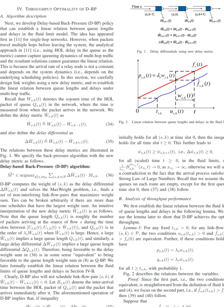
Next, we evaluate the throughput of different schedulers in a grid network that consists of 16 nodes and 24 links as shown in Fig. 4(a), where nodes and links are represented by circles and dashed lines, respectively, with link capacity. We establish 9 multi-hop flows that are represented by arrows. Let λ1 = 0.1 and λ2 = 1. At each time slot, there is a file arrival with probability p = 0.01 for flow (11 → 10 → 9) (represented by the red thick arrow in Fig. 4(a)), and the file size follows Poisson distribution with mean rate5 ρλ
1/p. Note that flow (11→10→9) has bursty arrivals with a small mean rate (we simply call it the bursty flow in the following part). All the other 8 flows have packet arrivals following Poisson 5Note that given the network topology, it is hard to find the exact boundary
of the optimal throughput region of scheduling policies in a closed form. Hence, we probe the boundary by scaling the amount of traffic. After we choose~λ, which determines the direction of traffic load vector, we run our simulations with traffic loadρ~λchanging ρ, which scales the traffic loads.
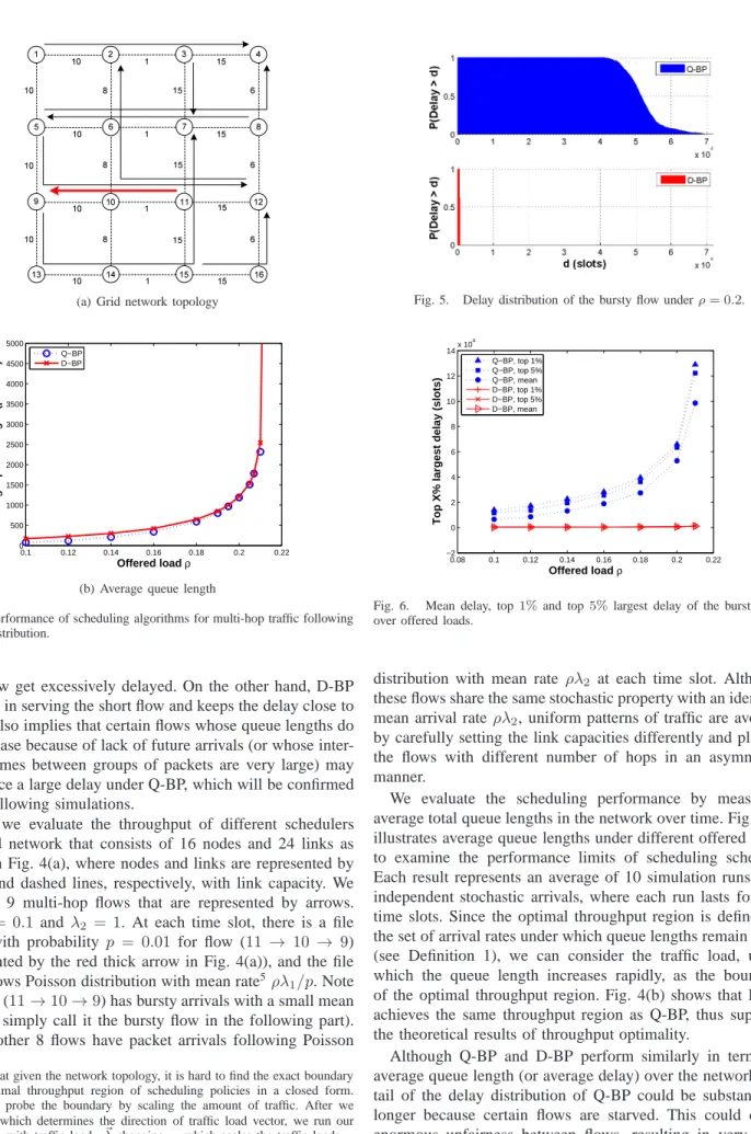
Fig. 5. Delay distribution of the bursty flow underρ= 0.2.
0.08 0.1 0.12 0.14 0.16 0.18 0.2 0.22 −2 0 2 4 6 8 10 12 14x 10 4 Offered load ρ
Top X% largest delay (slots)
Q−BP, top 1% Q−BP, top 5% Q−BP, mean D−BP, top 1% D−BP, top 5% D−BP, mean
Fig. 6. Mean delay, top1%and top5%largest delay of the bursty flow over offered loads.
distribution with mean rate ρλ2 at each time slot. Although these flows share the same stochastic property with an identical mean arrival rateρλ2, uniform patterns of traffic are avoided by carefully setting the link capacities differently and placing the flows with different number of hops in an asymmetric manner.
We evaluate the scheduling performance by measuring average total queue lengths in the network over time. Fig. 4(b) illustrates average queue lengths under different offered loads to examine the performance limits of scheduling schemes. Each result represents an average of 10 simulation runs with independent stochastic arrivals, where each run lasts for 106 time slots. Since the optimal throughput region is defined as the set of arrival rates under which queue lengths remain finite (see Definition 1), we can consider the traffic load, under which the queue length increases rapidly, as the boundary of the optimal throughput region. Fig. 4(b) shows that D-BP achieves the same throughput region as Q-BP, thus supports the theoretical results of throughput optimality.
Although Q-BP and D-BP perform similarly in terms of average queue length (or average delay) over the network, the tail of the delay distribution of Q-BP could be substantially longer because certain flows are starved. This could cause enormous unfairness between flows, resulting in very poor
QoS for certain flows. Note that although a bursty flow is a long flow that has an infinite amount of data, the arrivals occur in a dispersed manner (i.e., the inter-arrival times between groups of packets are very large) and we can view this bursty flow as consisting of many short flows. Thus, we expect that the bursty flow may experience a very large delay under Q-BP due to lack of subsequent packet arrivals over long periods of time that does not allow the queue-lengths to grow and thus contributes to the long tail of the delay distribution. However, this phenomenon may not manifest itself in terms of a higher average delay for Q-BP, as can be observed in Fig. 4(b), because the amount of data corresponding to the bursty flow in the simulation is small compared to the other flows. On the other hand, D-BP can achieve better fairness by scheduling the links based on delays and not starving bursty or variable flows. We confirm this in the following observations.
We now illustrate the effectiveness of using D-BP over Q-BP in terms of how each scheme affects the delay distribution of bursty flows. We plot the delay distribution of the bursty flow in Fig. 5 under ρ = 0.2. It reveals that the tail of the delay distribution under D-BP vanishes much faster than Q-BP. Further, we plot the mean delay, top6 1% and top 5% largest delays of the bursty flow over offered loads in Fig. 6. All these delays under D-BP are substantially less than under Q-BP, which implies that D-BP successfully eliminates the excessive packet delays. The top 0.1% largest delays of the whole network demonstrate similar behaviors in Fig. 6 and the results are omitted. This confirms that, Q-BP causes a substantially long tail for the delay distribution of the network due to the starvation of the bursty flow, while D-BP overcomes this and achieves better fairness among the flows by scheduling the links based on delays.
VI. CONCLUSION
In this paper, we develop a throughput-optimal delay-based back-pressure scheme for multi-hop wireless networks. We introduce a new delay metric suitable for multi-hop traffic and establish a linear relation between queue lengths and delays in the fluid limit model, which plays a key role in the performance analysis and proof of throughput-optimality. Delay-based schemes provide a simple way around the well-known last packet problem that plagues the queue-length-based schedulers, and avoid flow starvation. As a result, the excessively long delays that could be experienced by certain flows under the queue-length-based scheduling schemes are eliminated without any loss of throughput.
REFERENCES
[1] L. Tassiulas and A. Ephremides, “Stability properties of constrained queueing systems and scheduling policies for maximum throughput in multihop radio networks,” IEEE Transactions on Automatic Control, vol. 37, no. 12, pp. 1936–1948, 1992.
6Suppose there areNpackets sorted by their delays from the largest to the
smallest, the topX%largest delay is defined as the delay of the⌊N X
100⌋-th
packet. If N X
100 ≤1, it means the maximum delay. For example, if the delays
are[3,2,1,1,1], the top20%largest delay is 2.
[2] X. Lin, N. Shroff, and R. Srikant, “A tutorial on cross-layer optimization in wireless networks,” Selected Areas in Communications, IEEE Journal on, vol. 24, no. 8, pp. 1452–1463, Aug. 2006.
[3] A. Warrier, S. Janakiraman, S. Ha, and I. Rhee, “DiffQ: Practical differential backlog congestion control for wireless networks,” in Proc. of INFOCOM, 2009.
[4] A. Sridharan, S. Moeller, and B. Krishnamachari, “Implementing Backpressure-based Rate Control in Wireless Networks,” in Information Theory and Applications Workshop, 2009.
[5] P. van de Ven, S. Borst, and S. Shneer, “Instability of MaxWeight Scheduling Algorithms,” in Proc. IEEE INFOCOM, 2009, pp. 1701– 1709.
[6] S. Liu, L. Ying, and R. Srikant, “Throughput-Optimal Opportunistic Scheduling in the Presence of Flow-Level Dynamics,” in Proc. IEEE INFOCOM, 2010.
[7] ——, “Scheduling in multichannel wireless networks with flow-level dy-namics,” ACM SIGMETRICS Performance Evaluation Review, vol. 38, no. 1, pp. 191–202, 2010.
[8] A. Mekkittikul and N. McKeown, “A starvation-free algorithm for achieving 100% throughput in an input-queued switch,” in Proc. of the IEEE International Conference on Communication Networks, 1996. [9] M. Andrews, K. Kumaran, K. Ramanan, A. Stolyar, P. Whiting, and
R. Vijayakumar, “Providing quality of service over a shared wireless link,” IEEE Communications magazine, vol. 39, no. 2, pp. 150–154, 2001.
[10] S. Shakkottai and A. Stolyar, “Scheduling for multiple flows sharing a time-varying channel: The exponential rule,” Translations of the American Mathematical Society-Series 2, vol. 207, pp. 185–202, 2002. [11] M. Andrews, K. Kumaran, K. Ramanan, A. Stolyar, R. Vijayakumar, and P. Whiting, “Scheduling in a queuing system with asynchronously varying service rates,” Probability in the Engineering and Informational Sciences, vol. 18, no. 02, pp. 191–217, 2004.
[12] B. Sadiq and G. de Veciana, “Throughput optimality of delay-driven MaxWeight scheduler for a wireless system with flow dynamics,” in Forty-seventh Annual Allerton Conference on Communication, Control, and Computing, Allerton House, Monticello, IL, 2009.
[13] M. Neely, “Delay-based network utility maximization,” in Proc. IEEE INFOCOM, 2010.
[14] A. Eryilmaz, R. Srikant, and J. Perkins, “Stable scheduling policies for fading wireless channels,” IEEE/ACM Transactions on Networking, vol. 13, no. 2, p. 424, 2005.
[15] J. Dai, “On positive Harris recurrence of multiclass queueing networks: a unified approach via fluid limit models,” The Annals of Applied Probability, pp. 49–77, 1995.
[16] A. Rybko and A. Stolyar, “Ergodicity of stochastic processes describing the operation of open queueing networks,” Problems of Information Transmission, vol. 28, no. 3, pp. 3–26, 1992.
[17] V. Malyshev and M. Menshikov, “Ergodicity, continuity and analyticity of countable Markov chains,” Transactions of the Moscow Mathematical Society, vol. 39, pp. 3–48, 1979.
[18] B. Ji, C. Joo, and N. Shroff, “Delay-Based Back-Pressure Scheduling in Multi-Hop Wireless Networks,” November 2010. [Online]. Available: http://arxiv.org/abs/1011.5674
[19] C. Joo, X. Lin, and N. Shroff, “Understanding the capacity region of the greedy maximal scheduling algorithm in multi-hop wireless networks,” in IEEE INFOCOM, 2008, pp. 1103–1111.
[20] ——, “Greedy Maximal Matching: Performance Limits for Arbitrary Network Graphs Under the Node-exclusive Interference Model,” IEEE Transactions on Automatic Control, 2009.
[21] X. Wu, R. Srikant, and J. Perkins, “Scheduling Efficiency of Distributed Greedy Scheduling Algorithms in Wireless Networks,” IEEE Transac-tions on Mobile Computing, pp. 595–605, 2007.
[22] M. Leconte, J. Ni, and R. Srikant, “Improved bounds on the throughput efficiency of greedy maximal scheduling in wireless networks,” in MobiHoc ’09. New York, NY, USA: ACM, 2009, pp. 165–174. [23] C. Joo and N. Shroff, “Performance of random access scheduling
schemes in multi-hop wireless networks,” in IEEE INFOCOM, 2007, pp. 19–27.