Structural damage detection using signal-based pattern recognition

(1)

STRUCTURAL DAMAGE DETECTION USING SIGNAL-BASED PATTERN RECOGNITION

by

LONG QIAO

B.S., Xian University of Architecture and Technology, China, 1998 M.S., Texas Tech University, Lubbock, 2003

AN ABSTRACT OF A DISSERTATION

submitted in partial fulfillment of the requirements for the degree

DOCTOR OF PHILOSOPHY

Department of Civil Engineering College of Engineering

KANSAS STATE UNIVERSITY Manhattan, Kansas

(2)

Abstract

Civil structures are susceptible to damages over their service lives due to aging,

environmental loading, fatigue and excessive response. Such deterioration significantly affects the performance and safety of structure. Therefore, it is necessary to monitor the structural performance, detect and assess damages at the earliest possible stage in order to reduce the life-cycle cost of structure and improve its reliability. Over the last two decades, extensive research has been conducted on structural health monitoring and damage detection.

In this study, a signal-based pattern-recognition method was applied to detect structural damages with a single or limited number of input/output signals. This method is based on the extraction of sensitive features of the structural response under a known excitation that present a unique pattern for any particular damage scenario. Frequency-based features and

time-frequency-based features of the acceleration response were extracted from the measured

vibration signals by Fast Fourier Transform (FFT) and Continuous Wavelet Transform (CWT) to form one-dimensional or two-dimensional patterns, respectively. Three pattern recognition algorithms were investigated when performing pattern-matching: (1) correlation, (2) least square distance, and (3) Cosh spectral distance.

To demonstrate the validity and accuracy of the method, numerical and experimental studies were conducted on a simple small-scale three-story steel building. In addition, the efficiency of the features extracted by Wavelet Packet Transform (WPT) was examined in the experimental study. The results show that the features of the signal for different damage

scenarios can be uniquely identified by these transformations. Suitable correlation algorithm can then be used to identify the most probable damage scenario. The proposed method is suitable for structural health monitoring, especially for the online monitoring applications. Meanwhile, the choice of wavelet function affects the resolution of the detection process and is discussed in the “experimental study part” of this report.

(3)

STRUCTURAL DAMAGE DETECTION USING SIGNAL-BASED PATTERN RECOGNITION

by

LONG QIAO

B.S., Xian University of Architecture and Technology, China, 1998 M.S., Texas Tech University, Lubbock, 2003

A DISSERTATION

submitted in partial fulfillment of the requirements for the degree

DOCTOR OF PHILOSOPHY

Department of Civil Engineering College of Engineering

KANSAS STATE UNIVERSITY Manhattan, Kansas

2009

Approved by: Major Professor Asad Esmaeily

(4)

Copyright

LONG QIAO

(5)

Abstract

Civil structures are susceptible to damages over their service lives due to aging,

environmental loading, fatigue and excessive response. Such deterioration significantly affects the performance and safety of structure. Therefore, it is necessary to monitor the structural performance, detect and assess damages at the earliest possible stage in order to reduce the life-cycle cost of structure and improve its reliability. Over the last two decades, extensive research has been conducted on structural health monitoring and damage detection.

In this study, a signal-based pattern-recognition method was applied to detect structural damages with a single or limited number of input/output signals. This method is based on the extraction of sensitive features of the structural response under a known excitation that present a unique pattern for any particular damage scenario. Frequency-based features and

time-frequency-based features of the acceleration response were extracted from the measured

vibration signals by Fast Fourier Transform (FFT) and Continuous Wavelet Transform (CWT) to form one-dimensional or two-dimensional patterns, respectively. Three pattern recognition algorithms were investigated when performing pattern-matching: (1) correlation, (2) least square distance, and (3) Cosh spectral distance.

To demonstrate the validity and accuracy of the method, numerical and experimental studies were conducted on a simple small-scale three-story steel building. In addition, the efficiency of the features extracted by Wavelet Packet Transform (WPT) was examined in the experimental study. The results show that the features of the signal for different damage

scenarios can be uniquely identified by these transformations. Suitable correlation algorithm can then be used to identify the most probable damage scenario. The proposed method is suitable for structural health monitoring, especially for the online monitoring applications. Meanwhile, the choice of wavelet function affects the resolution of the detection process and is discussed in the “experimental study part” of this report.

(6)

List of Figures

Figure 1.1 SHM and Damage Detection Categories... 1

Figure 3.1 Butterfly... 38

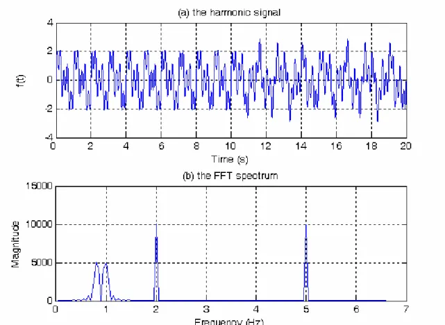
Figure 3.2 The Harmonic Signal and Its FFT Spectrum... 39

Figure 3.3 The Morlet Wavelet... 41

Figure 3.4 Fourier Transform, H(ω) of the Morlet Wavelet... 42

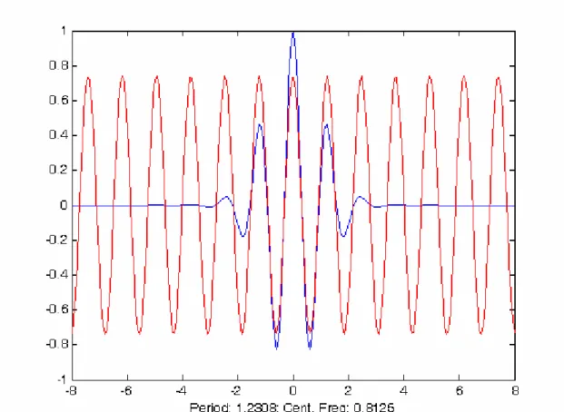
Figure 3.5 Signal f(t) along with the Morlet Wavelet (denoted by w) at Three Scales and Shifts44 Figure 3.6 Wavelet Morlet (blue) and Center Frequency Based Approximation... 45

Figure 3.7 CWT Scale-Space (time) Contours of Signal, f(t)... 46

Figure 3.8 CWT Frequency-Time Contour of Signal, f(t)... 47

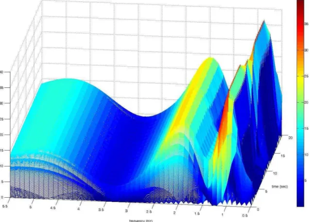
Figure 3.9 3-D View of CWT Frequency-Time Contour of Signal, f(t)... 48

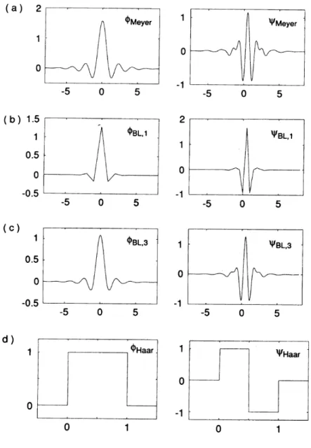
Figure 3.10 Some Example of Pairs of Functions φ, ψ: (a) The Meyer Wavelets; (b) and (c) Battle-Lemarie Wavelets; (d) The Haar Wavelet (Daubechies, 1992) ... 51

Figure 3.11 Three-Level Wavelet Decomposition Tree ... 52

Figure 3.12 Splitting the Signal with an Iterated Filter Bank ... 52

Figure 3.13 Three-Level Wavelet Reconstruction Tree ... 53

Figure 3.14 Decompose Signal at Depth 3 with Discrete Wavelet... 54

Figure 3.15 Tree Structure for Wavelet Packet Analysis ... 57

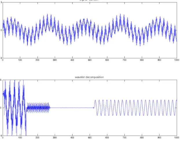
Figure 3.16 Components of the 3rd Level WPT for the Harmonic signal, f (t)... 57

Figure 4.1 Flowchart of Pattern Recognition... 61

Figure 4.2 3-D Steel Structure and 2-D FE Model ... 62

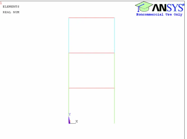
Figure 4.3 2-D Model in ANSYS Graphical User Interface... 63

Figure 4.4 Element Geometric Properties (Real Constants) Screen ... 64

Figure 4.5 Load Steps and Time Steps ... 67

Figure 4.6 Apply F/M on Nodes Window ... 67

Figure 4.7 Time and Time Steps Options Window ... 68

(10)

Figure 4.10 Define Nodal Data Window ... 69

Figure 4.11 Derivative of Time-History Variables Window ... 70

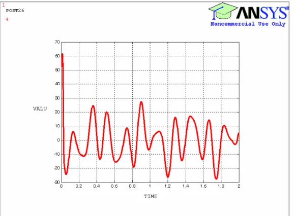
Figure 4.12 Time History Variables Window... 70

Figure 4.13 Acceleration Signal for Baseline Condition (Damage Case 0-0-0)... 71

Figure 4.14 FFT Spectrums for Different Damage Case: (a) Damage Case 0-0-0 (Baseline Condition), (b) Damage Case 20-40-60, (c) Damage Case 20-40, (d) Damage Case 60-60-60 ... 72

Figure 4.15 CWT Contours for Different Damage Cases: (a) Damage Case 0-0-0 (Baseline Condition), (b) Damage Case 40-60, (c) Damage Case 40-60, (d) Damage Case 60-60-60 ... 74

Figure 4.16 FFT Pattern Database 3-D Graph ... 75

Figure 4.17 Acceleration Signals for Damage Case 0-38-38 ... 78

Figure 5.1 Test Three-Story Steel Structure ... 82

Figure 5.2 Slab and Flat Bar Connection... 83

Figure 5.3 Slab and Flat Bar Connection... 84

Figure 5.4 Foundation Slab Fixing ... 84

Figure 5.5 Close View of Magnetic Base, Ball, Chain and Frame ... 86

Figure 5.6 [Left] Relative High level Impulse Force Applicator; [Right] Relative low level Impulse Force Applicator... 87

Figure 5.7 Structure Acceleration Signals Caused by Two Different Level Excitations ... 88

Figure 5.8 Normalized FFT Spectrums of Structure Accelerations by Two Different Level Impulse Excitations... 89

Figure 5.9 Normalized CWT Contours of Structure Response under Different Level Impulse Excitations... 90

Figure 5.10 G-Link and Its Physical Axis Orientation ... 91

Figure 5.11 USB Base Station ... 92

Figure 5.12 Agile-LinkTM software interface... 93

Figure 5.13 G-Link Configuration Screen ... 93

Figure 5.14 Installation of the G-Link ... 95

Figure 5.15 Damage Simulation on experimental structure ... 95

(11)

Figure 5.17 Experimental Acceleration Signals of Structure under Damage Case 20-20-40,

Original and De-noised ... 100

Figure 5.18 Correlation Matching for Damage Case 0-0-20, FFT & CWT Pattern Matching... 103

Figure 5.19 Least Square Distance (LSD) Matching for Damage Case 0-0-20, FFT & CWT Pattern Matching ... 104

Figure 5.20 Cosh Spectral Distance (CSD) Matching for Damage Case 0-0-20, FFT & CWT Pattern Matching ... 105

Figure 5.21 Correlation Matching for Damage Case 0-0-20, WPT Pattern Matching ... 106

Figure B.1 Correlation Matching for Damage Case 19-0-0 (FFT Pattern Database) ... 127

Figure B.2 Correlation Matching for Damage Case 0-38-38 (FFT Pattern Database) ... 130

Figure B.3 Correlation Matching for Damage Case 58-38-19 (FFT Pattern Database)... 132

Figure B.4 Correlation Matching for Damage Case 58-58-58 (FFT Pattern Database)... 134

Figure B.5 Least Square Distance (LSD) Matching for Damage Case 19-0-0 (FFT Pattern Database)... 136

Figure B.9 Cosh Spectral Distance (CSD) Matching for Damage Case 19-0-0 (FFT Pattern Database)... 144

Figure B.10 Cosh Spectral Distance (CSD) Matching for Damage Case 0-38-38 (FFT Pattern Database)... 146 Figure B.11 Cosh Spectral Distance (CSD) Matching for Damage Case 58-38-19 (FFT Pattern

(12)

Figure B.12 Cosh Spectral Distance (CSD) Matching for Damage Case 58-58-58 (FFT Pattern

Database)... 150

Figure B.13 Correlation Matching for Damage Case 19-0-0 (CWT Pattern Database) ... 152

Figure B.17 Least Square Distance (LSD) Matching for Damage Case 19-0-0 (CWT Pattern Database)... 160

Figure B.20 Least Square Distance Matching for Damage Case 58-58-58 (CWT Pattern Database)... 166

Figure B.21 Cosh Spectral Distance (CSD) Matching for Damage Case 19-0-0 (CWT Pattern Database)... 168

Figure B.22 Cosh Spectral Distance Matching for Damage Case 0-38-38 (CWT Pattern Database)... 170

Figure D.1 Correlation Matching for Damage Case 0-20-0, FFT & CWT Pattern Matching.... 181

Figure D.2 Least Square Distance (LSD) Matching for Damage Case 0-20-0, FFT & CWT Pattern Matching ... 183

Figure D.3 Cosh Spectral Distance (CSD) Matching for Damage Case 0-20-0, FFT & CWT Pattern Matching ... 184

Figure D.4 Correlation Matching for Damage Case 20-0-0, FFT & CWT Pattern Matching.... 185

Figure D.5 Least Square Distance (LSD) Matching for Damage Case 20-0-0, FFT & CWT Pattern Matching ... 186

(13)

Figure D.6 Cosh Spectral Distance (CSD) Matching for Damage Case 20-0-0, FFT & CWT Pattern Matching ... 187 Figure D.7 Correlation Matching for Damage Case 0-20-20, FFT & CWT Pattern Matching.. 188 Figure D.8 Least Square Distance (LSD) Matching for Damage Case 0-20-20, FFT & CWT

Matching ... 189 Figure D.9 Cosh Spectral Distance (CSD) Matching for Damage Case 0-20-20, FFT & CWT

Pattern Matching ... 190 Figure D.10 Correlation Matching for Damage Case 20-0-20, FFT & CWT Pattern Matching 191 Figure D.11 Least Square Distance (LSD) Matching for Damage Case 20-0-20, FFT & CWT

Pattern Matching ... 192 Figure D.12 Cosh Spectral Distance (CSD) Matching for Damage Case 20-0-20, FFT & CWT

Pattern Matching ... 199 Figure D.19 Correlation Matching for Damage Case 20-20-20, FFT & CWT Pattern Matching

... 200 Figure D.20 Least Square Distance (LSD) Matching for Damage Case 20-20-20, FFT & CWT

(14)

Figure D.23 Least Square Distance (LSD) Matching for Damage Case 20-20-40, FFT & CWT Pattern Matching ... 204 Figure D.24 Cosh Spectral Distance (CSD) Matching for Damage Case 20-20-40, FFT & CWT

... 206 Figure D.26 Least Square Distance (LSD) Matching for Damage Case 40-60-20, FFT & CWT

(15)

List of Tables

Table 4.1 Peak Values on the FFT Spectrums ... 73

Table 4.2 Numerical Test Cases ... 76

Table 4.3 Signal Properties ... 77

Table 4.4 FFT and CWT Pattern Recognition Results ... 80

Table 5.1 Dimensions, Weights and Amount of Structure Components ... 82

Table 5.2 G-Link Specifications ... 91

Table 5.3 3-D FE Model Baseline Properties ... 97

Table 5.4 Experimental Test Cases... 99

(16)

Acknowledgements

I would like to express my deepest and sincerest gratitude to my major professor Dr. Asad Esmaeily. I also express my appreciation for the support received from Dr. Hani G. Melhem. Their knowledge, insight, patience and encouragement have been highly appreciated.

I would also like to thank Dr. Jacob Najjar and Dr. Jack Xin for serving on my committee and Dr. David Schmidt for being the outside committee chair. Their advice and support are highly appreciated. I would also like to thank Mr. Dave Suhling, a research technologist in Civil Engineering Lab, for providing assistance during construction and testing of the experimental structure.

This work was financially supported by Dr. Esmaeily’s start up funds provided by Kansas State University, Engineering Experimental Station, through the pertinent contract. I would like to acknowledge and express my thanks for the opportunity that made this work possible.

(17)

Dedication

This work is dedicated to my parents and my wife for their encouragement, patience, support, and love.

(18)

CHAPTER 1 - INTRODUCTION

1.1 Introduction

Deterioration of structures due to aging, cumulative crack growth or excessive response decreases their stiffness and integrity, and therefore significantly affects the performance and safety of structures during their service life. Structural Health Monitoring (SHM) and damage detection denotes the ability to monitor the performance of structure, detect and assess any damage at the earliest stage in order to reduce the life-cycle cost of structure and improve its reliability and safety. Figure 1.1 shows a brief classification of different damage detection categories, methods and basic algorithms.

(19)

In this field, Destructive Damage Detection (DDD) and/or Non-destructive Damage Detection (NDD) techniques are employed to continuously monitor the structure, detect the possible damage, and evaluate the safety of the structure. Recent advances in computer, sensors and other electronic technologies make NDD techniques far more convenient and cost effective than destructive detection techniques which usually evaluate the safety of a structure by testing samples removed from the structure. NDD techniques can be classified into two categories: (1) local methods; and (2) global methods.

Current highly effective localized NDD methods include acoustic or ultrasonic methods, magnetic field methods, radiograph, microwave/ground penetrating radar, fiber optics, eddy-current methods and thermal field methods. These methods are visual or localized experimental methods that detect damage on or near the surface of the structure by measuring light, sound, electromagnetic field intensity, displacements, or temperature. Some of these methods are particularly effective for a specific application. For example, eddy current is very effective for crack detection at welded joint (Chang and Liu, 2003). But these methods have several

limitations when testing large and complex structures. First, the depth of wave penetration is limited. Second, the vicinity of the damage should be known and the portion of the structure being inspected should readily be accessible. However, there is no easy way to determine the global health condition of a structure. Chang and Liu (2003) provided detailed information about “local” methods.

Static-based and vibration-based NDD methods provide the opportunity to detect and assess damage on a global basis. Static-based methods rely on the strain or displacement measurements from a structure under known static loads and the finite-element model updating to determine changes in deflection, stiffness, and load-carrying capacity of the structure. These methods are widely used for bridge health monitoring and evaluation. Examples of such work are Barr et al. (2006) and Cardinale and Orlando (2004). The drawbacks of static-based NDD methods are: (1) they require a large amount of measured data; (2) they require the finite-element model updating using accurate material properties; (3) they require static-load tests which will interrupt the structure service. These drawbacks will make static-based NDD methods more difficult for online damage detection of an in-service structure. Vibration-based NDD methods rely on the change of vibration characteristics and signals as indication of damage due to the

(20)

changes to the vibration characteristics and signals of the structure. Over the last two decades, extensive research has been conducted on Vibration-based detection approach, leading to various experimental techniques, methodologies, and signal processing algorithms. Doebling et al. (1996) and Sohn et al. (2003) presented comprehensive literature reviews of vibration based damage detection and health monitoring methods for structural and mechanical systems. These methods can be classified into either modal-based or signal-based categories.

Modal-based methods use changes in measured modal parameters (resonant frequencies, modal damping, mode shapes, etc.) or their derivatives as a sign of change in physical-dynamic properties of the structure (stiffness, mass and damping). The basic premise behind the methods is that a change in stiffness leads to a change in natural frequencies and mode shapes. Modal-based methods have been applied successfully to identify the dynamic properties of linearized and time-invariant equivalent structural systems. The methods include mode shape curvature method, the change in flexibility method, the change in stiffness method, modal strain energy, etc. Examples of such work are Kosmatka and Ricles (1999), Ren and Roeck (2002), Shi et al. (2000) and Kim et al. (2003). Recently, wavelet-based and Hilbert-based approaches have been developed as enhanced techniques for parametric identification of non-linear and time-variant systems. Examples of such work are Staszewski (1998), Kijewski and Kareem (2003), Yang et al. (2004), Huang et al. (2005), Hou et al. (2006), Chen et al. (2006) and Yan and Miyamoto (2006). Although modal-based methods are generally applicable for the purpose of damage detection and structural health monitoring, they still have many problems and challenges: (1) damage is a local phenomenon and may not significantly influence modal parameters,

particularly for large structures; (2) variation in the mass of the structure or environmental noise may also introduce uncertainties in the measured modal parameters; (3) the number of sensors, the types of sensors, and the coordinates of sensors may have a crucial effect on the accuracy of the damage detection procedure (Kim et al. 2003).

Signal-based methods examine changes in the features derived directly from the

measured time histories or their corresponding spectra through proper signal processing methods and algorithms to detect damage. Based on different signal processing techniques for feature extraction, these methods are classified into time-domain methods, frequency-domain methods, and time-frequency (or time-scale)-domain methods. Time-domain methods use linear and nonlinear functions of time histories to extract the signal features. Examples of this category are

(21)

Regressive (AR) model, Regressive Moving Average (ARMA) model,

Auto-Regressive with eXogenous input (ARX) model and Extended Kalman Filter (EKF). Frequency-domain methods use Fourier analysis and cepstrum (the inverse Fourier transform of the

logarithm of the Fourier spectra magnitude squared) analysis to extract features in a given time window. Examples of this category are Frequency Response Functions (FRFs), frequency spectra, cross power spectra, power spectra, and power spectral density. Time-frequency domain methods employ Wigner-Ville distribution and wavelet analysis to extract the signal features. Examples of this category are spectrogram, continuous wavelet transform coefficients, wavelet packet energies and wavelet entropy. Detailed descriptions of these signal-based features, feature extraction and successful applications will be presented in Chapter Two. As an

enhancement for feature extraction, selection and classification, pattern recognition techniques are deeply integrated into signal-based damage detection. Staszewski (2000) and Farrar et al. (2001) presented the detailed descriptions of feature extraction, selection and analysis in the context of statistical pattern recognition. Some cases of successful application of the procedure for damage detection can be found in Sohn et al. (2000, 2001), Trendafilova (2001), Posenato et al. (2008) and Fang et al. (2005). Detailed descriptions of these mostly used pattern recognition methods and successful applications for damage detection will also be presented in Chapter Two. Compared with modal-based methods, signal-based methods have received considerable

attentions from the civil, aerospace, and mechanical communities because they are particularly more effective for structures with complicated nonlinear behavior and the incomplete,

incoherent, and noise-contaminated measurements of structural response (Adeli and Jiang 2006). They are also more cost effective and suitable for online structural monitoring.

1.2 Objectives

The overall problem of structural damage detection involves five levels of damage identification which are categorized according to a logical sequence: level 1, existence of damage; level 2, location of damage; level 3, type of damage; level 4, quantity of the damage; and level 5, life to failure (Sohn et al. 2003, Doebling et al. 1996, Rytter 1993). The first four levels are mostly related to identification and modeling of structural systems, signal processing, feature extraction and statistical pattern recognition. The last level of identification generally

(22)

falls into the fields of fatigue life analysis, fracture mechanics, design assessment, reliability analysis and machine learning.

The main goal of any damage detection method is to detect the damage, assess the level and type, and spot the location. As detailed in the introduction, there are many methods and algorithms that can be used depending on the type of structure, source of possible damage and the desired accuracy of detection.

The method used in this study is a signal-based method in which the features of the acceleration response signal, under a known excitation serve as the structural signature. This signature will change when the dynamic properties of the structure changes due to an inflicted damage that will alter the dynamic properties of the structure.

The main goal of this study was to: (1) explore various signal processing methods in optimal extraction and preservation of the features of the response signal; (2) identify the best pattern recognition method; (3) develop a process of pattern extraction and recognition for damage detection and online structural monitoring.

In this study, a signal-based pattern extraction and recognition method, using a number of signal transformations and pattern matching algorithms, was investigated to detect structural damage. The vibration acceleration signals of a structure excited by a known dynamic excitation, such as an impulse force, were decomposed by Fast Fourier Transform (FFT), Continuous Wavelet Transform (CWT) or Wavelet Packet Transform (WPT) for feature extraction. Three statistical algorithms were also investigated to perform pattern matching separately: correlation, least square distance, and Cosh spectral distance. The method proposed in this study implements feature extraction and pattern recognition algorithms in damage detection procedure. To show the validity and accuracy of the method and related

transformation and pattern recognition algorithms, numerical simulation and experimental case studies were conducted on a small-scale three-story steel structure. The structural dynamic response under different damage scenarios excited by an impulsive load was numerically

simulated by a detailed finite element model using ANSYS, and the recorded vibration response was processed using MATLAB.

(23)

CHAPTER 2 - LITERATURE REVIEW

Recently, signal-based damage detection methods have received many attentions. These methods involve two main processes: (1) feature extraction and selection, and (2) pattern

recognition. Feature extraction and selection is the process of identifying and selecting damage-sensitive features derived from the measured dynamic response, to quantify the damage state of the structure (Sohn et al. 2003). This process often involves fusing and condensing the large amount of available data from multiple sensors into a much smaller data set that can be better analyzed in a statistical manner. Also, various forms of data normalization are employed in the process in an effort to separate changes in the measured response caused by varying operational and environmental condition from changes caused by damage.

A pattern can be a set of features given by continuous, discrete or discrete-binary variables formed in vector or matrix notation. “Pattern recognition is concerned with the implementation of the algorithms that operate on the extracted features and unambiguously determine the damage state of the structure” (Farrar et al. 2001).

2.1 Feature Extraction and Selection

A variety of methods are employed to improve the feature extraction and selection procedure. Based on different signal processing techniques for feature extraction, these methods are classified into time-domain methods, frequency-domain methods, and time-frequency

methods.

2.1.1 Time-domain Methods

Time-domain methods use linear and nonlinear functions of time histories to extract features. Sohn et al. (2000) used an auto-regressive (AR) model to fit the measured time history on a structure. Damage diagnoses using X-bar control chart were performed using AR

coefficients as damage-sensitive features. In the AR n model, the current point in a time series

( )

(24)

( )

(

)

( )

1 n j x j x t x t j e t = =

∑

φ − + (2.1) where x t is the time history at time t;

( )

φ_j is the unknown AR coefficient; and e t is the _x

( )

random error with zero mean and constant variance. The value of φ_j is estimated by fitting the AR model to the time history data. The AR coefficients of the model fit to subsequent new data were monitored relative to the baseline AR coefficients. The X-bar control chart was used to provide a framework for monitoring the changes in the mean values of the AR coefficients and identifying samples that were inconsistent with the past data sets. A statistically significant number of AR coefficients outside the control limits indicated that the system was transited from a healthy state to a damaged state. Principal component analysis and linear and quadratic

projections were applied to transform the time series from multiple measurement points into a single time series in an effort to reduce the dimensionality of the data and enhance the

discrimination between features from undamaged and damaged structures. For demonstration, the authors applied the AR model combined with X-bar control chart to determine the existence of damage on a concrete bridge column as the column was progressively damaged. The AR coefficients on the X-bar control chart as detailed in the method indicated the damage existence.

Sohn and Farrar (2001) proposed a two-stage time history prediction model, combining auto-regressive (AR) model and an autoregressive with exogenous inputs (ARX) model. The residual error, which was the difference between the actual acceleration measurement for the new signal and the prediction obtained from the AR-ARX model from the reference signal, was defined as the damage-sensitive feature. The increase in residual errors was monitored to detect system anomalies. In this method, the ARX model is expressed as

( )

(

)

( )

1 1 a b i j x x i j x t x t i e t j t = = ∑ ∑ = α − + β − + ε (2.2) where a and b are the order of the ARX model; αi and βj are the coefficients of the AR and the

exogenous input, respectively; ε_x

( )

t is the residual error after fitting theARX a,b model to

( )

the e t and _x

( )

x t pair in the one-stage ahead AR model. If the ARX model obtained from the

( )

reference signal block pair x t and

( )

e t were not be a good representation of the newly x

( )

(25)

( )

y t

ε , compared to εx

( )

t . The standard deviation ratio of the residual errors,σ ε

( )

y σ ε

( )

x ,

would reach its maximum value at the sensors instrumented near the actual damage locations. The applicability of this approach was demonstrated by the authors using acceleration time histories obtained from an eight degree-of-freedom mass-spring system.

Sohn et al. (2002) developed a unique combination of the AR-ARX model, auto-associative neural network, and statistical pattern recognition techniques for damage

classification explicitly taking the environmental and operational variations of the system in the consideration. In this method, AR-ARX model is developed to extract damage sensitive

features, which are theα_i and β_j coefficients of the ARX model. An auto-associative neural network is trained to characterize the dependency of the extracted features on the variations caused by environmental and operation conditions. A damage classifier is constructed using a sequential probability ratio test to automatically determine the damage condition of the system. The authors demonstrated the proposed approach using a numerical example of a computer hard disk and an experimental study of an eight degree-of-freedom spring-mass system.

Bodeux and Golinval (2001) applied the autoregressive moving average vector

(ARMAV) model and statistical tools such as confidence interval and the normal distribution of random variable for damage detection. In the state space, the ARMAV model is expressed as

[ ]

1

[ ]

x n =Ax n− +W n (2.3) where x n is the observed vibration vector at the nth discrete time point; A is the matrix

[ ]

containing the different coefficients of the autoregressive (AR) part; W n is a matrix containing

[ ]

the moving average (MA) terms. The natural eigenfrequencies f and damping ratios r ζr can be

extracted from the eigenvalues τr of the AR matrix A as

( )

2 ln _r r f t τ = π ∆ (2.4)

( )

(

)

( )

r r Real ln ln r τ ζ = τ (2.5) where t∆ is the discrete time interval. The authors used the changes in the frequencies estimated

(26)

and a negative change in frequencies indicated damage caused by structure change. As damage indicator, the probability of negative change

i f P_δ in frequency fi is given by 0 2 2 0 1 i i i f i i f f P_δ = − Φ −  σ + σ   (2.6)

where σ2_i and σ_i2₀ are the variances of the frequencies f_iand f_i₀corresponding to the damaged and undamaged states. Φ is the unit normal distribution function. The structure was assumed damaged if the probability was close to one. The proposed method was limited to only detecting the damage existence.

Nair et al. (2006) applied an Auto-Regressive Moving Average (ARMA) model for damage identification and localization. A damage-sensitive feature, DSF, was defined as a function of the first three auto regressive (AR) components. The mean values of the DSF obtained from the damaged and undamaged signals were significantly different. In this method, the vibration signals obtained from sensors are modeled as ARMA time series as

(

)

(

)

( )

1 1 p q ij k ij k ij ij k k x x t k t k t = = ∑ ∑ = ϕ − + θ ε − + ε (2.7)

where x_ij

( )

t is the normalized acceleration signal; ϕ_k and θ_k are the k-th AR (Auto-Regressive) and MA (Moving Average) coefficients, respectively; p and q are the model orders of the AR

and MA processes, respectively; and εij

( )

t is the residual term. DSF is defined as

1

2 2 3

1 2 3

DSF = α

α + α + α (2.8)

where α1, α2 and α3 are the first three AR coefficients. A hypothesis test involving the t-test

was used to determine the existence of damages on the structure. Two indices, LI1 and LI2, were

introduced based on the AR coefficient space to localize damages. At the sensor locations where damage was introduced, LI1 and LI2 had comparatively large values. The authors tested the

proposed methodologies on the analytical and experimental results of the ASCE benchmark structure. The results of the damage detection indicated that DSF was able to detect the

existence of all damage patterns in the ASCE Benchmark simulation experiment. The results of the damage localization indicated that LI1 and LI2 were all able to localize minor damages but

(27)

Nair and Kiremidjian (2007) utilized the Gaussian Mixture Model (GMM) to detect the existence and extent of damage. The vibration signals obtained from the structure were modeled as ARMA processes. The first three autoregressive coefficients obtained from the modeling of the vibration signals formed the feature vector. The feature vectors were clustered by Gaussian mixture model. The existence of damage was detected using the gap statistic to ascertain the optimal number of mixtures in a particular database. A migration of the number of mixtures indicated the existence of damage. The Mahalanobis distance between the centroids of the mixture in question and the undamaged mixture was chosen as a good indicator of damage extent. The authors used the simulation data from the ASCE benchmark structure to test the efficacy of the method. It was demonstrated that GMM-based algorithm was able to detect minor, moderate, and major damage patterns; the Mahalanobis distance was highly correlated to the damage extent even under the presence of noise. The limitations of the algorithm were that this algorithm was effective only for linear stationary signals; and changes are identified relative to the initial measurement which was assumed to be the undamaged state.

Liu et al. (2007) presented a damage sensitive feature index for damage detection based on Auto-Regressive Moving Average (ARMA) time series analysis. The acceleration signal was modeled as ARMA models, and a principal component matrix derived from the AR coefficients of these models was utilized to establish the Mahalanobis distance criterion function. The Mahalanobis-distances of m-dimensional vector xi from the principal component matrix of

damaged structure to the ones of undamaged structure were defined as the damage sensitive feature (DSF) index. It is expressed as

(

)

T 1

(

)

12

DSF

D =_ x− µ ∑− x− µ _ (2.9) where µ and ∑ are mathematics expectation and covariance matrices of the m-dimensional vector from the principal component matrix of undamaged structure, respectively. A hypothesis test involving the t-test method was further applied to make a damage alarming decision by determining the statistical significance in the difference of mean values ofDDSF obtained from

the damaged and undamaged cases. These methodologies were tested on a numerical three-span-girder beam model containing some subtle damages. The results show that the defined index is sensitive to these subtle structure damages, and the proposed algorithm can be applied to the

(28)

on-Yan et al. (2004) applied the residual errors of the prediction model and statistical process control techniques for damage diagnosis. A Kalman model was constructed to fit the measured vibration response histories of the undamaged structure. The residual error of the prediction by the identified Kalman model with respect to the actual measurement of signals was defined as a damage-sensitive feature. The X-bar control chart was constructed to provide a quantitative indicator of damage. The damage locations were determined as the errors reached the maximum values at the sensors instrumented in the damaged sub-structures. The authors successfully applied this method to indicate the system anomaly on an aircraft model in a laboratory and on a real bridge.

Omenzetter and Brownjohn (2006) applied the time series analysis to process data from a continuously operating SHM system installed in a major bridge structure. The strain data

recorded during the construction and service life of the bridge were modeled using a vector seasonal autoregressive integrated moving average (ARIMA) model. The model is expressed as

( )

( )S

_{( ) ( )}

( )S

_{( )}

( )S

_{( )}

t t t t t t

D B D B Φ B Φ B x = Θ B Θ B e (2.10) where

{ }

x_t (t = 1, 2… N) is the p-dimensional vector of the time series of analyzed signal;

{ }

e_t is

zero mean multivariate Gaussian white noise; B denotes the backshift operator; Φt

( )

B ,

( )S

_{( )}

t B

Φ , Θt

( )

B , and

( )S

_{( )}

t B

Θ are all matrix polynomials in the backshift operator. The

coefficients of the ARIMA model were identified on-line by an extended Kalman filter and chosen as damage sensitive features. The various changes in the features were statistically examined using an outlier detection technique to reveal unusual events as well as structural change or damage sustained by the structure.

2.1.2 Frequency-domain Methods

Frequency-domain methods analyze any stationary event localized in time domain. They use Fourier analysis, cepstrum (the inverse Fourier transform of the logarithm of the Fourier spectra magnitude squared) analysis, spectral analysis, frequency response technique, etc to extract features in a given time window. Tang et al. (1991) quantitatively diagnosed gear-wear through cepstrum analysis of gear noise signals. The amplitude value of the peak in cepstrum represented gear mesh-harmonics in spectrum. The trend of the change of gear-wear degree was about the same as that of the change of the value of a peak in cepstrum. The value was

(29)

independent of intensity of gear noise signal and was used as an indicator for quantitatively diagnosing gear-wear. Based on analyzing the results of experiments with gearboxes, the thresholds of the gear wear by cepstrum diagnosis was determined to distinguish normal, moderate and serious wears. The theoretical analysis agreed with the experimental results very well.

Kamarthi and Pittner (1997) presented sensor data representation schemes for flank wear estimation in turning processes. The sensor data representation algorithm based on fast Fourier transform (FFT) transformed a time series vector X of the sensor signal from turning experiments

into the spectral vectorɵx, and then formed the vector xɵfwith the set

{

i ,i ,...,i₁ ₂ _d

}

. The

featuresxr, the d-dimensional sensor data representation of X, was computed through the relation

ɵ

1 2/ f

r w

x =S− x (2.11) The features were used by recurrent neural network architecture to continually compute the flank wear estimates.

Lee and Kim (2007) used the frequency analysis to detect and localize damage. A signal anomaly index (SAI) which quantified the change of frequency response was developed as damage feature. The SAI is defined as a Euclidean norm of the difference between two frequency response function (FRFs) of basis and compared state as

( )

1 1 1 2 2 2 B C B FRF FRF FRF n i n i f B C f f i i f B f f i H f H f SAI H f = = ∑ ∑  ₋  ₋   =_ _ =   (2.12)

where, H

( )

and FRF represent the frequency response function in continuous form and

discrete form respectively, superscript B and C stand for the state of Basic and Compared. The symbols, f1 and fn are the lowest and highest frequency of the considering frequency range,

respectively. Changes in the shape of the FRF due to the reason of structural damage caused the increase of SAI value. The presence of damage was identified from the SAI value. All SAI values calculated from different sensors and different frequency ranges formed a SAI matrix which showed variation patterns of the FRF in both the space and the frequency domain. The SAI matrix was used as input for the neural network to identify the location of damage. The authors conducted a series of experimental tests and numerical simulation on an experimental

(30)

example application show that the SAI based pattern recognition approach has the great potential for structural health monitoring on a real bridge.

Fasel et al. (2005) used a frequency domain auto-regressive model with exogenous inputs (ARX) to detect joint damage in steel moment-resisting frame structures. Damage sensitive features were extracted from the ARX model in the consideration of non-linear system

input/output relationships. A frequency domain ARX model was used to predict the response at a particular frequency based on the input at that frequency, as well as responses at surrounding frequencies. The responses at the surrounding frequencies were included as inputs to the model to account for sub-harmonics and super-harmonics introduced to the system through non-linear feedback. To accounts for non-linearity in the system, first-order ARX model in the frequency domain is built as

( )

( ) ( )

1

( ) (

1

)

1

( ) (

1

)

Y k =B k U k +A k Y k− +A₋ k Y k+ k =2 3, ,..., Nf −1 (2.13) where N_f is the highest frequency value examined, Y k

( )

is the response at the k-th frequency,

( )

U k is the input at the k-th frequency, and Y k

(

−1

)

and Y k

(

+1

)

are the responses at the (k-1)th and (k+1)th frequencies, respectively. A k₁

( )

and A₋₁

( )

k are the frequency domain

auto-regressive coefficients, and B k

( )

is the exogenous coefficient. The frequency response of one accelerometer was treated as an input and the other accelerometer response was treated as an output. The auto-regressive coefficients in this frequency domain model were used as features. These features were then analyzed using extreme value statistics (EVS) to differentiate between damage and undamaged conditions. The suitability of the ARX model, combined with EVS, to non-linear damage detection was demonstrated on a three-story building model.

2.1.3 Time-Frequency (or Scale)-domain Methods

In contrast to the frequency-domain methods, the time-frequency (or scale) methods can be used to analyze any non-stationary event localized in time domain. Staszewski et al. (1997) applied the Wigner-Ville distribution (WVD) to detect local tooth faults in spur gears. The authors showed that the visual observation of the WVD contour plots could be used for fault detection. Dark zones and curved bands in the contour plots were the main features of an impulse produced by the fault in the spur gear. The changes in features of the distribution were used to monitor the progression of a fault. For the sake of automatic fault detection, the authors

(31)

chose the two-dimensional contour plots of the WVD as patterns, and the amplitude values of the contour plots as features. Pattern recognition procedures based on the statistical and neural approaches were used for classification of different fault conditions.

Biemans et al. (2001) employed the orthogonal wavelet analysis of the strain data measured from piezoceramic sensors to detect crack growth in the middle of a rectangular aluminum plate. The strain data measured from the plate under the Gaussian white noise

excitation was decomposed into orthogonal wavelet levels. The logarithm of the variance of the

orthogonal wavelet coefficients was calculated for all wavelet levels. The mean vectorµ, of the logarithms for the undamaged plate formed the template for the similarity analysis. A Euclidean

distance between the template µ and the logarithmsx, for the damaged plate was used as a damage index. The damage index is denoted as

( ) ( )

2 T

x ,

d _µ = − µx x− µ (2.14) The mean and standard deviation of the damage index representing the undamaged condition of the plate were used to establish an alarm level. The damage could be considered existence in the plate if the damage index was above the alarm level. The experimental results on the aluminum plate show that such damage index can be used to successfully detect as small as 6-7mm crack and to monitor the crack growth.

Hou et al. (2000) presented the great potential of wavelet analysis for singularity extraction in the signals. Characteristics of four types of representative vibration signals were examined by continuous and discrete wavelet transforms. The singularity in these signals were extracted and best illustrated in the plot of wavelet coefficient in the time-scale plane. The fringe pattern in the continuous wavelet coefficient contour plot indicated the existence of a singularity in the local time and the spike in the discrete wavelet coefficient plot also indicated the existence of a singularity in the local time. The sensitivity of wavelet results to a singularity was

effectively used to detect possible structural damage using measured acceleration response data. To demonstrate the feasibility of the proposed method, the authors used both numerical

simulation data from a simple structural model with multiple paralleled breakable springs and actual acceleration data recorded on the roof of a building during an earthquake event. The detection results showed that occurrence of damage could be detected by spikes in the detailed of

(32)

accurately indicate the moments when the damage occurred. The similar work can also be found on Hera and Hou (2004), Ovanesova and Suarez (2004) and Melhem and Kim (2003, 2004).

Kim and Kim (2005) used the ratio of the incident wave toward and the reflected wave from the damage as index to assess the damage size. The ratio was estimated by the continuous wavelet transform of the measured signal and the ridge analysis. In the time-frequency plane of the continuous wavelet transform, the ridge was traced to compare the magnitude of the incident wave and the magnitude of the reflected wave from the damage. It was found that “the ratio of these magnitudes along the two ridges was the same as the ratio of the magnitude of the incident wave to the magnitude of the reflected wave. Due to the fact that the magnitude and frequency-dependent pattern of the ratio varied with damage size, it was able to correlate the ratio and the damage size except when the damage size was very small” (Kim and Kim 2005). The authors conducted the wave experiments in a cylindrical ferromagnetic beam. Magnetostrictive sensors were used to measure the bending waves in the beam cross section. The continuous Gabor wavelet transform was employed to estimate the crack size in the beam.

Robertson et al. (2002) used the Holder exponent as damage-sensitive to detect the presence of damage and determine the moment of damage occurrence because of its time-varying nature. The authors provided a procedure to capture the time-time-varying nature of the Holder exponent based on wavelet transforms and demonstrated this procedure through

applications to non-stationary random signals associated with earthquake ground motion and to a harmonically excited mechanical system that had a loose part inside. Statistical process control was established to identify the changes of the Holder exponent in time. The results show that Holder exponent is an effective feature for such damage detection that introduces discontinuities into the measured system acceleration signal.

Yen and Lin (2000) investigated the feasibility of applying the Wavelet Packet Transform (WPT) to detect and classify the mechanical vibration signals. They introduced a wavelet packet component energy index and demonstrated that the wavelet packet component energy had more potential for use in signal classification as compared to the wavelet packet component

coefficients alone. The component energy is defined as

( )

2 i i j j E ∞ f t dt −∞∫ = (2.15)

(33)

where f_ji

( )

t is the ith component after j levels of decomposition. Sun and Chang (2002) applied the wavelet packet component energy index to assess structural damage. The vibration signals of a structure were decomposed into wavelet packet components. The component energies were calculated and the ones which were both significant in value and sensitive to the change in rigidity were selected as damage indices and then used as inputs into neural network models for damage assessment. The authors performed numerical simulations on a three-span continuous bridge under impact excitation. Various levels of damage assessment including identifying the occurrence, location, and severity of the damage were studied. The results show that the WPT-based component energies are sensitive to structural damage and can be used for various levels of damage assessment.

Sun and Chang (2004) also derived two damage indicators from the WPT component energies. The acceleration signals of a structure excited by a pulse load were decomposed into wavelet packet components. The energies of these wavelet packet components were calculated and sorted by their magnitudes. The dominant component energies which were highly sensitive to structural damage were defined as the wave packet signature (WPS). Two damage indicators, SAD (sum of absolute difference) and SSD (square sum of difference), were then formulated to quantify the changes of these WPSs. SAD and SSD are defined as

1 ^ m _i _i j j i SAD E E = ∑ = − (2.16) 2 1 ^ m _i _i j j i SSD E E = ∑  = _ − _   (2.17) where ^ i j

E ( i =1,2,…,m) are termed as the baseline WPS that are used as a reference; and

i j

E ( i =1,2,…,m) are WPS obtained from any subsequent measurement. These two indicators

basically quantified the deviations of the WPS from the baseline reference. To monitor the change of these damage indicators, the X-bar control charts were constructed and one-sided confidence limits were set as thresholds for damage alarming. For demonstration, the authors conducted an experimental study on the health monitoring of a steel cantilever I beam. Four damage cases, involving line cuts of different severities in the flanges at one cross section, were introduced. Results show that the health condition of the beam can be accurately monitored by

(34)

the proposed method; the two damage indicators are sensitive to structural damage and yet insensitive to measured noise.

Yam et al. (2003) constructed a non-dimensional damage feature proxy vector for damage detection of composite structures. The damage feature proxy vector was calculated based on energy variation of the wavelet packet components of the structural vibration response before and after the occurrence of structural damage. The damage feature proxy vector, V_d is defined as 1 1 1 2 2 0 0 0 1 2 ₂ 1 1 1 L L T d d d L , L , L , d L , L , _{L ,} U U U V , ,... U U U − −     = − − −      (2.18) where UL , j0 and d L , j

U are the energy of the jth order sub-signal of the intact and damaged

structures, respectively; L is the layer number of the tree structure of wavelet decomposition. Artificial neural network (ANN) was used to establish the mapping relationship between the damage feature proxy and damage location and severity. The method was applied to crack damage detection of a PVC sandwich plate. The results show that the damage feature proxy exhibits high sensitivity to small damage.

Han et al. (2005) proposed a damage detection index called wavelet packet energy rate

index (WPERI) for the damage detection. The rate of signal wavelet packet energy

( )

j j E ∆ at j level is defined as

( )

2

( ) ( )

_{( )}

1 i i j j j j i j f f b a f i f a E E E E = ∑ − ∆ = (2.19) where i j f

E is the energy stored in the component signal fji

( )

t after j levels of decomposition;

( )

i j

f a

E is the component signal energy i

j

f

E at j level without damage; and

( )

i j f b E is the component signal energy i j f

E with some damage. It was assumed that structural damage would affect the

energies of wavelet packet components and therefore altered this damage indicator. To establish threshold values for damage indexes, WPERIs, X-bar control charts were constructed and one-sided confidence limits were set as thresholds for damage alarming. The proposed method was applied to a simulated simply supported beam and to the steel beams with three damage

(35)

scenarios in the laboratory. Both simulated and experimental studies demonstrated that the WPT-based energy rate index is a good candidate index that is sensitive to structural local damage.

Shinde and Hou (2005) incorporated a wavelet packet based sifting process with the classical Hilbert transform for structural health monitoring. The original signal was decomposed into its components by a wavelet packet analysis with a symmetrical mother wavelet. The energy entropy and the Shannon entropy were used as the sifting criterion. The dominant components with nearly distinct frequency contents were sifted out based on their percentage contribution of entropy of an individual component to the total one of the original signal. The dominant component of the original signal from the wavelet packet based sifting process had quite simple frequency characteristic and was suitable for the classical Hilbert transform. The transient frequency content or the so-called instantaneous frequency of the component was found from the phase curve of Hilbert transform of the component. Since for a healthy structure, the associated instantaneous frequency is time-invariant, any reduction in the instantaneous

frequency can be used as an indicator to reflect structural damage. The proposed sifting process used for structural health monitoring, including both detecting abrupt loss of structural stiffness and monitoring development of progressive stiffness degradation, was demonstrated by two case studies.

Diao et al. (2006) proposed a two–step structural damage detection approach based on wavelet packet analysis and neural network. The wavelet packet component energy changeγsi

was selected as an input into probabilistic neural network to determine the location of the damage. The γ_siis defined as

d u si si si u si E E E − γ = (2.20) where E_siu is the ith component energy at s level without damage, E_sid is the ith component energy at s level with damage. The component energy was selected as input into back-propagation network to determine the damage extent. The method was demonstrated by numerical simulation of a tree-dimensional four-layer steel frame.

Chen et al. (2006) introduced an improved Hilbert-Huang Transform (HHT) to extract the structural damage information from the response signals of a simulated composite wingbox.

(36)

The signals was firstly decomposed into sub-signals using Wavelet Packet Transform (WPT). These sub-signals were then decomposed into multiple Intrinsic Mode Function (IMF)

components by Empirical Mode Decomposition (EMD). The IMF selection criterion was then applied to eliminate the unrelated IMF components. The retained IMF components were transformed using HHT to obtain instantaneous energy of all sub-signals. By comparing the instantaneous energy corresponding to IMFs of intact wingbox with those of damaged wingbox, it was found that some instantaneous energy was changed obviously. Based on this fact, the authors constructed the variation quantity of instantaneous energy ∆E_t as feature index vector, which is defined as 0 1 100 t t t E E % E   ∆ = − ×   (2.21)

where E_t0 and E are instantaneous energy of intact and damaged structure respectively at time t. _t Reduction in Young’s modulus was used to characterize damage in wingbox. The detection results show that the feature index vector distinctly reflects the wingbox damage status, and is more sensitive to small damage.

Ding et al. (2008) developed a procedure for damage alarming of frame structures based on energy variations of structural dynamic responses decomposed by wavelet packet transform. The damage alarming index ERVD, extracted from the wavelet packet energy spectrum is expressed as

(

)

2 1 m p p

ERVD ERV ERV

= ∑ = − (2.22) p up dp ERV = I −I

(

p=1 2, ,...,m

)

(2.23) 2 1 1 2 i i , p p i i , j j E I E − = ∑ =      

(

p=1 2, ,...,m

)

(2.24) where Iupand Idpare the damage indication vector in the pth dominant frequency band of the

intact and damaged structures, respectively. E_{i , j} is the jth component energy at l level. The authors demonstrated the practicability of the damage alarming method for the frame structures by using the ASCE structural benchmark data. The results reveal that the WPT-based damage alarming index ERVD is sensitive to structural local damage affected by the actual measurement

(37)

noise; the index ERVD constructed under the lower decomposition level and dominant frequency bands is efficient for the detection of the damage occurrence.

Ren and Sun (2008) combined wavelet transform with Shannon entropy to detect structural damage from measured vibration signals. Wavelet entropy, relative wavelet entropy and wavelet-time entropy were used as features to detect and locate damage. The wavelet entropy is defined as

( )

0 ln WT WT j j j S S p p p < ∑   = = − ⋅ _ _ (2.25) where

{ }

p_j is the wavelet energy vector, which represents energy distribution in a time-scale. It gives a suitable tool for detecting and characterizing singular features of a signal in

time-frequency domain. For the jth scale, the wavelet energy ratio vector

{ }

pj is defined as j j tol E p E = (2.26) The relative wavelet entropy (RWE) is defined as

(

)

₀ ln j WT j j j p S p / q p q < ∑   = ⋅       (2.27)

which gives a measure of the degree of similarity between two probability distributions. The wavelet-time entropy is defined as

( )

_{( )}

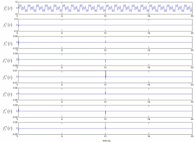
( ) ( ) 0 ln i i i WT j j j S p p p < ∑   = − ⋅ _ _ (2.28) where p is the time evolution of relative wavelet energy at a resolution level j in the time ( )ji

interval i ( ) ( ) ( ) i i j j i tol E p E = (2.29) These features were investigated by numerically simulated harmonic signals and two laboratory test cases. “It is demonstrate that wavelet-time entropy is a sensitive damage feature in detecting the abnormality in measured successive vibration signals; relative wavelet entropy is a good damage feature to detect damage occurrence and damage location through the vibration signals measured from the intact and damaged structures; and the relative wavelet entropy method is

(38)

flexible in choosing the reference signal simultaneously measured from any undamaged location of the target structure” (Ren and Sun 2008).

2.2 Pattern Recognition

Feature patterns represent different conditions of an analyzed structure or machine. The objective of pattern recognition in damage detection is to distinguish between different classes of patterns presenting these conditions based either on a prior knowledge or on statistical

information extracted from the patterns (Chang and Yang, 2004). Classical methods of pattern recognition use statistical and syntactic approaches. In recent years neural networks have been established as a powerful tool for pattern recognition. An overview of these methods can be found in Jain et al. (2000) and Duda et al. (2000). A brief description of some applications for damage detection is given below.

2.2.1 Fisher’s Discriminant

Fisher’s discriminant is a classification method that projects multi-dimensional feature vectors onto one-dimensional subspace to perform classification. The projection maximizes the distance between the mean of the two classes while minimizing the variance within each class. Farrar et al. (2001) defined Fisher’s discriminate using data from the vibration tests conducted on the columns under both undamaged condition and the damage condition of initial yielding of the steel reinforcement. “The time series were modeled using auto-regressive estimation referred to as linear predictive coding (LPC). Subsequent damage levels were then identified based on this same Fisher projection. When Fisher’s discriminant was applied to data from both sensors on undamaged and damaged columns, there was statistically separation between the LPC

coefficients for the undamaged cases and damaged cases. While increasing damage was not necessarily related to increasing Fisher coordinate, all damaged cases had a profile significantly different from that of the undamaged case”. The authors showed a strong potential for using linear discriminant operators to identify the presence of damage.

2.2.2 X-bar Control Chart

Sohn et al. (2000) applied a statistical process control (SPC) technique, known as an “X-bar control chart”, to monitoring a reinforced concrete bridge column. “Acceleration time series were recorded from the vibration tests of the bridge column and auto-regressive (AR) prediction

Structural damage detection using signal-based pattern recognition

Abstract

Copyright

Abstract

Table of Contents

List of Figures

List of Tables

Acknowledgements

Dedication

CHAPTER 1 - INTRODUCTION

1.1 Introduction

1.2 Objectives

CHAPTER 2 - LITERATURE REVIEW

2.1 Feature Extraction and Selection

2.1.1 Time-domain Methods

( )

( )

(

)

( )

∑

( )

( )

( )

( )

(

)

( )

( )

( )

( )

( )

( )

( )

( )

( )

( )

( )

[ ]

[ ]

[ ]

[ ]

[ ]

( )

( )

(

)

( )

(

)

(

)

( )

( )

( )

(

)

(

)

( )

( ) ( )

( )

( )

( )

{ }

{ }

( )

( )

( )

( )

2.1.2 Frequency-domain Methods

{

}

( )

( )

( )

( )

( )

( ) ( )

( ) (

_{( ) ( )}

_{( )}

_{( )}

_{( )}

_{( )}

_{( )}

_{( )}

_{( )}