Multivariate Rank Outlyingness and Correlation Effects

Volume 16 | Issue 1 Article 14

5-1-2017

Multivariate Rank Outlyingness and Correlation

Effects

Olusola Samuel Makinde

Department of Statistics, Federal University of Technology, P.M.B. 704, Akure, Nigeria, [email protected]

Follow this and additional works at:http://digitalcommons.wayne.edu/jmasm

Part of theApplied Statistics Commons,Social and Behavioral Sciences Commons, and the

Statistical Theory Commons

This Regular Article is brought to you for free and open access by the Open Access Journals at DigitalCommons@WayneState. It has been accepted for

Recommended Citation

Makinde, O. S. (2017). Multivariate rank outlyingness and correlation effects. Journal of Modern Applied Statistical Methods, 16(1), 246-260. doi: 10.22237/jmasm/1493597580

Olusola Samuel Makinde is a Lecturer in the Department of Statistics. Email at [email protected].

Multivariate Rank Outlyingness and

Correlation Effects

Olusola Samuel Makinde Federal University of Technology Akure, Nigeria

The effect of correlation on multivariate rank outlyingness, a result of deviation of multivariate rank functions from property of spherical symmetry, is examined. Possible affine invariant versions of this multivariate rank are surveyed, and outlyingness of affine invariant and non-invariant spatial rank functions under general affine transformation are compared.

Keywords: rank function, outlyingness function, symmetry, correlation

Introduction

Ordering of data and the search for the units lying far from the centroid is closely related to searching for outliers in the data cloud. In a univariate setting, this ordering is a linear ranking from smallest to largest. Given sample points

X1, X2, …, Xn, we can order them by their rank values. Ordering of univariate

objects based on rank does not depend heavily on the underlying distribution of the data, nor involve estimation of parameters of probability distributions. Similarly in a multivariate setting, we can order multivariate sample points

X1, X2, …, Xn by their rank function.

An appealing way of working with probability distributions in ℝd, especially

in nonparametric inference, is through “descriptive measures” that characterize features of particular interest (Serfling, 2004, p. 260). One attractive approach is to base the measures on outlyingness of multivariate rank. In the last couple of decades, notions of multivariate signs and ranks have become a useful tool in analyzing multivariate data, as it does not depend heavily on distributional assumptions, and characterizes the central and extreme observations quite

of data preserves the direction of the data. Möttönen & Oja (1995), Möttönen, Oja & Tienari (1997) used the notion of spatial ranks to construct multivariate tests of location.

A related notion to multivariate ranks is the data depth. Data depth measures

depth or centrality of a d-dimensional observation with respect to a multivariate

data cloud or underlying multivariate distribution. Depth functions in literature include Mahalanobis depth, half-space depth, simplicial depth, likelihood depth, and projection depth, among others. Liu, Parelius & Singh (1999) proposed various ideas on analyzing multivariate data using data depths. We refer readers to Liu, Parelius & Singh (1999) for detailed discussion on depth functions. Statistical approaches based on most of these depth functions suffer computational complexities of the depth functions.

The spatial rank and its outlyingness can be applied in classification and

clustering (Makinde, 2015). It has been applied in construction of geometric

quantile (Chaudhuri, 1996; Serfling, 2004). It is well known that multivariate rank

is not invariant under arbitrary affine transformations, so it may be affected by deviation of population distribution from spherical symmetry. Effect of this deviation on spatial rank outlyingness will be investigated. Based on this, we shall introduce a way of constructing affine invariant multivariate rank outlyingness.

Spatial Rank

Signs and ranks are commonly used in statistical methodology to develop methods or procedures that are independent of distribution assumptions. Use of rank for computing statistical quantities gives robust estimators (e.g. estimator for location) as they are not affected by the presence of outlying values in the data. For the univariate data, sign of x ℝ can be defined as

 

1, 0 0, 0 1, 0 x sign x x x     _   _  or equivalently,

 

, 0 0, 0 x x x sign x x  _     _ 

Univariate centred rank of x with respect to data points X1, X2, …, Xn from

distribution F can be defined as

 





1 1 . n i i rank x sign x X n  





Following are some of the basic properties of rank(x),

1. | rank(x) | ≤ 1.

2. | rank(x) | = 0 implies x is the median and | rank(x) | = 1 implies x is an extreme point.

3. E(| rank(x) |) = 2F(x) – 1

These properties suggest that rank(x) is not only a useful descriptive statistics, it also characterizes the distribution. Now, we want to define sign and rank functions in a multivariate set up following Chakraborty (2001). Suppose

x ℝd, then the lp sign of x is

 

 

1, , p p p p sign           _  0 0 0 x x x x x x x where





 



 

 



1 1 2 1 1 1 1 and , , . p p p p d p p p d d x x x sign x x sign x x



       x x

The lp rank of x  ℝd with respect to data points X1, X2, …, Xn  ℝd is

defined as

 





1 1 . n p p i i rank sign n  



 x x X

when p = 1, sign

 

x 



sign x

 

₁ ,sign x

 

₂ , ,sign x

 

_d



T, the vector of co-ordinatewise signs and for p = 2,

 

2

2

sign x  x

x

where ||.||2 is the Euclidean norm defined as





1 2 2 2 2 1 2 2  y y  yd . y

sign2(x)is called the spatial sign vector.

Suppose X is a d-dimensional random vector having a distribution F, which

is assumed to be absolutely continuous with respect to the Lebesgue measure ℝd.

The spatial rank function (Möttönen & Oja, 1995) of any point x  ℝd with respect to F is defined as

 

. F F rank E _  _    x X x x X (1)

Here ||.|| is the usual Euclidean norm. It follows immediately from the definition that rankF(x) = 0 implies that x is the spatial median of the multivariate

distribution F. Koltchinskii (1997) established that this spatial rank function is a one-to-one function of the distribution function F and hence it characterizes the distribution. Moreover the direction of the vector rankF(x) suggests the direction

in which x is extreme compared to the distribution. Using this idea, Serfling (2004) introduced ||rankF(x)|| as a measure of outlyingness and defined several

descriptive measures. Smaller values of ||rankF(x)|| implies that x is more central

to the distribution and larger values of ||rankF(x)|| indicates that x is more extreme.

If ||rankF(x)|| = 0, then x is the spatial median.

Spatial rank helps determine the geometric position of points in ℝd with

respect to the data cloud, and hence can be viewed as a descriptive statistic (Guha,

2012). Suppose F is spherically symmetric and characterized by location

parameter θ ℝd, ||rankF(x)|| increases as ||x − θ|| increases. This result is stated

formally in Theorem 1 below:

Theorem 1. If x has spherically symmetric distribution F with θ as the

 





F rank q







    x x x x

for some increasing, non-negative function q.

This is proved in Guha (2012). Following Theorem 1, smaller rank

outlyingness indicates more central observation and larger rank outlyingness indicates extreme observation. The following results hold for rank outlyingness:

Fact: Let ||rankF(x)|| denote the measure of outlyingness of rankF(x).

Then

1. ||rankF(x + θ)|| = ||rankF(x)|| for a constant vector θ.

2. ||rankF(Ax)|| = ||rankF(x)|| for an orthogonal matrix A.

The first expression above implies that rank outlyingness is invariant under location shift or translation while the second indicates that rank outlyingness is invariant under orthogonal scale transformation. In practice, the rank functions

rankF will hardly be known completely and we need to estimate them from the

training sample. Let X1, X2, …, Xn ℝd be a random sample from a population

having distribution F. We define the empirical rank function as

 

1 1 n n i F i i rank n    



x X x x X

Theorem 2. Let X1, X2, …, Xn be independent and identically

distributed d-dimensional random vectors having distribution function F, which is

absolutely continuous, then as n ,

 

 

sup 0. n d F F rank rank    x x x

The proof follows from Koltchinskii’s (1997) work on the convergence of the empirical version of spatial rank to its population analogue.

Chaudhuri (1996) defined spatial quantiles as vectors in d that are indexed



| , 1 .



d d

B  u u u  For any

u



d and

t



d , also define

 

, , ,

 u t  t  u t where .,. denotes the usual Euclidean inner product.

Spatial quantile corresponding to u and based on X1, X2, …, Xn  d is defined as

 





1 ˆ _{arg min , .} d n n i Q i Q Q  _ 



  u u X

It follows from Theorem 1.1.2 of Chaudhuri (1996) that

 

 

1 0 n n i i n i Q n Q     



u X u u X

if Qn(u) ≠ Xi for all 1 ≤ i ≤ n. This implies

 

 

1 1 n n i i n i Q n  Q  



u X u = u X . (2) Serfling (2004) defined

 

n F

rank x as the inverse function of the spatial

quantile function, Q uˆ_n

 

. Mathematically, we can write (2) as

 



ˆ



 

n n F n F rank Q rank  

u u x and so Qˆn

 

u  x implies rankF_n

 

x u. It

follows that

 

n

F

rank x is the inverse function of the multivariate geometric

quantile function Qn(u) in the sense that rankF_n

 

x u implies that Qn(u) = x and vice-versa.

Effect of correlation on rank outlyingness

The distribution of a random variable X is said to be spherically symmetric about

a parameter θ if, for any orthogonal matrix B,





d



 

X  B X 

The density function of any spherically symmetric distribution of a random variable X, if it exists, is of the form f

 

x g





x

 

T x





for some

nonnegative scalar function g(.). Similarly, the distribution of a random vector X

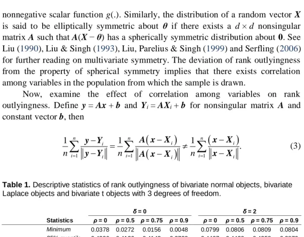
is said to be elliptically symmetric about θ if there exists a d × d nonsingular matrix A such that A(X − θ) has a spherically symmetric distribution about 0. See Liu (1990), Liu & Singh (1993), Liu, Parelius & Singh (1999) and Serfling (2006) for further reading on multivariate symmetry. The deviation of rank outlyingness from the property of spherical symmetry implies that there exists correlation among variables in the population from which the sample is drawn.

Now, examine the effect of correlation among variables on rank outlyingness. Define y = Ax + b and Yi = AXi + b for nonsingular matrix A and

constant vector b, then













1 1 1 1 1 1 . n n n i i i i i i i i i n  n  n         



y Y



A x X



x X y Y A x X x X (3)

Table 1. Descriptive statistics of rank outlyingness of bivariate normal objects, bivariate Laplace objects and bivariate t objects with 3 degrees of freedom.

δ = 0 δ = 2 Statistics ρ = 0 ρ = 0.5 ρ = 0.75 ρ = 0.9 ρ = 0 ρ = 0.5 ρ = 0.75 ρ = 0.9 Bivariate normal distribution Minimum 0.0378 0.0272 0.0156 0.0048 0.0799 0.0806 0.0809 0.0804 25% quantile 0.4396 0.4136 0.4143 0.3739 0.4497 0.4430 0.4258 0.3870 Median 0.6263 0.6405 0.6157 0.5794 0.6069 0.5900 0.5774 0.5503 Mean 0.6021 0.5986 0.5873 0.5693 0.6053 0.6007 0.5900 0.5711 75% quantile 0.7827 0.7852 0.7767 0.7665 0.7948 0.7724 0.7408 0.7524 Maximum 0.9647 0.9649 0.9846 0.9941 0.9637 0.9678 0.9714 0.9900 Bivariate Laplace distribution Minimum 0.0687 0.0673 0.0589 0.0607 0.0459 0.0588 0.0655 0.0732 25% quantile 0.4346 0.4429 0.4114 0.3797 0.3688 0.3693 0.3749 0.3770 Median 0.6133 0.6076 0.5717 0.5410 0.6244 0.6089 0.5749 0.5691 Mean 0.5952 0.5894 0.5791 0.5649 0.5934 0.5868 0.5762 0.5618 75% quantile 0.7611 0.7646 0.7821 0.7742 0.7986 0.7942 0.7853 0.7664 Maximum 0.9693 0.9763 0.9800 0.9832 0.9819 0.9925 0.9955 0.9976 Bivariate t distribution with 3 d.f. Minimum 0.1054 0.1129 0.1050 0.0871 0.0883 0.0865 0.0899 0.0698 25% quantile 0.4076 0.4075 0.3900 0.3569 0.4260 0.4158 0.4098 0.3951 Median 0.6188 0.5967 0.5705 0.5433 0.6054 0.6009 0.5817 0.5566 Mean 0.5940 0.5849 0.5716 0.5546 0.5945 0.5885 0.5783 0.5630 75% quantile 0.8034 0.7875 0.7682 0.7656 0.7734 0.7715 0.7890 0.7600 Maximum 0.9833 0.9843 0.9927 0.9978 0.9948 0.9964 0.9986 0.9996

As illustration of the effect of correlation on rank outlyingness in (3), a small simulation study is presented. Consider a population to be bivariate elliptically symmetric with centre of symmetry μ = (δ 0)T _{and scale matrix}

1 1





     

 . Simulate a random sample X1, X2, …, Xn, where sample size n is taken to be 100, and estimate the rank outlyingness function. For various values of ρ, Table 1 presents rank outlyingness for bivariate normally distributed sample, bivariate Laplace distributed sample and bivariate t distributed sample with 3 degrees of freedom.

The outlyingness function behaves anomalously for different values of



0,1



 irrespective of class distribution. For each family of distribution,

descriptive statistics are not in any specific order of ρ. The reason is that though the distribution of Xi is taking more ellipsoid form as ρ increases, the rank

outlyingness is being computed with respect to sphere as spatial rank is invariant under affine transformation. To overcome the problem of affine non-invariance property of spatial rank, affine invariant versions of rank outlyingness are suggested next.

Affine Invariant Rank Function

Approach based on Cholesky decomposition of the covariance matrix

Spatial rank function can also be defined (Makinde & Chakraborty, 2015) as

 

1



_



_

* 1 F F rank E    _      _    V x X x V x X

where V is a d × d matrix such that VVT = cΣ for some constant c. If the

covariance of the distribution F exists, we can take V to be the Cholesky

decomposition of the covariance matrix. For the empirical versions, one can

estimate Σ by minimum covariance determinant (MCD) estimator of Rousseeuw

(1984) and then V by its square root matrix. Note that, the Choleski

decomposition of Σ (or, its estimate) may not produce an affine invariant rank

function but the outlyingness function rank_F*

 

x will be affine invariant

Transformation and re-transformation approach

Chakraborty & Chaudhuri (1996) proposed transformation and re-transformation

methodology for conversion of non-equivariant and non-invariant measures under affine transformation to affine equivariant and affine invariant versions respectively, using data driven coordinate system. and then used to construct an affine equivariant median. This technique was also used in Chakraborty &

Chaudhuri (1998) to construct robust estimate of location; in Chakraborty,

Chaudhuri & Oja (1998) to construct an affine equivariant median and angle test;

in Chakraborty (2001) to construct an affine equivariant quantile and also in Dutta

& Ghosh (2012); and in Makinde & Chakraborty (2015) to construct affine invariant classifier. The concept is to form an appropriate data driven coordinate system and express all the data points in terms of the new coordinate system. Then compute the spatial rank of the transformed data. Define







| 1, 2, , and 1



n

S    n   d

as the collection of all d + 1 subset of {1, 2, ..., n}. For a fixed

α = {i0, i1, …, id}



Sn, we define X(α) to be a d × d matrix whose columns are 1 0, 2 0, , d 0.

i i i i i i

X X X X X X That is, one of the d + 1 data points determines

the origin and the lines joining that origin to the remaining d data point will form

the coordinate system.

Assuming that elements of α are naturally ordered and that Xi's are

independent and identically distributed observations with common probability distribution, which is absolutely continuous with respect to the Lebesgue measure in d, X(α) is invertible with probability one (Chakraborty, 2001). So, X(α) is the

transformation matrix and for each i



, the data set Xi is transformed into a new

coordinate system, Yi = {X(α)}−1Xi and then compute the rank of y = {X(α)}−1x.

X(α) is chosen in such a way that the columns of 12_X

 

 _{are as orthogonal as}

possible. Because population covariance matrix Σ is unknown in practice,

compute its estimate from the data. The choice of α depends on the value of α that

minimizes

 





 



 



 





 





1 1/ 1 / det T d T trace   d          X X X X

so that ζ(α) becomes very close to 1. Obviously, once α is selected, the computation of affine invariant spatial rank is straightforward in any dimension.

The affine invariant spatial rank is defined as

 



 







 









1 1 F rank E      _      _      X x X x X x X (4)

The sample version is defined as

 



 







 









1 1 1 1 n n i F i i rank n





     



X x X x X x X (5)

Suppose Xi, 1 ≤ i ≤ n be samples on d from a distribution F, it is easy to

show that the rank function (defined in (5) above) of a data point y = Ax + b is

rankG(y) = rankF(x), where G is the distribution of y. This is shown by the

theorem below.

Theorem 3. Suppose Xi, 1 ≤ i ≤ n is a sample on d having a

distribution F. For any



S_n,

 

n

F

rank x defined in (5) is affine invariant.

Hence, the transformed multivariate rank is invariant under affine transformation. Any statistic based on this transformed rank is affine invariant and can handle the problem associated with deviation from spherical symmetry. Gao

(2003) defined another version of spatial depth based on rank outlyingness

defined in (1) and can be made affine invariant by replacing outlyingness of the rank function in (1) by its affine invariant version.

Numerical Example

To illustrate these methodologies, an example based on ordering of iris data (Fisher, 1936) is presented and quantiles of outlyingness functions of the variants of multivariate rank for the three species of iris flower are compared. The species are iris setosa, iris versicolor and iris virginica.

Presented in Table 2 are the quantiles and mean of the outlyingness of affine invariant and non-affine invariant rank for three species of iris data. The data is available on package R. We denote outlyingness function of affine invariant multivariate rank based on Cholesky decomposition of the covariance matrix by CD approach, outlyingness function of affine invariant multivariate rank based on transformation and re-transformation approach by TR approach and outlyingness

function of affine non-invariant multivariate rank defined in equation (1) by

non-invariant.

Observe that quantiles of rank outlyingness based on Cholesky decomposition of the covariance matrix and one based on transformation and re-transformation approach are close to each but far away from corresponding quantiles of values of outlyingness based on affine non-invariant multivariate rank. The implication of this is that correlation among the four variables (sepal length, sepal width, petal length and petal width) of each observation in the data can affect the performance of any statistical method or test based on non-affine invariant rank outlyingness.

Table 2. Ordering of species of Iris data based on the outlyingness functions of affine invariant and non-affine invariant ranks.

Iris Species Approaches Minimum 1st Quartile Median Mean 3rd Quartile Maximum Setosa CD approach 0.2461 0.5500 0.6805 0.6447 0.7740 0.8827 TR approach 0.2456 0.5383 0.6792 0.6437 0.7791 0.8820 Non-invariant 0.1398 0.5138 0.6372 0.6160 0.7640 0.9436 Versicolor CD approach 0.2727 0.5520 0.6811 0.6506 0.7682 0.8755 TR approach 0.2710 0.5532 0.6862 0.6485 0.7603 0.8676 Non-invariant 0.2992 0.4759 0.6406 0.6197 0.7317 0.9116 Virginica CD approach 0.3879 0.5578 0.6724 0.6543 0.7382 0.8877 TR approach 0.3513 0.5394 0.6722 0.6531 0.7596 0.9063 Non-invariant 0.2808 0.4850 0.6447 0.6204 0.7439 0.9538

Observe that range of outlyingness of observations is noticeably bigger in affine non-invariant rank compare to the affine invariant rank. The minimum outlyingness value is least in affine non-invariant rank and may therefore mis-identify an observation as outlying. Hence, both affine invariant rank outlyingness functions perform quite well.

Conclusion

The effect of correlation on spatial rank outlyingness was considered and its possible applications. The spatial rank outlyingness based on the training sample does not depend on any distributional assumption and does not require any estimation of model parameters. These give a nonparametric flavor to any statistical technique based on multivariate rank. It is also computationally simple and can be applied to very high dimensional data as well. The rank outlyingness is not affine invariant and as a remedial measure we suggested a transformation of the data to a new coordinate system to make the rank outlyingness affine invariant.

The first idea of transformation is based on transformation retransformation

approach proposed by Chakraborty (2001). This makes the spatial ranks affine

invariant and hence the rank outlyingness becomes affine invariant. The other transformation considered is based on the square root of the scale matrix Σ. It requires the estimation of Σ and may result in a non-robust rank outlyingness. Though the resulting spatial ranks are not affine invariant, rank outlyingness is affine invariant and usually computationally very simple if we use the sample

covariance matrix as an estimate of Σ. When variables of the data are independent

of one another, then both affine invariant versions of rank outlyingness reduces to the usual rank outlyingness.

References

Chakraborty, B. (2001). On affine equivariant multivariate quantiles. Annals

of the Institute of Statistical Mathematics, 53(2), 380–403. doi:

10.1023/a:1012478908041

Chakraborty, B. & Chaudhuri, P. (1996). On a transformation and retransformation technique for constructing affine equivariant multivariate

median. Proceedings of the American Mathematical Society, 124(8), 2539–2546.

doi: 10.1090/s0002-9939-96-03657-x

Chakraborty, B. & Chaudhuri, P. (1998). On an adaptive transformation and

retransformation estimate of multivariate location. Journal of the Royal Statistical

Society: Series B, 60(1), 145–157. doi: 10.1111/1467-9868.00114

Chakraborty B., Chaudhuri, P. & Oja, H. (1998). Operating transformation

and re-transformation on spatial median and angle test. Statistica Sinica, 8, 767–

Chaudhuri, P. (1996). On a geometric notion of quantiles for multivariate

data. Journal of American Statistical Association, 91(434), 862–872. doi:

10.1080/01621459.1996.10476954

Dutta, S. & Ghosh, A. K. (2012). On classification based on Lp depth with an adaptive choice of p. Technical Report No. R5/2011, Statistics and

Mathematics Unit. Indian Statistical Institute, Kolkata, India

Fisher, R. A. (1936). The use of multiple measurements in taxonomic

problems. Annals of Eugenics, 7(2), 179–188. doi:

10.1111/j.1469-1809.1936.tb02137.x

Gao, Y. (2003). Data depth based on spatial rank. Statistics & Probability Letters, 65(3), 217 – 225. doi: 10.1016/j.spl.2003.06.003

Guha, P. (2012). On scale-scale curves for multivariate data based on rank

regions. PhD thesis, University of Birmingham, UK.

Koltchinskii, V. I. (1997). M-estimation, convexity and quantiles. The

Annals of Statistics, 25(2), 435 – 477. doi: 10.1214/aos/1031833659

Liu, R. Y. (1990). On a notion of data depth based on random simplices. The

Annals of Statistics, 18(1), 405–414. doi: 10.1214/aos/1176347507

Liu, R. Y. & Singh, K. (1993). A quality index based on multivariate data

depth and multivariate rank tests. Journal of the American Statistical Association,

88(421), 252–260. doi: 10.1080/01621459.1993.10594317

Liu, R. Y., Parelius, J. M. & Singh, K. (1999). Multivariate analysis by data

depth: Descriptive statistics, graphics and inference. The Annals of Statistics,

27(3), 783–858. doi: 10.1214/aos/1018031260

Makinde, O. S. (2015). On some classification methods for high

dimensional and functional data. PhD Thesis, University of Birmingham Makinde, O. S. & Chakraborty, B. (2015). On some classifiers based on distribution functions of multivariate ranks. In Nordhausen, K and Taskinen, S.

(Eds). Modern Nonparametric, Robust and Multivariate Methods, Festschrift in

Honour of Hannu Oja. NY: Springer, 249–264. doi: 10.1007/978-3-319-22404-6_15

Möttönen, J. & Oja, H. (1995). Multivariate spatial sign and rank methods.

Journal of Nonparametric Statistics, 5, 201–213.

Möttönen, J., Oja, H. & Tienari, J. (1997). On the efficiency of multivariate spatial sign and rank tests. The Annals of Statistics, 25(2), 542–552. doi:

Rousseeuw, P. J. (1984). Least median of squares regression. Journal of the American Statistical Association, 79(388), 871–880. doi:

10.1080/01621459.1984.10477105

Serfling, R. (2004). Nonparametric multivariate descriptive measures based

on spatial quantiles. Journal of Statistical Planning and Inference, 123(2), 259–

278. doi: 10.1016/s0378-3758(03)00156-3

Serfling, R. (2006). Multivariate symmetry and asymmetry, In S. Kotz, N.

Balakrishnan, C. B. Read & B. Vidakovic, Eds. Encyclopedia of Statistical

Sciences, Second Ed., 8, 5338–5345. NY: Wiley. doi:

10.1002/0471667196.ess5011.pub2

Appendix

Proof of Theorem 3. For any d × d nonsingular matrix A, let Yi = AXi + b.

Since X(α)=[Xi1 − Xi0, Xi2 − Xi0, ..., Xid− Xi0], we have

 

























 

1 0 2 0 0 1 0 2 0 0 1 0 2 0 0 1 0 2 0 0 , , , , , , , , , , , , i i i i id i i i i i id i i i i i id i i i i i id i       _          _          Y Y Y Y Y Y Y AX b AX b AX b AX b AX b AX b AX AX AX AX AX AX A X X X X X X AX

The transformed multivariate rank of a data point y = Ax + b, where

x



d

 





 









 









 









 









 









 









 









 









 

1 1 1 1 1 1 1 ₁ 1 ₁ 1 1 1 1 1 1 1 1 . n n n G G n i i i n i i i n i i _i n i F i i rank rank n n n rank n                _  _                               









y AX b Y y Y Y y Y AX Ax b AX b AX Ax b AX b X A A x X X A A x X X x X x X x X