THESIS FOR THE DEGREE OF DOCTOR OF PHILOSOPHY
Machine Learning Methods Using Class-specific
Subspace Kernel Representations
for Large-Scale Applications
Yinan Yu
Department of Signals and Systems
CHALMERS UNIVERSITY OF TECHNOLOGY Göteborg, Sweden 2016
for Large-Scale Applications Yinan Yu
ISBN 978-91-7597-487-3 c
Yinan Yu, 2016.
Doktorsavhandlingar vid Chalmers tekniska högskola Ny serie nr 4168
ISSN 0346-718X
Department of Signals and Systems Chalmers University of Technology SE–412 96 Göteborg
Sweden
Telephone + 46 (0)31 – 772 1000
Typeset by the author using LATEX.
Chalmers Reproservice Göteborg, Sweden 2016
Abstract
Kernel techniques became popular due to and along with the rising success of Support Vector Machines (SVM). During the last two decades, the kernel idea itself has been extracted from SVM and is now widely studied as an independent subject. Essentially, kernel methods are nonlinear transformation techniques that take data from an input set to a high (possibly infinite) dimensional vector space, called the Reproducing Kernel Hilbert Space (RKHS), in which linear models can be applied. The original input set could be data from different domains and applications, such as tweets, ratings of movies, images, medical measurements, etc. The two spaces are connected by a Positive-Semi Definite (PSD)kernel function and all computations in the RKHS are evaluated on the low dimensional input set using the kernel function.
Kernel methods are proven to be efficient on various applications. However, the computational complexity of most kernel algorithms typically grows cubically, or at least quadratically, with respect to the training size. This is due to the fact that a Gram kernel matrix needs to be constructed and/or inverted. To improve the scalability for large-scale training, kernel approximation techniques are employed, where the kernel matrix is assumed to have a low-rank structure. Essentially, this is equivalent to assuming a subspace model spanned by a subset of the training data in the RKHS. The task is hence to estimate the subspace with respect to some criteria, such as the reconstruction error, the discriminative power for classification tasks, etc. Based on these motivations, this thesis focuses on the development of scalable kernel techniques for supervised classification problems. Inspired by the idea of the subspace classifier and kernel clustering models, we have proposed the CLAss-specific Subspace Kernel (CLASK) representation, where class-specific kernel functions are applied and individual subspaces can be constructed accordingly. In this thesis work, an automatic model selection technique is proposed to choose the best multiple kernel functions for each class based on a criterion using the subspace projection distance. Moreover, subset selection and transformation techniques using CLASK are developed to further reduce the model complexity with an enhanced discriminative power for kernel approximation and classification. Furthermore, we have also proposed both a parallel and a sequential framework to tackle large-scale learning problems.
Acknowledgement
I would like to take this opportunity to thank Prof. Mats Viberg and Prof. Tomas McKelvey for giving me the opportunity to join the Signal Processing group as a PhD candidate. I have been very happy studying and working here.
My deepest gratitude goes to my advisor Prof. Tomas McKelvey. We started the tradition of our one hour-ish weekly meetings when I did my master thesis project on radar signal processing, and it has been a long journey since then. I really appreciate all the technical discussions we had all these years and enjoyed every trip we took together. You have helped me through so many tough moments with full supports and great patience. Nothing would have been possible without you. I would also like to thank my (almost) co-advisor Prof. Konstantinos Diamantaras. I cherish all the discussions and fun we had, not to mention the wonderful visit in Thessaloniki. I am always impressed by all your awesome research ideas and your ability in finding crazy photo opportunities. I would like to express many many thanks to Prof. S.Y. Kung for being a great advisor and delightful host at Princeton. You always challenge me and give me genius advice. Thanks for including me in the wrapping up of your book writing process. The book is exceptional and I have learned so much from you.
I would like to thank Prof. Jian Yang at Chalmers, who was also my advisor during my master thesis project. You have helped me so much both professionally and personally. Without you, it would not have been the same.
Many thanks to my co-authors and colleagues from Medfield Diagnostics AB and Chalmers University of Technology. Hana Dobsicek Trefna, I really enjoyed working and chatting with you and I will see you soon as we still have some future work to do together (those rotten wood logs ain’t gonna detect themselves). I would like to thank Prof. Mikael Persson. Thanks for including me in those interesting and promising projects, such as the Stroke Finder. It has been very nice working with you and you are such a delightful person. Many thanks to my co-authors Andreas Fhager and Stefan Candefjord for the nice collaboration. Also thank you Stefan Kidborg. I have not seen you for a long time, but all the work we have done together is memorable. I still kept the candy basket you gave me (only the basket - the candies are gone). Thank you Ann-Christine Lindbom, Natasha Adler Grønbech, Agneta Kinnander and Madeleine Persson for your efficient replies and assistances all these years.
This work has in part been funded by the Swedish Research Council (Vetenskap-srådet) under the contract number A0462701 which is gratefully acknowledged.
Yinan Yu Göteborg, 2016
List of Included Publications
PAPER 1
Y. Yu, T. McKelvey and S.Y. Kung, “Kernel SODA: a feature reduction tech-nique using kernel based analysis”, In Proceedings of the 12th International Conference on Machine Learning and Applications (ICMLA), pages 72-78, Mi-ami, FL, USA, 2013.
PAPER 2
Y. Yu and T. McKelvey, “Learning hierarchical feature space using CLAss-specific Subspace Multiple Kernel - Metric Learning for classification”,submitted to Journal of Machine Learning Research (JMLR).
PAPER 3
Y. Yu, T. McKelvey, K.I. Diamantaras and S.Y. Kung, “Enhanced distance subset approximation using class-specific kernel functions for supervised learn-ing”, submitted to Neural Networks and Learning Systems, IEEE Transaction on.
PAPER 4
Y. Yu and T. McKelvey, “Kernel subspace empirical intersection removal for kernel approximation and classification”, submitted to Neural Networks and Learning Systems, IEEE Transaction on.
PAPER 5
Y. Yu, T. McKelvey, K.I. Diamantaras and S.Y. Kung, “CLAss-specific Sub-space Kernel representations and adaptive margin slack minimization for large scale classification”, accepted for publication in Neural Networks and Learning Systems, IEEE Transaction on.
Software Package
https://github.com/yinan16/DeepCLASK
Other Publications
• Y. Yu, K. I. Diamantaras, T. Mckelvey and S.Y. Kung, “Enhanced distance subset approximation using class-specific subspace kernel representation for ker-nel approximation”,In Proceeding of IEEE International Workshop on Machine Learning for Signal Processing, Vietri sul Mare, Salerno, Italy, 2016.
• Y. Yu, K. I. Diamantaras, T. McKelvey and S.Y. Kung, “Adaptive margin slack minimization in RKHS for classification”,In Proceedings of the 38th IEEE
• Y. Yu, and T. McKelvey, “A robust subspace classification scheme based on empirical intersection removal and sparse approximation”,Integrated Computer-Aided Engineering, 22 (1), pages 59-69, 2015.
• Y. Yu, T. McKelvey, and S.Y. Kung, “Feature reduction based on Sum-of-SNR (SOSum-of-SNR) optimization”, In Proceedings of the 39th IEEE International Conference on Acoustics, Speech, and Signal Processing (ICASSP), pages 6756-6760, 2014.
• Y. Yu, K. I. Diamantaras, T. McKelvey and S.Y. Kung, “Multiclass Ridge-adjusted Slack Variable Optimization Using selected basis for fast classification”,
In Proceedings of the 22nd European Signal Processing Conference (EUSIPCO), pages 1178-1182, Lisbon, Portugal, 2014.
• Y. Yu, “Classification of high dimensional signals with small training sample size with applications towards microwave based detection systems”, Licentiate Thesis, Chalmers University of Technology, 2013.
• Y. Yu, T. McKelvey and S.Y. Kung, “A classification scheme for ’high-dimensional-small-sample-size’ data using SODA and ridge-SVM with microwave measure-ment applications”, In Proceedings of the 38th IEEE International Conference on Acoustics, Speech and Signal Processing (ICASSP), Vancouver, Canada, 2013.
• Y. Yuand T. McKelvey, ”A unified subspace classification framework developed for diagnostic system using microwave signal”, In Proceedings of the 21st Euro-pean Signal Processing Conference (EUSIPCO), Marrakech, Morocco, 2013. • Y. Yu, K. I. Diamantaras, T. McKelvey and S.Y. Kung, “Ridge-Adjusted Slack
Variable Optimization for supervised classification”,In Proceedings of IEEE In-ternational Workshop on Machine Learning for Signal Processing, Southamp-ton, United Kingdom, 2013.
• Y. Yu and T. McKelvey, “A subspace learning algorithm for microwave scat-tering signal classification with application to wood quality assessment”, In Proceeding of IEEE International Workshop on Machine Learning for Signal Processing, Santander, Spain, 2012.
• Y. Yu, J. Yang and T. McKelvey “Compact UWB indoor and through-wall radar with precise ranging and tracking”, International Journal of Antennas and Propagation, 2012. 2011
• Y. Yu, S. Maalik, J. Yang, T. McKelvey, K. Malmström, L. Landen and B. Stoew, “A new UWB radar system using UWB CMOS chip”, In Proceedings of
the 5th European Conference on Antennas and Propagation (EUCAP), Rome, Italy, 2011.
• M. Persson, A. Fhager, H. D. Trefna, Y. Yu, T. McKelvey, G. Pegenius, J-E Karlsson and Mikael Elam, “Microwave-based stroke diagnosis making global prehospital thrombolytic treatment possible”, IEEE Transactions on Biomedi-cal Engineering 61 (11), pages 2806-2817, 2014.
• Q. Jian, J. Yang,Y. Yu, P. Bjorkholmy and T. McKelvey, “Detection of breath-ing and heartbeat by usbreath-ing a simple UWB radar system”, In Proceedings of the 8th European Conference on Antennas and Propagation (EuCAP), pages 3078-3081, The Hague, The Netherlands, 2014.
• S. Candefjord, J. Winges, Y. Yu, T. Rylander and T. McKelvey, “Microwave technology for localization of traumatic intracranial bleedings - a numerical simulation study”, In Proceedings of the 35th Annual International Conference of the IEEE Engineering in Medicine and Biology Society (EMBC), pages 1948-1951, Osaka, Japan, 2013.
• R. Rothe, Y. Yu, and S.Y. Kung, “Parameter design tradeoff between pre-diction performance and training time for ridge-SVM”, In Proceeding of IEEE International Workshop on Machine Learning for Signal Processing, pages 1-6, Southampton, United Kingdom, 2013.
Contents
Contents ix
I
Introductory Chapters
1 Introduction 1
1.1 A Machine that Learns . . . 1
1.2 Learning Process . . . 2
1.3 Kernel Techniques . . . 3
1.4 Challenges . . . 6
1.4.1 Bias and Variance . . . 6
1.4.2 Robustness . . . 7
1.4.3 Scalability . . . 8
1.4.4 Hyperparameter Tuning . . . 8
1.5 Conclusion . . . 9
2 Reproducing Kernel Hilbert Space and its Application 11 2.1 Brief Review on Functional Analysis . . . 12
2.1.1 Hilbert Space . . . 12
2.1.2 Riesz Representation Theorem . . . 16
2.2 Reproducing Kernel Hilbert Space (RKHS) and Feature Maps . . . . 17
2.2.1 Reproducing Kernels . . . 17
2.2.2 Kernel Functions . . . 18
2.2.3 Constructing Feature Maps from Kernel Functions . . . 21
2.2.4 Dimension of the Feature Space . . . 22
2.3 Structural Risk Minimization and the Representer Theorem . . . 24
2.3.1 Convergence in RKHS . . . 24
2.3.2 Statistical Learning Theory and Structural Risk Minimization 25 2.3.3 Representer Theorem . . . 28
2.3.4 Kernel Tricks . . . 29
2.4 Conclusion . . . 30
3 Kernel Methods in Practice 33 3.1 Notations . . . 34
3.2.1 Cross-Validation . . . 36
3.2.2 Multiple-Kernel (MK) Model . . . 36
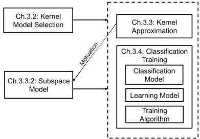
3.3 Kernel Approximation . . . 37
3.3.1 Motivation . . . 37
3.3.2 Subspace Model for Kernel Approximation . . . 38
3.3.3 Subspace Estimation . . . 40
3.4 Classification Training . . . 41
3.4.1 Overview . . . 41
3.4.2 Connection to Kernel Approximation: . . . 43
3.4.3 Example: LS-SVM . . . 45
3.5 Conclusion . . . 49
4 Summary of Included Papers 51 4.1 Kernel Subspace Model . . . 53
4.1.1 Overview . . . 53
4.1.2 Included Papers . . . 53
4.2 CLAss-specific Subspace Kernel (CLASK) Function for Classification 53 4.2.1 Class-specific Subspace Model . . . 53
4.2.2 CLAss-Specific Kernel (CLASK) Function . . . 54
4.2.3 Feature Map . . . 55
4.2.4 Included Papers . . . 55
4.2.5 A Feature Transformation System Using CLASK . . . 57
4.3 Software Package: DeepCLASK . . . 59
4.4 Conclusions . . . 59
5 Future work 61 References 63
II
Included Papers
Paper 1 Kernel SODA: A Feature Reduction Technique Using Kernel Based Analysis 73 1 Introduction . . . 732 Related Work . . . 74
2.1 Linear Discriminant Analysis (LDA) . . . 74
2.2 Principal Component Analysis (PCA) . . . 74
2.3 Successively Orthogonal Discriminant Analysis . . . 75
3 Theory of kernel SODA . . . 77
3.1 KSODA in Intrinsic Space . . . 77
3.2 KSODA in Empirical Space . . . 78
4 Implementation and approximation . . . 79
4.1 KSODA implementation . . . 79
CONTENTS
4.3 Data selection and numerical invertibility . . . 80
5 Experimental Results . . . 81
6 Acknowledgment . . . 83
References 87 Paper 2 Learning Hierarchical Feature Space Using CLAss-specific Subspace Multiple Kernel - Metric Learning for Classification 91 1 Introduction . . . 91
2 Problem formulation . . . 94
2.1 Distance metric and subspace model for a given kernel function 94 2.2 CLAss-specific Subspace Kernel Functions . . . 99
2.3 The CLAss-Specific Multiple-Kernel model . . . 101
3 Algorithms and implementation . . . 102
3.1 Basis matrix Uc,k . . . 102
3.2 Kernel function kc . . . 103
3.3 Summary of the Algorithm . . . 104
3.4 Remarks . . . 104
4 Learning Hierarchical CLASMK Feature Network . . . 105
5 Experimental Results . . . 107
5.1 One Layer CLASK-ML and CLASMK-ML Compared to Single Kernel Learning . . . 109
5.2 Multi-Layer CLASMK-ML Compared to Other Multi-Layer MK Techniques . . . 111
5.3 Multi-Layer CLASMK-ML Performance with Respect to the Number of Layers . . . 112
5.4 Visual Examples of the Estimated Weights . . . 113
6 Conclusion . . . 114 7 Appendix . . . 128 7.1 Lemma 2.2 . . . 128 7.2 Lemma 2.3 . . . 128 7.3 Proof of Theorem 2.2 . . . 129 References 131 Paper 3 Enhanced Distance Subset Approximation using Class-specific Kernel Functions for Supervised Learning 135 1 Introduction . . . 135
2 Class-specific Kernel Subspace Representation . . . 137
2.1 Notations . . . 137
2.2 Low Rank Approximation . . . 137
2.3 Relation to Subspace Model . . . 138
2.5 CLAss-Specific Kernel (CLASK) function: Feature Space and
Low Rank Approximation . . . 139
3 CLASK Parameter Estimation for Classification . . . 142
4 Algorithm . . . 144
4.1 Description of EDSA . . . 144
4.2 Computational Details and Complexity . . . 150
4.3 Theoretical Analysis for EDSA . . . 150
5 Related work . . . 152 6 Results . . . 153 7 Conclusion . . . 153 8 Appendix . . . 155 8.1 Proof of Lemma 3.1 . . . 155 8.2 Proof of Theorem 5.1 . . . 155 8.3 Proof of Lemma 3.2 . . . 157 8.4 Proof of Lemma 3.3 . . . 157 8.5 Proof of Lemma 3.4 . . . 158 References 161 Paper 4 Kernel Subspace Empirical Intersection Removal for Kernel Approximation and Classification 167 1 Introduction . . . 167
2 Related work . . . 169
2.1 Metric Learning . . . 169
2.2 Subspace Classifiers . . . 170
3 Preliminaries . . . 171
3.1 Subspace Data Model . . . 171
3.2 Kernel trick and notations . . . 171
3.3 Empirical Risk and Learnability . . . 172
4 Kernel Empirical Subspace Intersection Removal . . . 173
4.1 Motivation . . . 174
4.2 Analysis . . . 175
4.3 Algorithm . . . 179
4.4 Multiple Class-KESIR (MC-KESIR) . . . 180
4.5 Applications . . . 182 5 Experimental Results . . . 182 5.1 Experiment Setup . . . 182 5.2 Prototype Subspace . . . 183 5.3 Results . . . 183 6 Conclusion . . . 184 7 Acknowledgement . . . 185 8 Appendix . . . 199
8.1 Definition of Subspace Intersection . . . 199
CONTENTS
8.3 Proof of Lemma 4.2 . . . 200
8.4 Proof of Lemma 4.3 . . . 200
References 203 Paper 5 CLAss-specific Subspace Kernel Representations and Adap-tive Margin Slack Minimization for Large Scale Classification 209 1 Introduction . . . 209
2 Part 1: Feature extraction using CLASK . . . 212
2.1 Preliminary . . . 212
2.2 CLAss-specific Subspace Kernel (CLASK) representation . . . 214
2.3 Distance metric and its theoretical bound . . . 215
2.4 CLASK-Approximation . . . 217
3 Part 2: Classification using AMSM . . . 220
3.1 Preliminary . . . 220
3.2 Adaptive Margin Slack Minimization (AMSM) Algorithm . . . 222
3.3 Implementation . . . 225
4 Part 3: A scalable framework using CLASK + AMSM . . . 228
4.1 AMSM risk function evaluation based on CLASK feature ex-traction . . . 228
4.2 Algorithm CLASK+AMSM for a unit processor . . . 228
4.3 Memory efficient sequential processing (MESP) . . . 229
4.4 Parallelized Sequential Processing (PSP) . . . 230
5 Results and discussion . . . 231
5.1 Evaluation on CLASK . . . 232
5.2 AMSM accuracy: unit processor . . . 234
5.3 Scalable framework . . . 234
5.4 Large Scale Benchmark Datasets . . . 235
6 Conclusion . . . 236
7 Acknowledgement . . . 237
8 Appendix: Multiclassification . . . 237
Part I
Chapter 1
Introduction
1.1
A Machine that Learns
Machine learning is a branch of techniques under the subject of Artifical Intelligence (AI) [1, 2]. Given collected data, it explores the possibilities of a machine making “correct” decisions based on a learning process. As opposed to a mere lookup table, a learned machine has the ability to treat the unseen data with a certain accu-racy, i.e. the ability of “prediction”. There are mainly two types of prediction tasks that a machine is trying to accomplish by learning: classificationand regression. Classification refers to identifying labels of categorized objects, such as automatically recognizing the breed of a dog given its picture, and the label information refers to the breed that the dog belongs to. Regression, on the other hand, refers to the task of prediction or forecasting. The only difference is that classification has discrete val-ues as its output, whereas regression produces result that contains continuous valval-ues. Classification and regression are intertwined. For instance, a classification rule usually involves learning a function with a continuous output and applying a threshold to ob-tain the discrete value for the classifier. Hence, classification problems can naturally be represented by regression models. By the same principle, a regression problem can be modified into classification by quantizing the desired output. Techniques for these two tasks are interchangeable with minor modifications.
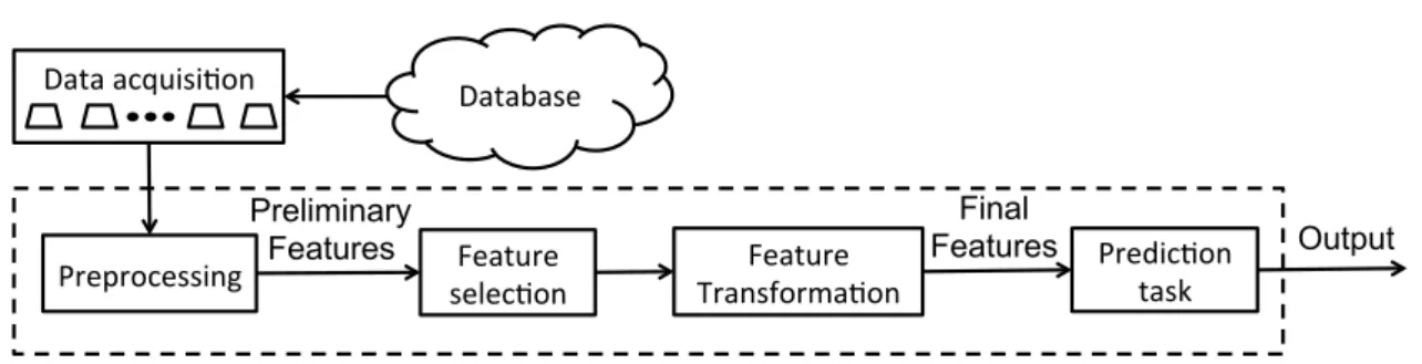
A flowchart illustrating the steps it takes for a machine to complete its mission can be found in Fig. 1.1. Data acquisition is the first step into our data adventure. It usually refers to the actions that a user takes to retrieve and manipulate data from a database. After the query and formatting, an initialization called preprocessing is applied to clean up data and construct a preliminary feature space. This is a domain specific process that requires knowledge of information extraction for applications from different disciplines, such as speech analysis, image processing, medical appli-cations, text sentiment analysis, etc. The output of the preprocessing are called the preliminary features, which are then fed into the next step for further processing. Feature selection [3, 4] is a step that selects a subset of the preliminary features by removing redundant information, such that the computational complexity and stor-age requirement can be reduced. Of course, this subset selection intends to preserve
Feature
selec+on Transforma+on Feature Predic+on task Data acquisi+on Preprocessing Preliminary Features Database Final Features Output
Figure 1.1: A framework for learning a classification rule.
the informative structure of the original data. A subsequential block after feature selection is the feature transformation step, where instead of choosing a subset, the features are transformed onto a high dimensional space and then possibly restricted to a subspace of lower dimension. The purpose of this transformation is to create a new feature space by a linear or nonlinear combination of the selected features. The resulting features are then used as the input for the prediction task as illustrated in the previous paragraph.
Given different machine learning frameworks, Fig. 1.1 is modified accordingly. For instance, the Convolutional Neural Networks (CNN), one of the most popular deep learning techniques for image processing, integrates the three blocks (“Preprocessing”, “Feature selection” and “Feature transformation”) into one procedure to determine final features using a deep network. On the other hand, the classic Artificial Neural Networks (ANN) has a learning structure such that feature selection, feature trans-formation and the classifier are all implemented as a part of the backpropagation algorithm. Some other techniques, such as the Principal Component Analysis (PCA) with sparse representations [5, 6], perform feature selection and transformation si-multaneously.
1.2
Learning Process
In order to construct a machine that automatically performs prediction on its own as shown in Fig. 1.1, a learning process is needed for each block. Before the learning begins, We need to determine the following components:
• Model selection: It refers to choosing an appropriate family of learning models for a given machine learning task. In other words, the learning space is restricted to the selected model family. The learning model contains unknown parame-ters, which need to be estimated during the learning process. Moreover, model selection typically involves selecting hyperparameters within the model family, which are the parameters that one needs to know in advance to be able to solve for the unknowns. For instance, the number of principal components in PCA, the number of hidden layers and units in a neural net, the prior information in a Bayesian framework, etc. These hyperparameters are usually determined manually by the designer, but they can also be automatically selected using
1.3. Kernel Techniques machine learning techniques as well. This is sometimes called “metalearning”, since it is “learning” for the learning process.
• Learning objective: It is the mathematical formulation of the goal that the machine is expected to achieve. Typically, it is presented as an optimization problem, such as minimizing the squared error in linear regression. Constraints are often applied to further restrict the searching space in addition to the se-lected family of learning models. As an example, the learning objective of Support Vector Machines (SVM) is to find a hyperplane that maximizes the “margin” of the separation on the training data.
• Searching algorithm: Given the learning model and the objective with some constraints, the searching algorithm estimates the unknown parameters in the learning model. The formulation of the learning objective heavily affects the ef-ficiency and optimality of the searching process. For example, if an optimization problem is impossible to solve in polynomial time, or suffers from local optima, searching for the exact solution would be extremely time consuming and diffi-cult. On the other hand, if the learning objective is a convex problem, various existing tools would be available for finding the global optimal solution. Hence, tradeoffs are often being made while designing machine learning algorithms. The learning process can be categorized into supervised learning and unsupervised learning. The goal of supervised learning is to determine the intrinsic data structure and learning rules given both data and their labels for classification tasks or correct numerical outputs for regression. On the other hand, unsupervised learning does not require the label information [2]. Unsupervised learning refers to techniques such as k-means for automatic data clustering [7, 8].
Since the labels are visible to the machine for supervised learning, the parameter estimation is also called training, as it resembles the learning process trained by a supervisor. In this case, the data-label pairs are calledtraining data. This thesis work focuses on the development of supervised learning techniques.
1.3
Kernel Techniques
The kernel method [9, 10, 11, 12] is one of the most popular nonlinear learning tech-niques, which is based upon the construction of a high (possibly infinite) dimensional feature space endowed with an inner product. Learning techniques are applied in this constructed feature space accordingly. By using kernel techniques, the advantage is twofold:
- The high dimensionality of the constructed feature space provides the possibility of describing complex data structures;
- All computations are carried out by the kernel function on the original data. In other words, no explicit computations are required in the high dimensional feature space.
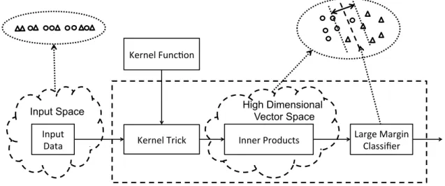
A Demonstration Using Kernel SVM
To gain a better intuition, we demonstrate kernel methods using the Support Vector Machine (SVM), which is also known as the maximal margin classifier. We try to limit this introduction to its minimum. One can find more detailed descriptions from, e.g. [13, 14, 11], and the references therein.
High Dimensional Vector Space
Kernel Trick Inner Products Large Margin Classifier Input
Data
Kernel Func;on
Input Space
Figure 1.2: A flowchart of kernel SVM.
Soft Margin SVM: First, let us leave kernels aside and focus on the formulation of SVMs. In a classification problem, a SVM tries to find a hyperplane that separates data from two classes with the largest margin. There are two types of margins: the
hard margin and the soft margin. Different margins reflect different concerns, which result in their own distinct formulations. Briefly speaking, a hard margin can only be used when training data are linearly separable, whereas soft margin allows some misclassified data points during training. In fact, soft margin is more commonly used in practice due to its robustness [15].
In Fig. 1.2, a soft margin is illustrated in the picture above the “Large Margin Classifier”. It is defined as the distance between the dashed line (the separating hyperplane) and the dotted line (the marginal hyperplane). Mathematically speaking, this distance can be computed using the length of the perpendicular vector (usually denoted as w) that connects these two lines, i.e. 1
kwk2. Due to the symmetry of the two marginal hyperplane and also for optimization convenience, one uses kw2k2
2 to denote the margin, i.e. the distance between the two marginal hyperplanes. In other words, every vector w defines a hyperplane that separates the data space into two disjoint half-spaces.
Now, given a training set n
(xi, yi) :xi ∈Rp;yi ∈ {−1,+1};i= 1,· · · , N;p, N ∈N+
o
,
1.3. Kernel Techniques a bias b∈R such that [13]:
minimize: w,b 1 2kwk 2 2+η X j ξj subject to: wTϕi+byi ≥1−ξi, ∀i ξi ≥0, ∀i (1.1)
where ξi is called the slack variable, which indicates the signed distance from a
mis-classified data point to the marginal hyperplane. The scalar η is chosen by the user to control the misclassification rate. Generally speaking, the smaller η is, the larger number of misclassified data are allowed during training.
More precisely, a given data pair (ϕ, y) is on the marginal hyperplane if and only if wTϕ +b =
+1, for y= +1
−1, for y=−1. Therefore, a unified expression for the marginal hyperplane is wTϕ+by = 1. In fact, for any (ϕ, y), the larger wTϕ+by is,
the better this data point is separated from the other class and the signed distance between the marginal hyperplane and (ϕ, y) is expressed by 1−wTϕ+by. Given
this analysis, the soft margin SVM can be interpreted as maximizing the margin, while minimizing the distance from the marginal hyperplane to the misclassified training data, i.e. data that satisfy 1−wTϕ
i+b
yi ≥0.
Duality: To solve the optimization problem in Eq. (1.1), one possibility is to analyze its duality. By computing the Lagrangian [16] and its KKT condition, we obtain the dual of Eq. (1.1): maximize: α X j αj− 1 2 X i,j αiαjyiyjϕTi ϕj subject to: X i αiyi = 0 0≤αi ≤η, ∀i (1.2)
whereαis the vector that contains the Lagrangian multipliers and αi denotes the ith
element ofα. Moreover, the KKT condition results in the following relation between the normal vector wand Lagrangian multipliers:
w=X
i
αiyiϕi (1.3)
In other words, the normal vectorwcan be written as a linear combination of training vectors ϕi’s.
Kernel Trick: When the dimension of ϕi’s is high, the computation of ϕT
i ϕj can
be prohibitive. In kernel techniques, one reduces the computational complexity by a technique called the “kernel trick”.
Letxi,xj be any data points sampled from the low dimensional input space. Now
let us define a “kernel function” k, such that
k(xi,xj),ϕTi ϕj, (1.4)
which means that the computation ϕT
iϕj can be carried out in the low dimensional
input space Rp. Eq. (1.4) is called the kernel trick in the literature. Briefly speaking, the kernel trick utilizes the kernel function k to produce computations in the high dimensional space, where the classifier is established. This is an efficient replacement since inner products ϕT
i ϕj are all the computations we need in the high dimensional
space for SVM to estimate the unknown parameters αi’s.
Furthermore, when applying the classifier to an unseen data vector ˜x, one has to evaluate the following:
f(˜x),wTϕ(˜x) =X i αiyi ϕTi ϕ(˜x) | {z } kernel trick =X i αiyik(xi,x˜) (1.5)
such that the estimated label ˆy for ˜xis computed as: ˆ y= +1, f(˜x)≥0 −1, f(˜x)<0 (1.6) where again, no high dimensional computation is needed in Eq. (1.5).
To summarize, in kernel techniques, the original low dimensional data are mapped onto a high dimensional feature space using the kernel function to gain better flexibil-ity, whereas no explicit high dimensional computation is needed thanks to the kernel trick.
1.4
Challenges
When designing a machine learning system, the selection of the most appropriate family of learning models is not a trivial task. Various trade-offs need to be taken into consideration.
1.4.1
Bias and Variance
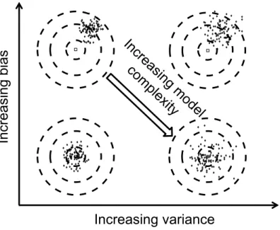
Given a learning system, estimations for unknown parameters vary with respect to different training sets. The bias and variance can be computed accordingly for esti-mated parameters and/or the prediction output. Empirically, the bias and variance can be approximated using the sample mean and the sample variance, respectively. A demonstration can be found in Fig. 1.3. Generally speaking, the trade-off between bias and variance is related to the model complexity. That is, learning models with high complexity tend to have low bias but high variance, and vice versa. Hence, the trade-off can be found by choosing a model family that is suitable for the problem at hand [17].
1.4. Challenges
In
cre
asi
ng
b
ia
s
Increasing variance
Incre
asi
ng
mo
de
l
co
mp
lexi
ty
Figure 1.3: A visualization of bias/variance with increasing model complexity. The example shows the estimation of the expected value for some given training sets. With increasing complexity, the bias of the estimate decreases whereas the variance will increase.
Example 1.1 (Kernel function and bias-variance trade-off for SVMs). As shown in Eq. (1.4), the kernel function k(·,·) defines an inner product as a nonlinear function of the input data. This is equivalent to constructing a nonlinear map ϕ(x), such that
ϕ : x 7→ ϕ for any input data x, where ϕ is a high dimensional vector. Hence, by using the kernel function k(·,·), the higher dimensional ϕ is, the higher complexity the corresponding SVM has. In other words, when working with SVMs associated with “simple” kernel functions 1, one expect high bias with low variance, and vice versa.
1.4.2
Robustness
There are mainly two aspects when it comes to the robustness of machine learning algorithms:
• Overfitting: It refers to the problem of a learning system lacking generalization ability, which is indicated by achieving a low fitting error on the training data but suffering from inaccurate prediction on unseen testing data.
• Noise/error handling: Given a learning system, the prediction accuracy will vary with increasing noise level or measurement error. The robustness from this perspective can be interpreted as the smoothness and stability of the system. Example 1.2 (Soft margin SVM and its robustness). First, we introduce the hard margin SVM. A hard margin SVM is applied when the training data are linearly
1Here a simple kernel function refers to a kernel function corresponding to a low dimension ofϕ. Detailed description can be found in Chapter 2
separable. Intuitively speaking, one attempts to find a separating hyperplane f char-acterized by its normal vectorw=PN
i=1αiϕ(xi), such that i)f categorize all training data to their correct classes; ii) αi’s are only nonzero for a subset of training data. Members in this subset is called “Support Vectors”. More precisely, the support vec-tors are the data points located on the marginal hyperplane. However, a hard margin does not take into consideration the presence of noise. It completely depends on a specific subset of training data. In particular, if the training size is small, hard mar-gin SVMs are especially prone to overfitting. A soft marmar-gin SVM, on the other hand, finds a separating hyperplane in a weighted consensus fashion. That is, if a well classified data point is “far away” from the marginal hyperplane, its contribution to constructing the classifier is small, whereas the more “ambiguous” a data point is, the higher weight it has. The weighting is controlled by the hyperparameterη in Eq.(1.1). Therefore, in the soft margin SVM, values for αi’s are more smooth compared to the hard margin SVM, which introduce better robustness to the learning process.
1.4.3
Scalability
The scalability in machine learning usually refers to the computational complexity and/or the storage requirement for training, which can be improved by the following:
1) using approximations instead of exact solutions;
2) choosing the most suitable programming language with efficient coding scheme; 3) taking advantage of parallel/distributed frameworks;
4) exploiting appropriate data structures;
5) finding the trade-off between computational complexity and storage usage. Example 1.3 (Scalability of SVM). From the formulation of the soft margin SVM (c.f. Eq.(1.2), there are mainly three concerns regarding the scalability that one should take into account:
- Different computational complexity caused by different kernel functions;
- Kernel matrix for large training size;
- Training time with respect to η for large training size N.
1.4.4
Hyperparameter Tuning
Hyperparameters refer to the parameters in the learning model that is not part of the variables that the training algorithm is solving for. Typically, their values need to be set manually prior to the learning process. Hyperparameter tuning can be con-sidered as an outer training loop and it needs to be validated by unseen testing data. Generally speaking, the more hyperparameters there is, the more flexible the model
1.5. Conclusion is due to the high degrees of freedom. However, one needs to be cautious that high flexibility often implies high complexity, which might lead to high variance. Moreover, when the number of hyperparameters is large, the evaluation of their quality requires high computational complexity and its “optimality” typically lacks theoretical justi-fication. Hence, one needs to be aware of the trade-off between the flexibility and the number of hyperparameters.
1.5
Conclusion
In this chapter, we have given a brief introduction on the subject of machine learning, where the learning process is decomposed into three components: 1) model selection, 2) learning objective and 3) the searching algorithm. Kernel method is then intro-duced as one of the most popular nonlinear learning techniques and the main con-cept is illustrated using the Support Vector Machines. Moreover, we have identified challenges and trade-offs when designing kernel techniques, which gives rise to the potential areas for further development.
Chapter 2
Reproducing Kernel Hilbert Space
and its Application
In this chapter, the theoretical background of kernel techniques is introduced. We start with the preliminaries for the definition of the Reproducing Kernel Hilbert Space and its properties, which leads to its applications for solving machine learning problems.
Given an input spaceX ×Y, whereX is a non-empty input set that consists of any objects, such as numerical vectors, texts, images, DNA strings, pages of websites, etc. The setY typically contains scalars that takes either discrete values for classification, or continuous values for regression. The underlying assumption is that the intrinsic distribution of such random objects is “well” represented in a high dimensional feature space F that can be obtained by a nonlinear feature mapϕ:X → F.
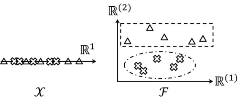
The effectiveness of such transformations mainly results from the increased di-mensionality, i.e. dim(F)dim(X). To illustrate, let us consider the classification problem shown in Fig. 2.1, where the “wishful” results is achieved by applying a non-linear transformationϕ(·) to a one dimensional input space, such that feature vectors from different classes in the resulting feature space F =R2 are “better” separated.
!
!
ℱ!
ℝ
!!
ℝ
(!)!
ℝ
(!)!
Figure 2.1: A demonstration of the nonlinear mapping ϕ : X → F. The crosses and triangles represent data vectors from two different classes. In order to perform classification, the class separability, visualized by the Euclidean distance between the two clusters, is clearly better in the high dimensional space F.
some fundamental concepts and definitions in Sec. 2.1, we illustrate the theory be-hind reproducing kernels and the associated feature spaces. Essentially, the message of Sec. 2.2 is that for every positive definite kernel function there exists a unique Reproducing Kernel Hilbert Space (RKHS), where the inner product is well defined. There also exist other feature spaces that are isometrically isomorphic to the RKHS associated with the same kernel function. Examples of commonly used kernel func-tions and the construction of feature spaces are then demonstrated. Given the core concepts of kernel techniques, practical issues on optimization in feature spaces are addressed in Sec. 2.3.
2.1
Brief Review on Functional Analysis
In this section, we give a brief introduction on the subject of Reproducing Kernel Hilbert Space (RKHS). An inner product space induces a metric space, which is endowed with a corresponding distance metric used as a similarity measure. In kernel techniques, one constructs an inner product space H with some extra properties and uses H as the feature space for learning. Typically, the dimensionality of H is very large or even infinite. A kernel function k : X × X → R is applied to replace the explicit computation of inner products in H. In fact, the space H is completely characterized by the kernel function, which allows us to work in the original space X instead of the high dimensional space H. Since operations are not directly carried out in the RKHS, the properties ofHis rather unclear to us, especially in the infinite dimensional case. Hence, to gain better understanding, one has to borrow some tools from mathematical analysis.
This section is fairly self-contained, but we assume a basic familiarity with the fundamental concepts in functional analysis, such as metric space, normed vector space, completeness, etc. Throughout this presentation, the field of the scalars for the vector space is the field of real numbers R.
2.1.1
Hilbert Space
One of the most important concept for a vector space is its basis.
Definition 2.1 (Basis). A basis of a (finite or infinite dimensional) vector spaceV is a linearly independent subset {e1,e2,e3,· · · }of vectors that span V. Equivalently, a
subset {e1,e2,· · · } is a basis if and only if every v∈ V can be uniquely written as
v=a1ei1 +· · ·+anein
where a1,· · · , an ∈Rfor some finite n ∈Z+ and ij ∈Z+ for 1≤j ≤n.
The definition implies an important property for a subset being a basis: the finiteness in the linear combination for representing any vectors in that space. The existence of a basis for any finite dimensional vector space is obvious, whereas it is less clear in the infinite dimensional case. In fact, by accepting Zorn’s Lemma (or equivalently, the axiom of choice), one can claim that every vector space has a basis.
2.1. Brief Review on Functional Analysis
Lemma 2.1(Zorn’s Lemma).IfX is a partially ordered set and every linearly ordered subset of X has an upper bound, then X has a maximal element.
To show that every vector space has a basis, let T be a collection of all linearly independent subsets of a vector spaceV. We then order the elements inT by inclusion E1 ⊂ E2 ⊂ · · ·. Hence, the union of the chain, denoted byU, also belongs toT due to
the definition of T. Now we have found ourselves an upper bound, U. By accepting Zorn’s Lemma, we know that there is a maximal linearly independent set M in T. To show M is a basis for V, we have to show that this maximal set spans V. This is easily proven by contradiction. Assume that there is a element v∈ V, such that v is linearly independent of all vectors inM, then we haveM ⊂ M∪v, which contradicts the maximality of M.
In particular, whendim(V) is infinity, the basis is called the Hamel basis.
While the existence of a basis in any vector space does sound comforting, Zorn’s Lemma is not quite useful, i.e. it does not provide any construction of the basis. In fact, there is no practical way of finding a Hamel basis in general. This gives rise to the importance of the orthonormal basis, where infinite sums of linearly independent vectors are allowed to represent a vector. Moreover, for the infinite sum to make sense, one needs the definition of convergence on the vector space, which requires the notion of topological vector spaces. This brings us to the definition of the inner product space. Note that we have neglected the definitions of other important objects, such as metric spaces and normed vector spaces, since they are naturally induced by inner product spaces.
Definition 2.2 (Inner Product). Let H be a vector space. An inner product on H is a map (v,u)→ hv,uiH from H × H →R such that:
• hau+bv,ziH =ahu,ziH+bhv,ziH, for all u,v,z∈ H and a, b∈R.
• hv,ui=hu,vi, for all u,v∈ H. • hu,ui ∈(0,∞), for all nonzero u∈ H.
It is obvious that every inner product induces an associated normkuk=qhu,uiH and thus convergence can be defined accordingly. Without ambiguity, unless neces-sary, we simply denote the inner product and the induced norm using h·,·i and k · k, respectively, without specifying the corresponding vector space.
Definition 2.3 (Pre-Hilbert Space). A vector space equipped with an inner product is called an inner product space, or a pre-Hilbert space. One advantage of an inner product space over a normed space is that an inner product space allows us to define orthogonality.
Definition 2.4 (Orthogonality). Given a pre-Hilbert space H0 and u,v ∈ H0, we
say u and vare orthogonal, denoted as u⊥v, if hu,vi= 0.
Some well-known inequalities and identities are listed below. They are frequently applied for various proofs in a pre-Hilbert spaces.
• Cauchy-Schwartz Inequality:
|hu,vi|2 ≤ hu,ui · hv,vi (2.1)
• Triangle Inequality:
|hu+vi| ≤ kuk+kvk (2.2)
• The parallelogram law:
kuk2+kvk2 = 1
2
ku+vk2+ku−vk2
(2.3) • The polarization identity:
hu,vi= 1 4
ku+vk2− ku−vk2 (2.4)
• Pythagorean Theorem: If u⊥v, then
ku+vk2 =kuk2+kvk2 (2.5)
An inner product space without any extra properties is called a pre-Hilbert space for a reason: a Hilbert space is the “comfort zone” for analysis and to construct a Hilbert space from a pre-Hilbert space, there is just one step missing.
Definition 2.5 (Hilbert Space). A Hilbert space H is a pre-Hilbert space that is complete with respect to the norm kuk=qhu,ui, for u∈ H.
To understand completeness, one has to recall the definition of a Cauchy sequence. Definition 2.6(Cauchy sequence). Given a metric space (M, d), a sequenceu1,u2,u3,· · ·
is called Cauchy if d(um,un)→0 as m, n→ ∞.
Letd be the distance metric induced by the norm k · kH, then
Definition 2.7 (Completeness). Completeness means that every Cauchy sequence in H converges to a limit that is also in H.
Intuitively, a space being incomplete means that it has “holes” in it, i.e. not every seemingly convergent sequence is converging to a point inside the space. Obviously, that is problematic when we try to find a nice space to analyze infinite sums. Nev-ertheless, the completion does not take much extra effort. That is, to complete a pre-Hilbert space, one simply adds the limit points of sequences that are convergent in that norm. In other words, to reach any point in a Hilbert space, one simply constructs a Cauchy sequence converging to that point.
Note that for the remainder of the chapter, we useH to denote Hilbert space. Remark. Any closed subspace of a Hilbert space is itself a Hilbert space.
2.1. Brief Review on Functional Analysis One important feature of a Hilbert space is that it enables the concept of projec-tions.
Theorem 2.1. If M is a closed subspace of H, then H = ML
M⊥; that is, each u∈ H can be expressed uniquely as u=y+z where y∈ M and z∈ M⊥. Moreover, y and z are the unique elements of M and M⊥ whose distance to u is minimal.
To characterize a Hilbert space and its subspaces, we introduce the definition of a basis for infinite dimensional space.
Definition 2.8 (Orthonormal Set). A subset {uα}α∈A of H is called orthonormal if
kuαk= 1 for all α and uα ⊥uβ whenever α6=β, where A is some index set.
Theorem 2.2. If {uα}α∈A is an orthonormal set inH, the following are equivalent:
• (Completeness) If hz,uαi= 0 for all α, then z= 0.
• (Parseval’s Identity) kzk2 =P
α∈A|hz,uαi|2 for all z∈ H.
• For each z ∈ H, z = P
α∈Ahz,uαiuα, where the sum on the right has only countably many nonzero terms and converges in the norm topology no matter how these terms are ordered.
Definition 2.9 (Orthonormal Basis). An orthonormal set having the properties in Theorem 2.2 is called an orthonormal basis.
Theorem 2.3 (Separable Hilbert space). Every Hilbert space has an orthonormal basis and a Hilbert space H is separable iff it has a countable orthonormal basis, in which case every orthonormal basis is countable.
When H is separable (i.e. H contains a countable dense subset), a standard procedures can be applied to obtain an orthonormal basis. Given {xn}∞1 a linearly
independent subset in H, we recall two such methods: • Gram-Schmidt process
– Letu1 = kxx11k;
– Having defined{u1,· · · ,uN−1}, setvN =xN−PNn=1−1hxN,ununi, anduN =
vN
kvNk;
– The resulting set{u1,u2,· · · } is then an orthonormal basis forH.
• Principal Component Analysis
LetXbe a matrix withxias itsithcolumn, for 0< i≤ ∞. A set of orthonormal
vectorsu1,u2,· · · are called the Principal Components of a spaceH ifuk is the
kth eigenvector of matrix XXT, where indices k’s are sorted with respect to
eigenvalues of XXT in a descending order.
Note that in the literature, separability is usually assumed for Hilbert spaces. In fact, as Folland [18] has pointed out, “most Hilbert spaces that arise in practice are separable”. However, the separability is not a property that a Hilbert space possesses automatically. Interested readers can refer to [18, 19] for more fundamental proofs and discussions.
2.1.2
Riesz Representation Theorem
The Riesz Representation theorem is one of the most fundamental results in functional analysis of Hilbert spaces and it provides tools for proving and analyzing the existence and uniqueness of a RKHS and its associated kernel function.
Definition 2.10 (Linear functional). Given Hilbert spaceH, a functionT :H → R is called a linear functional if
T (au+bv) = aT(u) +bT(v) (2.6) where u,v∈ H and a, b∈R.
Definition 2.11 (Bounded). A linear functional T : H → R is called bounded if there exists C≥0 such that |Tu| ≤CkukH, for all u∈ H.
Definition 2.12 (Continuous). If u ∈ H, linear functional T is called continuous at u if for every neighborhood O of T(u) there is a neighborhood U of u such that
T(U)⊂O. In particular, the functional T is called continuous iff T is continuous at every u∈ H.
Proposition 2.1. For a linear functional T :H →R, the following are equivalent:
• T is continuous on H.
• T is continuous at 0.
• T is bounded.
So far we have been talking about linear functionalT, the domainH of T, andT
being continuous/bounded.
Definition 2.13 (Dual Space). The space of bounded linear functionals on H is called the dual space of H and is denoted by H∗.
Remark. The dual space of a Hilbert space is a Hilbert space itself.
Theorem 2.4 (Riesz Representer Theorem). If f ∈ H∗, there is a unique u ∈ H,
such that f(v) = hv,ui for all v∈ H.
The Riesz Representation theorem has established the relation between a Hilbert space and its dual through the inner product. It is an essential tool to show the existence and uniqueness of the kernel function on an RKHS.
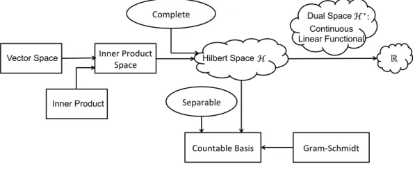
The key concepts introduced in this section can be found in Fig. 2.2. To summa-rize, a Hilbert space is a complete vector space that endowed with an inner product. Completeness secures the analysis. For instance, completeness makes sense of limits in that space. Compared to Banach spaces, which are complete normed vector spaces, Hilbert spaces come with a natural definition of orthogonality and projection. Fur-thermore, by imposing separability, we can construct a countable orthonormal basis by using the Gram-Schmidt process. The dual space of a Hilbert space is defined as the space of all the continuous linear functionals, which is in fact a Hilbert space itself.
2.2. Reproducing Kernel Hilbert Space (RKHS) and Feature Maps Vector Space Inner Product Inner Product Space Complete Hilbert Space ℋ! ℝ! ℋ∗:! Dual Space Continuous Linear Functional Separable
Countable Basis Gram-‐Schmidt Figure 2.2: A summary of Sec. 2.1.1 and Sec. 2.1.2.
2.2
Reproducing Kernel Hilbert Space (RKHS) and
Feature Maps
2.2.1
Reproducing Kernels
Definition 2.14 (Reproducing Kernel Hilbert Space (RKHS)). Given a non-empty setX, a Reproducing Kernel Hilbert Space (RKHS) is a Hilbert space Hof functions
f : X → R with a reproducing kernel whose span is dense in H. Specifically, a function k :X × X →R is called a reproducing kernel of H if k satisfies:
• ∀x∈ X, k(x,·)∈ H;
• (The reproducing property) ∀x ∈ X, hf, k(x,·)i = f(x), for all f ∈ H. In particular, hk(x,·), k(˜x,·)i=k(x,x˜).
The span of the reproducing kernel being dense means thatk(x,·) spansH. Note that we reserve the notation H to denote a Reproducing Kernel Hilbert Space.
From the Riesz Representation theorem, we know that givenf ∈ H, if there exists a function k(x,·)∈ H, such thatf(x) =hf, k(x,·)i, then k(x,·) must be unique. Remark. For a given reproducing kernel k and x,x˜ ∈ X, let H be the RKHS associated with the function k. We have the following clarification on the notions:
• k(x,·) :X → H is a function of x, i.e. we can define a nonlinear map ϕ:X → H, such that ϕ(x) = k(x,·). Also, we can viewk(x,·) as a vector in the RKHS. • k(x,x˜) is a scalar, i.e. k(x,x˜) =hk(x,·), k(˜x,·)iH =hϕ(x), ϕ(˜x)iH, due to the
reproducing property.
• Every function f ∈ H can be written as a linear combination of feature maps, i.e. f(·) = m X i=1 αik(xi,·) (2.7)
where αi’s are coefficients. It directly follows that
hf, k(x,·)i= h m X i=1 αik(xi,·), k(x,·)i = m X i=1 hαik(xi,·), k(x,·)i = m X i=1 αik(xi,x) (2.8)
where m∈N and αi’s are coefficients.
Example 2.1. Denote xi = " x1 i x2 i #
for any index i, let k(xi,·) =
x1i x2 i x1 ix2i . For all
x1,x2,x3,· · · ∈R2 The span of k(x,·) would be the space spanned by
{k(x1,·), k(x2,·),· · · }= x1 1 x2 1 x1 1x21 , x1 2 x2 2 x1 2x22 ,· · ·
The representer k(x,·) can be interpreted as the nonlinear map ϕ:R2 →R3.
Definition 2.15 (Positive Definite (PD) kernel). A real-valued symmetric function
k :X ×X →Ris called a positive definite (PD) kernel if for alln ≥1,x1,· · · ,xn∈ X,
c1,· · · , cn ∈R
n
X
i,j=1
cicjk(xi,xj)≥0 (2.9)
Theorem 2.5 (Moore-Aronszajn Theorem [20]). To every positive definite function
k onX × X there corresponds a unique RKHS of real valued functions on X and vice versa.
Theorem 2.5 is one of the most fundamental results in kernel methods. It guaran-tees the existence and uniqueness for the RKHS and its corresponding kernel function. In other words, by defining a PD kernel function, a unique RKHS is generated au-tomatically. The function norm in the RHKS k · kH is thus induced by the kernel function.
2.2.2
Kernel Functions
As stated above, given a positive definite kernel function, we do not have to worry about the existence of the corresponding RHKS. The question is then which functions are positive definite functions.
2.2. Reproducing Kernel Hilbert Space (RKHS) and Feature Maps
Examples of Kernel Functions:
• Linear kernel: k(x,x˜) = xTx˜ (2.10) • Polynomial kernel: k(x,x˜) = (hx,x˜i+c)d, c∈R+ 0, d∈Z + (2.11) • RBF kernel: k(x,x˜) = exp −kx−x˜k 2 2 2σ2 ! , σ∈R+ (2.12) • Sigmoid kernel:
k(x,x˜) = tanhaxTx˜+b, a, b∈R+, x real valued vector (2.13)
• Sinc kernel:
k(x,x˜) = sin (kx−x˜k2) kx−x˜k2
(2.14) • String kernels [21]: Given an alphabet Σ, a string s is a finite sequence of characters from Σ with cardinality |s|. Let u be a subsequence of s, i.e. there exists indices{i(1),· · · , i(|u|)} sorted in ascending order, such thatuj =si(j), for
j = 1,· · · ,|u|, where |u|<|s|. Denotes[i] :=u andl(i) :=|s[i]|. Let Σn be the
set of all finite strings of length n and by Σ∗ be the set of all strings Σ∗ =
∞
X
n=0
Σn
The feature mapping for a string s is given by defining theu coordinate ϕu(s)
for each u ∈Σn. Define ϕ
u(s) =Pi:u=s[i]λl(i), for some λ ≤1. Given strings s
and t, the kernel function is then defined as:
kn(s, t) = X u∈Σn hϕu(s), ϕu(t)i = X u∈Σn X i:u=s[i] λl(i) X j:u=t[j] λl(j) = X u∈Σn X i:u=s[i] X j:u=t[j] λl(i)+l(j)
It turns out that the string kernel can be efficiently evaluated using dynamic programming techniques [21]. One example is shown in Tab. 2.1. The kernel between the work “car” and “cat” is k(car,cat) = λ4. Since k(car,car) =
k(cat,cat) = 2λ4+λ6, the normalized kernel is:
k(car,cat) q
k(car,car)qk(cat,cat) = 1 2 +λ2
c-a c-t a-t b-a b-t c-r a-r
ϕ(cat) λ2 λ3 λ2 0 0 0 0
ϕ(car) λ2 0 0 0 0 λ3 λ2
ϕ(bat) 0 0 λ2 λ3 λ2 0 0
Table 2.1: An example of string kernel
Combination of Kernel Functions:
Let k1 and k2 be two PD kernel functions, then the following functions are also valid
PD kernel functions:
- k(x,x˜) = ck1(x,x˜),c∈R+
- k(x,x˜) = f(x)k1(x,x˜)f(˜x), where f :X →R
- k(x,x˜) = p(k1(x,x˜)), where p(·) is polynomial with non-negative coefficients
- k(x,x˜) = expk1(x,x)˜ σ2 ,σ ∈R - k(x,x˜) = exp−k1(x,x)−2k1(x,x)+˜ k1(˜x,˜x) σ2 , σ ∈R - k(x,x˜) = k1(x,x˜) +k2(x,x˜) - k(x,x˜) = k1(x,x˜)k2(x,x˜)
- k(x,x˜) = xTAx˜, whereA is a symmetric PSD matrix - k(x,x˜) = (k1(x,x˜) +c)d, where c∈R+ and d∈Z+
- k(x,x˜) = √ k1(x,x)˜
k1(x,x)k1(˜x,x)˜
, normalization of kernel functions
Stationary Kernels k(x,x˜) = k0(|x−x˜|):
A kernel functionk(x,x˜) is called stationary or translation invariant if it is a function of only the distance between x and ˜x, i.e. k(x,x˜) = k0(|x−x˜|). For instance, the RBF kernel is stationary, whereas the polynomial kernel is non-stationary. Since a non-stationary kernel function depends on not only the relative relation, but also the position ofx and ˜x, coordinates need to be chosen to find the basis that describe the feature space. The origin is usually chosen to be the mass center of the training set [22].
k(x,x˜) ← (ϕ(x)−E(ϕ(x)))T (ϕ(˜x)−E(ϕ(˜x)))
2.2. Reproducing Kernel Hilbert Space (RKHS) and Feature Maps where E(ϕ(·)) can be estimated using the training data {x1,· · · ,xN}.
k(x,x˜)←k(x,x˜)− 1 N N X i=1 k(xi,x)− 1 N N X i=1 k(xi,x˜) + 1 N2 N X i=1 N X j=1 k(xi,xj) (2.15)
More information on the classification and properties of kernel functions can be found in [23, 24].
2.2.3
Constructing Feature Maps from Kernel Functions
For a given PD kernel function k, the existence and uniqueness of the RKHS is guaranteed. However, the construction of RKHS is not always convenient in practice. Fortunately, there exist other features maps ϕ:X → F for k(x,x˜) =hϕ(x), ϕ(˜x)iF, such that the inner product is preserved in the sense that H and F are associated with the same kernel function. Note that not every feature space is RKHS.
Example 2.2 (Feature spaces are not unique). Given any x,x˜ ∈ R2 with x =
" x1 x2 # and x˜ = " ˜ x1 ˜ x2 #
, let k(x,x˜) =x1x˜1+x2x˜2+ 2x1x2x˜1x˜2, we can construct the following
feature maps: - ϕ1(x) = h x1 x2 √ 2x1x2 iT - ϕ2(x) = h x1 x2 x1x2 x1x2 iT such that k(x,x˜) =hϕ1(x), ϕ1(˜x)i=hϕ2(x), ϕ2(˜x)i.
Nevertheless, feature space F and RKHS H are closely related, since they share the same kernel function k. More precisely,
Definition 2.16 (Isomorphism). Hilbert spaces H1 and H2 are said to be
isomet-rically isomorphic if there is a linear bijective map T : H1 → H2 such that
hu,viH1 =hTu, TviH2
Isomorphism preserves inner product between two Hilbert spaces. Clearly, all feature spaces associated with the same kernel function are isometrically isomorphic. In this section, we introduce three methods to construct the feature mapsϕ:X → F: 1) the RKHS map; 2) the Mercer map and 3) the kernel matrix decomposition.
- RKHS map:
Let k : X × X →R be a positive kernel function. According to Theorem 2.5, every positive definite kernel is associated with a unique RKHSH. The feature map is defined as k(x,·).
- Mercer Map:


![Figure 2.8: Figure 4.2 in [13]: The bound on the risk is the sum of the empirical risk and the confidence interval](https://thumb-us.123doks.com/thumbv2/123dok_us/1454599.2694606/49.892.293.702.177.512/figure-figure-bound-risk-empirical-risk-confidence-interval.webp)