Compensators and Diffusion
Approximation of Point Processes and
Applications
Xin Dong
Department of Mathematics
Imperial College London
Thesis presented for examination for the degree of
Doctor of Philosophy in Mathematics
of Imperial College London
Declaration
I certify that this thesis, and the research to which it refers, are the product of my own work, and that any ideas or quotations from the work of other people, published or otherwise, are fully acknowledged in accordance with the standard referencing practices of the discipline.
Copyright
The copyright of this thesis rests with the author and is made available under a Cre-ative Commons Attribution Non-Commercial No DerivCre-atives licence. Researchers are free to copy, distribute or transmit the thesis on the condition that they at-tribute it, that they do not use it for commercial purposes and that they do not alter, transform or build upon it. For any reuse or redistribution, researchers must make clear to others the licence terms of this work.
Acknowledgement
This thesis would not have been possible and my PhD life would not be so wonderful without support and love from many people.
Firstly I would like to express my deep gratitude to my supervisor Dr. Harry Zheng for his continuous and boundless support and encouragement throughout my PhD study. His advices and comments are very critical to this thesis.
My sincere thanks go to Dr. Angelos Dassios from Department of Statistics, London School of Economics. He generously shared his time, idea and experience with me. He advised and inspired me all these years.
I am deeply grateful to Department of Mathematics at Imperial College. I en-joyed various well-organized reading groups, seminars and courses. I also benefitted from interesting discussions with many staff members in the Mathematical Finance section. I appreciate the companion and support from my lovely colleagues and friends in our Department: Luke Charleton, Dr. Wang Han, Dr. Kai Li, Yusong Li, Cong Liu, Daphne Liu, Francesco Mina, Benoit Pham-Dang, Patrick Roome and etc.
My special thanks also go to the Risk Analytics team at Citigroup for the finan-cial support. The projects carried out provided me an opportunity to understand the practical finance world. Dr. Marco Polenghi, Mr. Rickard Brannvall and Dr. Lappas have been always supportive and helpful. My colleagues at Citigroup shared a lot of experience with me and brought me a lot of care and encouragement.
Finally, but most importantly, I cherish the unconditional love and support from my beloved parents; as well as Yi Xing, who has always been standing besides me with his companion and encouragement.
Abstract
In this thesis, we study two classes of point processes by analysing key properties and discussing applications in finance and insurance. The first point process studied was the default indicator process in credit risk modelling. We considered a pure jump L´evy process of finite variation for the asset value and an unobservable random barrier. The default time was defined as the first time the asset value falls below the barrier. Using the indistinguishable intensity process and the instantaneous likelihood process, we proved the absolute continuity of the compensator for the default indicator process, or equivalently, the existence of the intensity process of the default time. Moreover, we found the explicit representation of the intensity in terms of the distance between the asset value and its running minimal value, thus the intensity is an endogenous process, which sheds new light on the relationship between the intensity model and the structural model.
The second class of point processes is the Dynamic Contagion Process, which has intensities modelled with a shot-noise component describing the external impact and mutually-exciting jump components that describe the internal contagion effect. In the bivariate case, we found the stationarity condition with which we explored the diffusion approximation of the high frequency point process system and applied it in filtering. In the univariate case, we constructed a pure jump process derived from a dynamic contagion process and showed the weak convergence to a Cox-Ingersoll-Ross model (CIR) process. The pathwise approximation provides an alternative method of simulating the square-root processes and can be further extended to the approximation of the Heston model in option pricing.
Contents
Abstract 5
1 Introduction 12
1.1 Preamble . . . 12
1.2 Overview . . . 12
1.3 Organization of the Thesis . . . 16
2 A Pure Jump L´evy Structural Model with a Barrier of Incomplete Information 18 2.1 Introduction . . . 19
2.1.1 Basics of Credit modelling . . . 19
2.1.2 Basics of L´evy processes . . . 24
2.1.3 Motivation . . . 27
2.2 The Model and the Main Result . . . 28
2.3 Proof of the Main Theorem . . . 32
2.3.1 Compensators and Likelihood Processes under Different Fil-trations . . . 32
2.3.2 Spectrally Negative L´evy Process with Finite Variation . . . 37
2.3.3 L´evy Process with Finite Variation . . . 41
2.3.4 Indistinguishability of Likelihood Process and Intensity Process 44 2.4 Conclusion . . . 45
3 Introduction to Bivariate Dynamic Contagion Processes 47 3.1 Introduction to Point Process Modelling . . . 47
3.2 Introduction of Basics . . . 49
3.2.2 Markov Processes . . . 52
3.3 The BDCP Model . . . 54
3.3.1 Definition . . . 54
3.3.2 The Branching Structure . . . 58
3.4 Existence of Moments . . . 60 3.5 Exact Simulation of BDCP . . . 62 3.6 Graphic Illustration . . . 66 3.7 Conclusion . . . 66 4 BDCP Stationarity Analysis 68 4.1 Introduction . . . 68
4.2 Markov Property and Limiting Distributions . . . 70
4.2.1 Markov Property . . . 70
4.2.2 The Limiting Distributions . . . 73
4.3 The Stationary Distributions . . . 77
4.4 Stationary Moments . . . 83 4.4.1 Stationary Mean . . . 84 4.4.2 Stationary Variance . . . 84 4.4.3 Stationary Correlation . . . 87 4.5 Proof of Lemmas . . . 87 4.6 Conclusion . . . 91
5 BDCP Diffusion Approximation and Applications in Filtering 92 5.1 Introduction . . . 92
5.2 Diffusion Approximation of The BDCP . . . 96
5.2.1 High Frequency Events System . . . 97
5.2.2 Diffusion Approximation . . . 99
5.3 Kalman-Bucy Filtering with Diffusion Approximation . . . 103
5.3.1 Filtering with Observation (N1, N2) . . . 105
5.3.2 Filtering with Observation N1+N2 . . . 105
5.3.3 An Approximate Filter . . . 107
5.4 Applications . . . 110
5.4.1 Pricing Problem . . . 112
5.5 Proofs . . . 115
5.5.1 Proofs in Section 5.2 . . . 115
5.5.2 Proofs in Section 5.3 . . . 126
5.6 Conclusion . . . 129
6 Diffusion Approximation of UDCP and Alternative CIR Simula-tion Scheme 130 6.1 Introduction . . . 131
6.1.1 Univariate Dynamic Contagion Processes . . . 131
6.1.2 Basics of CIR Processes . . . 131
6.1.3 Basics of the Heston Model . . . 132
6.1.4 Simulation Issues . . . 133
6.2 Diffusion Approximation . . . 135
6.2.1 Scaled UDCP Intensity Processes . . . 136
6.2.2 Weak Convergence to CIR processes . . . 137
6.2.3 From Variance Processes to Asset Price Processes . . . 139
6.3 Approximation Simulation Scheme for CIR Processes . . . 141
6.4 Numerical Results . . . 142
6.5 Conclusion . . . 145
7 Conclusions and Future Research 146
List of Figures
2.1 The asset return processX as in Example 2.2.6, the distance process
X−X and the intensity processλ. The data used are (c,ν,σ,θ) = (−0.02,0.1,0.15,0.01). . . 33 2.2 The term structure of credit spread S(t, h): the asset return process
Xas in Example 2.2.6 with the data (c,ν,σ,θ) = (−0.02,0.1,0.15,0.01),
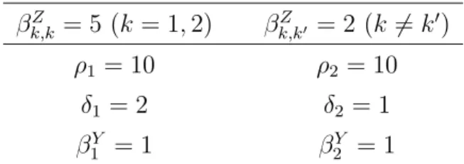
X−X at t=0.5 is 0.0585. . . 34 3.1 A simulated path of the BDCP and its intensity (N1, N2,λ1,λ2).
The self-exciting jumps !λk Tk j+−λ k Tk j "
j≥1 and cross-exciting jumps
! λk′ Tk j+−λ k′ Tk j " j≥1 for k, k ′ = 1,2 and k ̸=k′. . . . 67
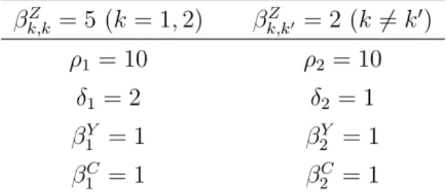
5.1 Observation scenario (S1): A sample path of λk
t compared with
its unconditional stationary mean and conditional estimate λk,Ft =
E[λk
t|σ{Ns1, Ns2, s≤t}] fork = 1,2. . . 111
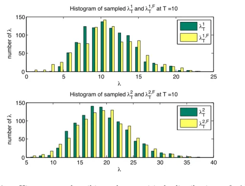
5.2 Histograms describing the empirical distribution ofλk
T andλkT|σ{Nt1, Nt2, t≤
T} denoted by λk,FT in the graph at T = 10 for k = 1,2. . . 112 5.3 Approximate solution of type estimationP#Ni
t ≤k|FN 1+N2 t $ at time t = 1. . . 115 6.1 A Sample path of a scaled UDCP intensity and a CIR process (with
different random seeds). . . 139 6.2 The Laplace transform of the integrated process with different
List of Tables
3.1 Parameters for the simulated path . . . 66 4.1 Notation of distributions in the branching system. . . 70 4.2 Coefficient table for A, B, C, ∆1 = δ1 −µG1,1 > 0 and ∆2 = δ2 −
µG2,2 >0. . . 85
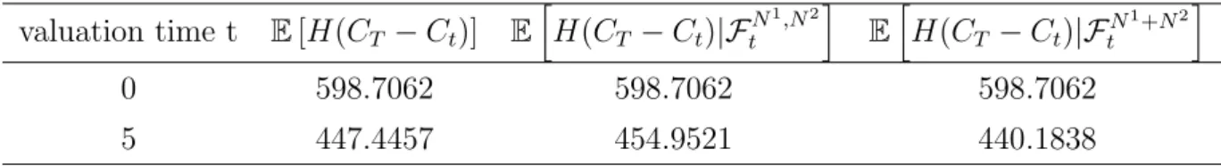
5.1 Parameters for numerical applications . . . 110 5.2 Comparison of the approximate conditional and unconditional
ex-pectations with T = 19.5. . . 113 5.3 Approximate stop-loss contract value of a given path of observation
(Nt1, Nt2), with H(x) = (x1+x2−d)+ with T = 19.5. . . 114
Notations
• (Ω,F,P) - the probability triple consisting of a sample space Ω, the σ-algebra
F which is the set of all measurable events, an the probability measure P.
• L2(P) - the set of all square-integrable random variables.
• (Ft)t≥0 - a filtration, that is an increasing family of sub-σ-algebras of F;
Fs ⊂Ft, 0 ≤s≤t.
• FX = (FX
t )t≥0 - the natural filtration generated by the process X.
• Rd - the d-dimensional Euclidean space.
• (DRd[0,∞),D) - path space of processes with c`adl`ag paths equipped the
Sko-rohod topology
• P - the probability measure on (DRd[0,∞),D) that is P =PX−1 induced by
process X.
• Xn ⇒X - weak convergence of process Xn toX in (D
Rd[0,∞),D)
• A, D(A) - the generator and its domain of a Feller process
• µHk,µiHk - the mean and the i-th (i≥2) moment of a random variable with
distribution H.
• UDCP - univariate dynamic contagion process
Chapter 1
Introduction
1.1
Preamble
A key challenge in many areas is how to model event arrivals in a system using a point process model that is able to capture a stylized fact. An understanding of key properties is needed to construct an appropriate point process model. In this dis-sertation, we will focus on the construction of appropriate point process models and study their probabilistic properties. The first model (M1) is for the default event of a firm. It aims to capture the short-term credit risk implied by the market and to explain the default risk in an economically meaningful way. The second model (M2) is a bivariate system for two-type event arrivals in a multi-name system with rich dynamics. We aim to study the stationarity property, investigate the diffusion approximation, and apply to solve filtering problems for the intensity process. The third model (M3) is a univariate pure jump process built on a univariate point process system for an approximate simulation algorithm of square-root diffusion processes.
1.2
Overview
(M1): A First Passage Time Model with Pure Jump L´evy Processes in Credit Modelling
An essential question in credit risk modelling is how to model the default time of a firm. The compensator of the default indicator process from the Doob-Meyer
decomposition presents rich information on the default time. For example, the regularity of the compensator conveys the extent of predictability of the default time. If the compensator is continuous, then the default time is totally inaccessible. Moreover, if it is absolutely continuous, then its Radon-Nikodym derivative with respect to the Lebesgue measure, called the intensity process, can be interpreted as the instantaneous default probability. In practice, it is also the short spread observed in the market, which quantifies the compensation an investor requires for bearing the short-term uncertainty of default. Ideally, we are looking for a model that can explain the reason for a firm’s default as well as the short-term default risk implied by the market.
There are three main modelling frameworks in the credit risk literature where the default time is defined differently. As a result, the probabilistic properties of default times are different. The first framework is the first passage time structural model (Black and Cox [12]) where the default time is the first time the asset price of the firm falls below a certain barrier. The model is economically meaningful as it explains the reasons for a firm’s default. However, the classical model using a geometric Brownian motion asset price and a constant barrier leads to a predictable default time. Hence, the intensity process does not exist, which contradicts market observations. The second framework is the intensity-based model (Lando [51]) where the intensity process is assumed to exist and is modelled by an exogenous process. This framework does not explain why a firm defaults. A third framework aims to bridge the gap between the above two main frameworks. It starts with a first passage time structural model and assumes incomplete information for market investors. It aims to show the existence of the intensity process. Duffie and Lando [29] and Kusuoka [49] assume a noisy accounting report on the asset price process and show the existence of the intensity process. Giesecke and Goldberg [36] and Giesecke [34] propose an unobservable random barrier and an observable geometric Brownian motion asset price process. They conclude that the intensity process does not exist as the compensator is not absolutely continuous.
In line with Giesecke [34], we propose an incomplete information first passage time structural model with an unobservable random barrier and an observable asset price process modelled by a L´evy process with finite variation. L´evy processes with finite variation, including the inverse Gaussian and the variance gamma models, are
widely used in price process modelling (Madan et al. [55] and Madan and Schoutens [56]) as they are able to capture some of the stylized facts of returns observed in the market and their probabilistic properties can be characterised explicitly. We show the existence of an intensity process based on the projection theory and the proper-ties of L´evy processes. Moreover, we find the explicit form of the intensity process that is an endogenous process depending on the parameters and the historical path of the asset price process. Therefore, the intensity explains the short spread ob-served in the market and it is dependent on the default mechanism. We therefore reconcile the structural model and the intensity model in credit risk modelling.
In this framework, the pricing formula can be derived which has an additional term (jump at default) compared to the classical formula in a Cox model. However it is difficult to calculate the additional term explicitly.
(M2): Bivariate Dynamic Contagion Processes
We model event arrivals in a two-type events system by a non-explosive bi-variate counting process with specified intensity processes. In order to reflect the idiosyncratic risk from some external factors and also internal contagion effects, we introduce the bivariate dynamic contagion process (BDCP) where the intensities are piecewise deterministic processes with external-exciting jumps and self-exciting jumps. The external-exciting jumps follow a compound Poisson process with an exponential time decay. The self-exciting jumps happen at the jump times of the counting process with a random jump size and an exponential time decay. There-fore, the BDCP is a generalized model of a bivariate Hawkes process (Hawkes and Oakes [39]) and a shot noise Cox process (Cox and Isham [19]).
We study a few key probabilistic properties of the BDCP. We find the station-arity condition under which there exists a stationary version of the process. Note that a BDCP is the limit of a sequence of finite branching systems in a cluster pro-cess representation. We first use Markov propro-cess theory to study, as time tends to infinity, the limiting distribution of a finite branching system in terms of a Laplace transform. We explore the condition to ensure the existence of the limiting distri-bution of the BDCP based on the convergence of the branching system. We show the limiting distribution is actually the stationary distribution and conclude that the condition found is the stationarity condition of the BDCP system.
due to the contagion effect. We study the diffusion approximation of the process which enables the application of more results available in the diffusion class. This is done using the martingale central limit theorem (Either and Kurtz [33]) and the stationarity result for the standardized intensity process. We obtain a limiting Gaussian system with the same mean and variance. Notice that the intensity in-formation is important but usually unobservable in practice, therefore we need to solve the filtering problem conditioned on the point process observations to get the best estimate of the intensity. Filtering with point process observations is discussed mainly in Br´emaud [13] and Ceci and Geraldi [15]. The innovation approach based on the martingale representation and the projection theory is used and the filter is proved to be a unique solution of the Kushner-Stratonovich (KS) equation. How-ever in general the KS equation can only be solved numerically. In this dissertation, we propose an efficient approximate solution to the filtering problem of the BDCP model. The solution proposed is a Kalman-Bucy filter of the limiting Gaussian diffusion process with actual point process observation inputs. Essentially, we ap-proximate not only the distribution but also the dependence structure of the point process system by the limiting diffusion process. We will show that the constructed filter is an asymptotically optimal filter. Moreover, we apply the diffusion approx-imation and the filtering solution in insurance for the pricing problem of stop-loss reinsurance contracts and the type estimation problem with numerical examples.
(M3): Pure Jump Processes for Approximate Simulation of CIR Pro-cesses
Due to the bias introduced by the negative value adjustment in the Euler sim-ulation method for CIR processes, alternative methods have been discussed in the literature. The exact simulation scheme based on the explicit form of the transi-tion probability of the CIR process is proposed, but it involves complicatransi-tions in sampling and is inefficient and sometimes even yields poor performance. The most popular method in practice is the Quadratic Exponential scheme (QE) introduced by Andersen [4]. The QE scheme is an approximate simulation scheme based on moment matching with a distribution that can be generated easily for the transition probability distribution. However, there is no convergence in this framework.
We propose an approximate simulation scheme for the CIR process with weak convergence results. We construct a pure jump process based on the univariate
dynamic contagion process (UDCP) and show the weak convergence to the CIR process when a model parameter tends to infinity using the martingale central limit theorem. Moreover, as the UDCP can be simulated exactly and efficiently, we obtain an alternative approximate simulation algorithm for the CIR processes. We conclude that the simulation scheme works well by comparing the Laplace transform of the simulated jump process with the theoretical value of the CIR process. As an extension, we can show that if we use the CIR process to model the stochastic volatility process of the asset, we obtain an approximate simulation scheme for the Heston model based on the weak convergence.
1.3
Organization of the Thesis
Chapter 2 discusses the first model (M1), a first passage time structural model with a pure jump L´evy asset price process and an unobservable debt level in credit risk modelling. First, an overview of credit modelling and the motivation of our model construction will be introduced. Then we present our model setup and the main theorem about the existence of an endogenous intensity process. A few examples with graphic illustrations and applications in credit risk are discussed. We prove the main theorem in four steps.
Chapters 3, 4, 5 discuss the second model (M2), the bivariate dynamic contagion processes (BDCPs).
In Chapter 3, we introduce the BDCP. We provide the definition the BDCP based on the intensity process and the cluster process representation, respectively. We also study the basic properties like the Markov property, an existence condition for the moments and an exact simulation algorithm.
In Chapter 4, we investigate the existence of a stationary distribution of the BDCP. We use Markov process theory to explore the limiting distributions of finite systems and the BDCP as its limit when the system index tends to infinity. We verify the limiting distributions are stationary distributions of the finite system and the BDCP. We then compute stationary moments of the intensity process of the BDCP. In Chapter 5, we explore the diffusion approximation of the BDCP system and applications. We introduce the high frequency events framework and derive the
diffusion approximation of the BDCP system. We apply the result to filtering the intensities based on the point processes observations. Moreover, the assessment of the performance of the filter is also provided. A few examples of filtering applica-tions in insurance are discussed.
Chapter 6 discusses the third model (M3), a pure jump process built upon a uni-variate dynamic contagion process. We demonstrate a sequence of such pure jump processes converging to a CIR process weakly in the path space. Moreover, we will show the weak convergence of an extended model to the Heston model in stochastic volatility modelling. We provide an approximate simulation algorithm of the CIR process and assess the performance by comparing the Laplace transform with the theoretical one.
In Chapter 7, we conclude the dissertation and discuss some open questions for future research.
Chapter 2
A Pure Jump L´
evy Structural
Model with a Barrier of
Incomplete Information
In this chapter we discuss a credit risk model with a pure jump L´evy process for the asset value and an unobservable random barrier. The default time is the first time when the asset value falls below the barrier. Using the indistinguishability of the intensity and the likelihood processes, we prove the existence of the intensity process of the default time and find its explicit representation in terms of the distance between the asset value and its running minimum value. The intensity is therefore endogenous and represents the compensation for the short-term credit risk. We apply the result to find the instantaneous credit spread process and illustrate it with a numerical example.
The chapter is organized as follows. In Section 2.1, we first introduce credit modelling, the motivation for the work, and review some basics of L´evy processes. Section 2.2 introduces our model and states the main result (Theorem 2.2.2) with several examples, and discusses the instantaneous credit spread as an application with a numerical example. Section 2.3 proves the main result with details discussed in four subsections. Section 2.4 discusses our conclusions.
2.1
Introduction
In this section, we will first introduce credit risk modelling in Section 2.1.1, and our motivation of the project in Section 2.1.3. We then review some basics of L´evy processes in Section 2.1.2.
2.1.1
Basics of Credit modelling
In credit risk modelling, how to model the default time of a firm and value the credit-linked products related to the firm are essential objectives. With a given model, the goal is to find the default probability of a firm.
Following Protter [59], we first introduce the classification of stopping times T
defined on a probability space (Ω,F, P) with a filtration F.
The classification of stopping times
• Predictable stopping times:
A stopping time T is predictable if there exists a sequence of stopping times (Tn)n≥1 such that Tn is increasing, Tn < T on {T > 0}, for all n, and
limn→∞Tn=T a.s. Such a sequence (Tn)n≥1 is said to announce T.
• Accessible stopping times:
A stopping timeT isaccessible if there exists a sequence (Tn)n≥1of predictable
stopping times such that
P %∞ & n=1 {ω:Tn(ω) = T(ω)<∞} ' =P(T <∞).
Such a sequence (Tn)n≥1 is said to envelop T.
• Totally inaccessible stopping times:
A stopping time is totally inaccessible if for every predictable predictable stopping time S,
P({ω :T(ω) =S(ω)<∞}) = 0.
Theorem 2.1.1 (Doob-Meyer Decomposition (Protter [59])). Let Z be a c`adl`ag
supermartingale with Z0 = 0 of class D. Then there exists a unique, increasing,
predictable process A withA0 = 0 such that Mt=Zt+At is a uniformly integrable
martingale.
Given the probability space (Ω,F,P) equipped with a filtration G = (Gt)t≥0,
the default indicator process Nt= 1{τ≤t} is an adapted non-decreasing process and by the Doob-Meyer decomposition above, there exists a unique G-predictable non-decreasing process A with A0 = 0, such that Nt−At is a G-martingale, and we
call A the G-compensator of τ which counteracts the increasing trend of N. The
probabilistic properties of the default time τ can be characterized by A. For exam-ple, ifτ is predictable, then the compensator A is equal toN itself. The continuity of the compensator A implies that τ is totally inaccessible. If A is absolutely con-tinuous and the intensity λ is specified as the Radon-Nikodym derivative of the compensator A with respect to the Lebesgue measure, then we have At =
(t
0 λsds
and
P(τ ∈[t, t+dt)|Gt) =λtdt. (2.1)
That is the intensity is the instantaneous default likelihood process, or instanta-neous credit spread (short spread) if it exists and it provides the first order ap-proximation of the conditional default probability over a small interval. We will illustrate this point in detail later. Note that with the explicit form of A, one can compute the default probability and the expected losses.
In this chapter, we focus on a model which explains the following market ob-servation (see Duffie and Lando [29]).
(*) Market observation of short-term credit spread: The instantaneous credit spread is positive and finite before the default event. Writing this mathe-matically,
lim
∆→0
1
∆P(τ ∈[t, t+∆)|Gt)
exists. This property is guaranteed by the existence of the intensity process by (2.1). In credit risk modelling literature, there are two main modelling frameworks: the structural model and the intensity models.
The structural model is built on the asset-liability structure of firms. Default happens when the firm value process falls below its debt level. The structural model was initiated by Merton [57], where the default status is discussed of a fixed timeT, and this has been extended by Black and Cox [12] to the first passage time problem where the default time is defined as the first time the value process falls below the debt level. As we are focusing on the default time modelling, we will discuss only the first passage type. In order to obtain the law of the default time in this framework, we investigate the first passage time problem or equivalent by the law of the running minimal/maximal of the process. Though this modelling framework is economically meaningful, classical structural models cannot explain the instantaneous credit spread in the market. For example, if one models the asset value process as a diffusion process and the debt level as a constant, then the default time is predictable and the compensator A is the same as the indicator process N, which implies the intensity process does not exist.
Instead of modelling the asset-liability of a firm, the intensity model is based on the assumption that the default happens as a surprise to the market, under which the default time is a totally inaccessible stopping time. Moreover, the compensator
A is absolutely continuous and the intensity process λ is modelled explicitly. The intensity can be modelled as a constant, or a deterministic function, or a stochastic process. In this framework, if the default time can be modelled as the first jump time of a Cox process where the intensity depends on some external state processes, Lando [51] showed that the defaultable claims can be priced with the standard approach at the discount rate r replaced by r+λ in the discount factor. Though the short-term credit spread is non-zero which explains the market observation, this framework is silent about the reason for a firm’s default.
Therefore, the two main frameworks in credit modelling have their own pros and cons. How to reconcile them such that there is a model being able to explain the default mechanism and yields an appropriate intensity process becomes an interesting and important question. It is also the objective of the research in this chapter.
Incomplete Information Modelling In the literature, there is an incomplete information modelling approach that combines the structural and intensity models that tries to incorporate the best features of both.
In a first passage time structural model, we denote the filtration representing the market information flow by G. We say the market information is complete if both the asset value process and the debt barrier are observable and included in G. In reality, we do not always have complete information. We name a sub-filtration
F of G the base filtration, which includes essential information of the model, then we need to expand the filtration F to explore the compensator or intensity under the market filtrationG.
Theory of filtration expansion and its application in structural modelling with incomplete information has been studied intensively. Discussion about compen-sators of random times in different filtrations can be found in Jeulin and Yor [43], Guo and Zeng [38], and Janson et al. [42].
In credit risk modelling, assume X is the log firm value process, and D is the barrier, and the default time τ is defined as the first timeX falls below the barrier
D. Discussion in the literature about credit modelling with incomplete information can be divided into three cases:
(i) Incomplete information about the firm value process X
Duffie and Lando [29] assume a discretely observable firm value X with noises and a constant barrier D. In this case, the conditional density of the asset value process and the intensity process were found. Kusuoka [49] extended this to continuously observable noisy firm values. C¸ etin et al. [16] assumes the information reduction of X and a constant D, intensity process was derived based on an Az´ema martingale and the pricing is done by using the excursion theory of Brownian motion.
Essentially, the conditional density of the random time τ under the base filtra-tion F should be found. Then the problem becomes easier as this conditional density is closely linked with the intensity process. The general framework and problems about the conditional density are discussed in N. El Karoui et al. [44].
(ii) Incomplete information about random barrier D
In this framework, the firm value process X is assumed to be observable and the base filtration F is the natural filtration generated by X. In order to de-scribe the fact that market investors cannot observe the true level of liabilities
of a firm, the barrier D should be chosen randomly and unobservable. This random and unobservable barrier has been introduced in Giesecke [34] with a log firm value X being a Brownian motion and debt barrier D being a random variable. It concluded that if X is a diffusion process, the G -compensator A of τ is continuous but not absolutely continuous. Therefore
τ is a totally inaccessible stopping time under the market filtration G, but it does not admit an intensity process. The same conclusion holds for general diffusion processes. Under the same setup, Goldberg and Giesecke [36] further discuss the specification and calibration of the model (I2 model) where X is
a Brownian motion process. Moreover, besides the Brownian motion, they provided an example of a calculation when taking X as a Poisson process with a negative sign. However, they concluded that even though the intensity exists with an explicit form due to the monotone path property, the asset value process assumed is not reasonable. As far as we know, it is the only asset value model with a discontinuous path with this information setup in the literature.
(iii) Incomplete information about both X and ∆
It is an extension of the previous two cases.
As the inaccessible liability of a company is an appropriate assumption in prac-tice, it makes the discussion in case (ii) important. With the diffusion assumption for X in case (ii), Giesecke [34] showed the intensity process of the default time does not exist, and thus it is insufficient to explain the positive instantaneous short-term credit spread phenomenon. An alternative is to include jumps in the asset value process in case (ii). Pure jump processes are widely used in financial mod-elling as they can capture the stylized fact of the asset returns, such as infinite activities, jumps, skewness, and kurtosis. For example, Madan et al. [55] use a variance gamma process for the stock price in option pricing. Moreover, inspired by Madan and Schoutens [56] where a drifted subordinator is used for the log firm value process in a first passage time model with complete information, we extend the setup to incomplete information and discuss a broader class of pure jumps processes covering drifted subordinators and variance gamma processes.
2.1.2
Basics of L´
evy processes
In our model the asset value process is modelled as a pure jump L´evy process, hence in this section we recall briefly the definition and properties of L´evy processes from Kyprianou [50].
Definition 2.1.2 (L´evy Process). A process X ={Xt}t≥0 defined on a probability
space (Ω,F,P) is said to be a L´evy process if it possesses the following properties:
1. The paths of X areP-almost surely right continuous with left limits.
2. P(X0 = 0) = 1.
3. For 0≤s≤t, Xt−Xs is equal in distribution to Xt−s.
4. For 0≤s≤t, Xt−Xs is independent of {Xu :u≤s}.
We will show some examples of L´evy processes in Example 2.2.4, 2.2.5 and 2.2.6. L´evy processes have an intimate relationship with infinitely divisible distribution defined in the following.
Definition 2.1.3(Infinitely Divisible Distribution). We say that a real-valued
ran-dom variable Θ has an infinitely divisible distribution if for each n = 1,2, . . . there
exist a sequence of i.i.d. random variables Θ1,n, . . . ,Θn,n such that
Θ=d Θ1,n+· · ·+Θn,n
where =d is equality in distribution. Alternatively, the law of µ of a real-valued
random variable is infinitely divisible if for each n = 1,2, . . . there exists another
law µn of a real-valued random variable such that µ = (µn)∗n where (µn)∗n is the
n-fold convolution of µn.
The infinitely divisible distribution can be characterized by the characteristic exponentΨand an expression known as the L´evy-Khintchine formula.
Theorem 2.1.4(L´evy-Khintchine Formula). The probability law µof a real-valued
random variable is infinitely divisible with characteristic exponent Ψ,
) Re
if and only if there exists a triple (a,σ,π) where a ∈R, σ ≥0 and π is a measure concentrated on R\{0} satisfying (R(1∧x2)π(dx)<∞, such that
Ψ(θ) =iaθ+ 1 2σ 2θ2+ ) R * 1−eiθx+iθx1{|x|<1} + π(dx) for every θ ∈R.
The measure π is called the L´evy measure of X.
The following theorem gives the L´evy-Khintchine formula for L´evy processes and it indicates that one can construct a L´evy process such that X1 has the specified infinitely divisible distribution.
Theorem 2.1.5 (L´evy-Khintchine Formula for L´evy Processes). Suppose that a∈ R,σ ≥0andπ is a measure concentrated on R\{0}such that (R(1∧x2)π(dx)<∞.
From this triple define for each θ ∈R,
Ψ(θ) = iaθ+1 2σ 2θ2+) R * 1−eiθx+iθx1{|x|<1} + π(dx). (2.2)
Then there exists a probability space(Ω,F,P)on which a L´evy process X is defined
having the characteristic exponent Ψ, i.e.
E[eiθXt] =e−tΨ(θ).
The following theorem known as the L´evy–Itˆo decomposition characterizes the path structure of L´evy processes by the L´evy-Khintchine formula.
Theorem 2.1.6 (L´evy–Itˆo Decomposition). Given any a∈R, σ ≥0 and measure
π concentrated on R\{0} satisfying
)
R(1∧x
2)π(dx)<∞,
there exists a probability space on which three independent L´evy processesX(1), X(2),
andX(3) exist such thatX =X(1)+X(2)+X(3) is a L´evy process with characteristic
exponent Ψ in (2.2) where
• X(1): a linear Brownian motion with drift given by X(1)
t =−at+σBt.
• X(2): a compound Poisson given by X(2)
t =
,Nt
i=1ξi where N is a Poisson
process with rate π(R\(−1,1)) and {ξi}i≥1 are i.i.d. random variables with
• X(3) is a square integrable martingale with a.s. countable number of jumps
on each finite interval which are of magnitude less than unity and with char-acteristic exponent given by (|x|<1(1−eiθx+iθx)π(dx).
Now we focus on path properties and first recall the concept of finite variation of a process.
Definition 2.1.7(Finite Variation (Protter [59])). An adapted, c`adl`ag processXis
a finite variation process (FV) if almost surely the paths of X are of finite variation
on each compact interval of [0,∞). Note that the variation of a path ω of X over
the interval [a, b] is defined by:
V[a,b](ω) = sup
π∈P
-ti∈π
|Xti+1(ω)−Xti(ω)|,
where P are all finite partitions of [a, b].
Now we present the path property of variation in the following proposition.
Proposition 2.1.8 (L´evy Processes with Finite Variation). A L´evy process with
L´evy-Khintchine exponent corresponding to the triple (a,σ,π) has paths of finite
variation if and only if
σ= 0 and
)
R(1∧|x|)π(dx)<∞.
Remark 2.1.9. If the L´evy process X is of finite variation, then the characteristic exponent can be written as
Ψ(θ) = −idθ+ )
R(1−e
iθx)π(dx),
where d=−(a+(|x|<1xπ(dx)), and in this case, X has the representation as
Xt=dt+
)
[0,t]
)
RxN(ds×dx), t ≥0.
We introduce the concept of the subordinator as a fundamental element in the finite variation process family.
Definition 2.1.10 (Subordinator). A L´evy process is a subordinator if and only if π(−∞,0) = 0, ((0,∞)(1∧x)π(dx)<∞, σ = 0 and d =−#a+((0,1)xπ(dx)$≥0.
By definition, it is clear that a subordinator has non-decreasing paths.
Definition 2.1.11(Spectrally One-sided Process). A L´evy processX is a spectrally
positive L´evy process if it is not a subordinator and π(−∞,0) = 0. A L´evy process
X is a spectrally negative L´evy process if −X is a spectrally positive process.
Note that spectrally one-sided L´evy processes may be of finite or infinite varia-tion.
Furthermore, note that L´evy processes have the strong Markov property.
Proposition 2.1.12 (Strong Markov Property). Suppose X is a L´evy process and τ is a stopping time. Define on {τ <∞} the process X˜ = ( ˜Xt)t≥0 where
˜
Xt=Xτ+t−Xτ, t ≥0.
Then on the event {τ <∞}, the process X˜ is independent of Fτ and has the same
law asX and hence in particular a L´evy process.
2.1.3
Motivation
The objective of the chapter is to start from a first passage time structural model with observable asset value processes modelled as a L´evy process with finite varia-tion and an unobservable debt barrier, and show that this model can be embedded into an equivalent intensity model. The key contribution is that we show the existence of the intensity process and find its explicit form in this incomplete infor-mation framework, which sheds new light on the relationship between the intensity process of the default time and the running minimal process of the asset value. We apply the result to find the instantaneous credit spread process, which remains pos-itive and finite, conforming to market observations, and depends on the historical path of the asset value.
With the help of the filtration expansion theory, for example, Jeulin & Yor’s theorem, the essential mathematical quantity needed is the conditional survival (or default) probability under the base filtration F: Zt = P(τ > t|Ft). All results in
the literature on the existence of the intensity process are based on the absolute continuity of the conditional default probability. Our challenge is that in the case of pure jump processes, the conditional default probability becomes discontinuous at
the time when the asset value process reaches a new minimal and the conditional default density does not exist. This is reasonable as the expectation is that the conditional default probability jumps when there is a large movement of the asset value process. The main mathematical difficulty, unlike the continuous case in which the compensator of the conditional default probability is itself, is to find the compensator due to the unpredictability of the stopping time.
2.2
The Model and the Main Result
In this section, we introduce the model and present the main results.
The First Passage Time Structural Model Let (Ω,G,P) be a probability space and V = (Vt)t≥0 the firm asset value process given by Vt =V0eXt at time t,
where X = (Xt)t≥0 is a L´evy process with finite variation and X0 = 0. Examples
of X include drifted subordinators, variance gamma and normal inverse Gaussian processes. Note that as a L´evy process with finite variation, X can be decomposed as ([50, Exercise 2.8])
Xt=ct−St+St′, (2.3)
where c∈ R and S, S′ are independent pure jump subordinators with L´evy
mea-sures π, π′, respectively, see [50, Lemma 2.14] for the definition and the properties
of a subordinator. Denote by F = {Ft}t≥0 the natural filtration generated by X, F=FX. We assume the following assumption is satisfied in the paper:
Assumption 2.2.1. L´evy measure π is continuous and satisfies (0∞xπ(dx)<∞. The firm defaults at the first time when the asset value falls below a default threshold, i.e., the default time τ is defined by
τ := inf{t >0 :Vt≤D˜}= inf{t >0 :Xt≤D:= ln( ˜D/V0)},
where ˜Dis an unobservable default barrier of the firm. Using the same assumption as Giesecke [34] about ˜D:
˜
Then the barrier D for X is a standard negative exponential variable, i.e., −D is a standard exponential variable with the distribution function P(D ≤ x) = ex for
x <0, and it is independent of X.
Information Setup We assume that the asset value process X is observable, but the default barrier D is unobservable in the market. Since the default time τ is observable, we therefore define a progressive filtration expansion G = (Gt) by ([59,
Chapter VI, Section 3])
Gt ={B ∈G :∃Bt ∈Ft, B∩{τ > t}=Bt∩{τ > t}}. (2.4)
The default time τ is now a G-stopping time and we call G the investor filtration. All filtrations involved are assumed to satisfy the usual condition, i.e. the filtration is right continuous and complete.
Following the same notation in the introduction, denote by N the default indi-cator process, defined by
Nt :=1{τ≤t},
andAas the G-compensator ofN by the Doob-Meyer decomposition. If Ais abso-lutely continuous a.s. with respect to the Lebesgue measure and A can be written asAt =
(t
0 λsds a.s., where λ is nonnegative and G-progressively measurable, then
λ is the intensity process of N under G.
Main Result Denote by π(x+du) :=π((x+u, x+u+du]). If π admits a L´evy densityν, then π(x+du) =ν(x+u)du. We can now state the main result of the chapter.
Theorem 2.2.2. LetX be a L´evy process of finite variation and the L´evy measure
of S in the representation in (2.3) be π with Assumption 2.2.1 satisfied. Then the
G-compensator of the default indicator process N is absolutely continuous a.s. and
the intensity process λ of N is indistinguishable from the instantaneous likelihood
process λ˜t := limh↓0 h1P(t < τ ≤ t+h|Gt) on {τ > t}. Moreover, using the same
notation as in (2.3), the intensity process λ has the following representation for all
t≥0, λt=1{τ>t} * −c1{Xt−Xt=0}1{c<0}+Π(Xt−Xt) + , (2.5)
where Xt:= inf0≤s≤tXs is the running minimum process of X and
Π(x) := ) ∞
0
(1−e−u)π(x+du), ∀x≥0. (2.6)
Remark 2.2.3. Note that Π(·)on R+ is bounded above by Π(0) that is fully
deter-mined by the L´evy measure of X.
Theorem 2.2.2 shows that the intensity process λ is an endogenous process that depends on the path of the asset value process X. Moreover, at each time t,λt is a
decreasing function ofXt−Xt, a financially desirable property as it means that the
default intensity increases when the asset value process X approaches its historical minimal level.
We next give several examples to illustrate Theorem 2.2.2.
Example 2.2.4. (Drifted Compound Poisson Process) LetX be given by
Xt =ct− Mt -i=1 Yi+ Mt′ -i=1 Yi′,
wherec∈R,Yi andYi′ are exponential variables with parameters β andβ′,
respec-tively,M and M′ are Poisson processes with intensities ρ and ρ′, respectively, and
{Yi}i≥1,{Yi′}i≥1,M,M′ are mutually independent of each other. The L´evy density
of Xt on R− is given by ν−(x) = ρβe−βx. The intensity process λ of the default
indicator process N is then given by Theorem 2.2.2 as
λt = 1{τ>t} . −c1{Xt−Xt=0}1{c<0}+ ρ 1 +βe −β(Xt−Xt) / . Example 2.2.5. (Drifted Gamma Process [56]) Let X be given by
Xt =ct−Gt,
where c > 0, Gt is a gamma process Γ(t, µ,ν) with the mean rate µ, the variance
rateν, and the L´evy density ν(x) = µν2e−µνxx−1. The intensity process of N is given by λt=1{τ>t} .) ∞ 0 (1−e−u)µ 2 ν e −µν(u+Xt−Xt)(u+X t−Xt)−1du / .
Example 2.2.6. (Variance Gamma Process [55]) Let X be a variance gamma process V G(c,ν,σ,θ) that is generated by a drifted Brownian motion θt +σWt,
time-changed by a gamma processΓ(t; 1,ν), and an additional drift term ct, then
Xt=ct+Γ(t;µ+,ν+)−Γ(t;µ−,ν−), (2.7) whereµ± = 12 0 θ2+ 2σ2 ν ± θ
2, andν± =µ2±ν. The intensity process of N is given by
λt = 1{τ>t} . −c1{Xt−Xt=0}1{c<0}+ ) ∞ 0 (1−e−u)(µ−) 2 ν− e −µν−−(u+Xt−Xt)(u+X t−Xt)−1du / . (2.8)
Applications in Credit Modelling We next provide an application of Theorem 2.2.2 in credit risk modelling. The credit spread S(t, h) of a defaultable name over the time interval [t, t+h] is defined by
S(t, h) := −1
hln (1−P(t <τ ≤t+h|Gt)),
whereP(t <τ ≤t+h|Gt) is the conditional default probability given τ > t. Using
the Taylor expansion, we can find the instantaneous credit spread s(t) as
s(t) := lim
h↓0S(t, h) = limh↓0
1
hP(t <τ ≤t+h|Gt) = ˜λt.
Theorem 2.2.2 says that s(t) is positive, finite almost surely, and is given by
s(t) = −c1{Xt−Xt=0}1{c<0}+Π(Xt−Xt).
It conforms to the market observation that the instantaneous credit spread remains positive and finite even though the bond is near its maturity and that the bond price often drops around the time of default due to uncertainties about the closeness of the current asset value to the default threshold. For more details of the instantaneous credit spread and the credit spread term structure, see [29, 34].
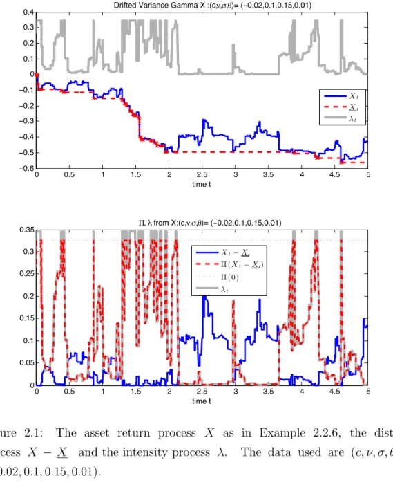
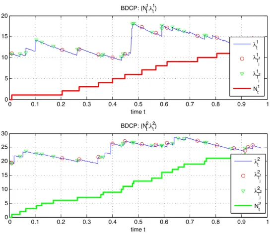
Numerical Illustration We next give a numerical example to illustrate the re-sults. We take the variance gamma process V G(c,ν,σ,θ) in Example 2.2.6. The data used are (c,ν,σ,θ) = (−0.02,0.1,0.15,0.01). Figure 2.1 displays for t ∈ [0,5] a sample path of the asset return process X, the running minimum process X, and the resulting intensity processλ. Figure 2.1 also shows the distance Xt−Xtand its
contributionΠ(Xt−Xt) to the intensity. We can observe the reciprocal relation of
the intensity λt and the distance Xt−Xt, which is consistent with the observation
in the credit market. The upper boundΠ(0) is reached when Xt−Xt = 0, i.e. the
process X reaches a new minimal level, and the intensity λt at that time is above
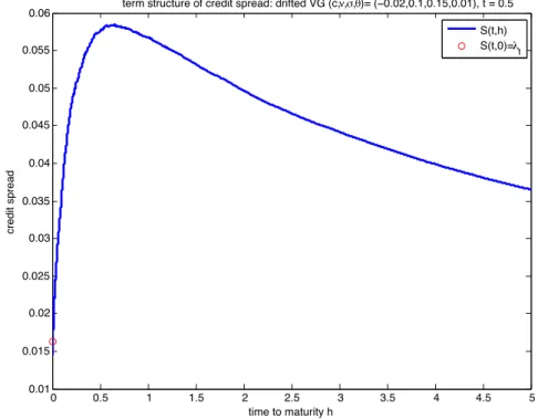
Π(0) by the amount |c| as the drift parameter c < 0. Figure 2.2, using the same sample path of Figure 2.1, shows the term structure of the credit spread h.→S(t, h) at time t= 0.5, starting from S(t,0) =λt.
2.3
Proof of the Main Theorem
The main result Theorem 2.2.2 is proved in four steps, detailed in Subsection 2.3.1 to 2.3.4. Subsection 2.3.1 shows the relation between the likelihood processes (conditional probability process) under different filtrations (Lemma 2.3.2), Subsec-tion 2.3.2 and 2.3.3 establish the existence of the instantaneous likelihood process for a spectrally negative L´evy process with finite variation (Proposition 2.3.8) and for a general L´evy process with finite variation (Proposition 2.3.11) respectively, and Subsection 2.3.4 confirms the indistinguishability of the instantaneous likeli-hood process and the intensity process using Aven’s condition.
2.3.1
Compensators and Likelihood Processes under
Dif-ferent Filtrations
By the Doob-Meyer decomposition, there exists a unique, increasing, G-predictable process A, the G-compensator of N, such that the difference of A and N is a uniformly integrableG-martingale. Moreover, the probabilistic properties of default and stopping time are closely linked to the analytic properties of the compensator. Therefore our objective is to find A.
The conditional survival probability at each time t is given by
Zt:=P(τ > t|Ft) =P(Xt> D|Ft) =eXt,
and let Zt−= lims↑tZs and Z0−= 1.
The following theorem shows the representation of the compensator A under the expanded filtration G.
0 0.5 1 1.5 2 2.5 3 3.5 4 4.5 5 −0.6 −0.5 −0.4 −0.3 −0.2 −0.1 0 0.1 0.2 0.3
0.4 Drifted Variance Gamma X :(c,ν,σ,θ)= (−0.02,0.1,0.15,0.01)
time t Xt Xt λt 0 0.5 1 1.5 2 2.5 3 3.5 4 4.5 5 0 0.05 0.1 0.15 0.2 0.25 0.3 0.35 time t Π, λ from X:(c,ν,σ,θ)= (−0.02,0.1,0.15,0.01) Xt−Xt Π(Xt−Xt) Π( 0) λt
Figure 2.1: The asset return process X as in Example 2.2.6, the distance process X − X and the intensity process λ. The data used are (c,ν,σ,θ) = (−0.02,0.1,0.15,0.01).
Theorem 2.3.1(Jeulin and Yor [43]). Define a nondecreasingF-predictable process
A by At= ) t 0 dKs Zs− ,
0 0.5 1 1.5 2 2.5 3 3.5 4 4.5 5 0.01 0.015 0.02 0.025 0.03 0.035 0.04 0.045 0.05 0.055 0.06 time to maturity h credit spread
term structure of credit spread: drifted VG (c,ν,σ,θ)= (−0.02,0.1,0.15,0.01), t = 0.5 S(t,h) S(t,0)=λt
Figure 2.2: The term structure of credit spread S(t, h): the asset return process X
as in Example 2.2.6 with the data (c,ν,σ,θ) = (−0.02,0.1,0.15,0.01), X−X at
t= 0.5 is 0.0585. 1−Zt =P(τ ≤t|Ft).
Then, the process N−Aτ is a G-martingale, where Aτ = (A
t∧τ)t≥0.
Theorem 2.3.1 shows that one can transform the problem of finding the G -compensator ofN into the problem of finding theF-compensator of Z. As the base filtration F is the natural filtration generated by the asset value process X, all we need to investigate is the path property of X.
If Z is a continuous process, then for any t ≥ 0 we have Kt = −Zt and At =
−ln(Zt) is found explicitly. This is the case discussed in different setups in previous
literature. If Z is discontinuous, then finding K is nontrivial, see [38]. In the following, we aim to find the representation of K.
We first show in the lemma below the pre-limit likelihood processes kh related
Lemma 2.3.2. For any L´evy process X, h >0, define kth := 1 hE[Kt+h−Kt|Ft] and λ h t := 1 hE[Nt+h−Nt|Gt]. Then, kht =eXt1 hE 1 1−e−(y−Xh)+2 333 y=Xt−Xt and λht = 1{τ>t}e−Xtkth. (2.9) Proof. Since Xt+h−Xt = inf u∈[t,t+h]Xu∧Xt−Xt = inf u∈[0,h](Xt+u−Xt)∧(Xt−Xt)−(Xt−Xt) = − . (Xt−Xt)− inf u∈[0,h](Xt+u−Xt) /+ , we have E4eXt+h−eXt|F t 5 = eXtE4eXt+h−Xt −1|F t 5 = eXtE 1 e−((Xt−Xt)−infu∈[0,h](Xt+u−Xt))+ −1|Ft 2 = eXtE 1 e−(y−Xh)+ −12 333 y=Xt−Xt ,
where the last equality comes from the independent and stationary increment prop-erty of the L´evy process X and the adaptedness of X and X to F. Since K is the
F-compensator of 1−Z, the Doob-Meyer decomposition says that
E[Kt+h−Kt|Ft] =−E[Zt+h−Zt|Ft] =−E 4 eXt+h−eXt|F t 5 .
Combining the above gives kh
t in (2.9).
Next, by the optional projection theorem (Theorem 14, Chap.VI, [59] and [34]), we know that if a random variable ξ is nonnegative and integrable, then for each
t≥0, the right continuous version of E[ξ|Gt] is given by
E[ξ|Gt] = 1{τ>t} 1 ZtE 4 ξ1{τ>t}|Ft 5 +ξ1{τ≤t} a.s. (2.10) Therefore, using the tower property of the expectation and the fact that K is
the F-compensator of 1−Z, we have λht = 1 hE[Nt+h−Nt|Gt] = 1{τ>t} 1 h 1 ZtE 4 1{t<τ≤t+h}|Ft 5 = 1{τ>t} 1 h 1 ZtE [Zt−Zt+h|Ft] = 1{τ>t} 1 Zt 1 hE[Kt+h−Kt|Ft]. = 1{τ>t}e−Xtkth. This gives λh t in (2.9).
Remark 2.3.3. Note that ξ1{τ≤t} in (2.10) is Gt measurable. Indeed, since ξ and
τ are random variables on (Ω,G,P), then ξ1{τ≤t} isG-measurable. To show it is Gt
measurable, it is equivalent to show∀b ∈R, B(b) :={ω :ξ(ω)1{τ≤t}(ω)≤b}∈Gt.
Note that B(b)∩{t <τ} = {ξ1{τ≤t} ≤b}∩{t <τ} = ({ξ≤b,τ ≤t}∪{0≤b, t <τ})∩{t <τ} = {0≤b, t <τ} = {b <0}∅+{b ≥0}{t <τ} = {b <0}(∅ ∩{t <τ}) +{b ≥0}(Ω∩{t <τ}).
Since∅,Ω∈Ft for allt≥0, we can take Bt(b) := 1{b<0}∅+ 1{b≥0}Ω∈Ft, such that
B(b)∩{τ > t}=Bt(b)∩{τ > t}.
Therefore, we have B(b)∈Gt.
The next result follows immediately from Lemma 2.3.2.
Corollary 2.3.4. Define ˜ kt := lim h↓0 k h t
and assume it exists for all t a.s., then the instantaneous likelihood process on
{τ > t} is given by ˜ λt:= lim h↓0 λ h t = lim h↓0 1 hP(t <τ ≤t+h|Gt) = e −Xt˜k t.
2.3.2
Spectrally Negative L´
evy Process with Finite
Varia-tion
By (2.9) the existence of the limit processes of kh and λh depends on the path
property of asset value process X and its running minimum process X. In this subsection, let X be a spectrally negative L´evy process with finite variation, we find the limit process using properties of one-sided jump processes. Though the technique in this part can not be extended directly to the more general L´evy pro-cesses of finite variation that contain double-sided jumps in (2.3), the result for these specific processes will play an important role in the next subsection.
The spectrally negative process X has a representation [50, page 56]
Xt=ct−St, (2.11)
where c > 0 and S is a pure jump subordinator with L´evy measure π. (2.11) is a special case of (2.3) with π′ = 0 and c > 0. The L´evy measure of X is πX(dx) =
π(d(−x)) = π((−x,−x+dx]) on R− and if π admits a density ν then π(−dx) =
ν(−x)dx. The following concept is needed in analysing the path properties of X.
Definition 2.3.5 ([50]). Let X be a L´evy process. A point x ∈ R is said to be
irregular for an open or closed set B if Px
*
τB = 0+ = 0, where the stopping time
τB = inf{t >0 :X
t∈B}.
We know ([27, Chapter 9, Proposition 15]) that for X defined in (2.11), 0 is irregular for (−∞,0). Hence, starting at 0, it takes X strictly positive time to reach (−∞,0). If we define T1 := inf{t > 0 : Xt <0}, then P(T1 > 0) = 1. T1 is
the first jump time of X but may not be the first jump time of X. We observe that
X is a pure-jump process as X can only move when S jumps and X cannot jump to a pre-specified level on (−∞,0) as X cannot, see [50, Exercise 5.9]. Hence, the jump size of X has no atoms and is strictly negative. The number of jumps of X
on the interval [0, t], i.e., nt := #{s ∈ (0, t] : Xs = Xs}, is a discrete set and is
a.s. finite. Moreover, we denote the arrival times of nt by (Ti)i≥1, the inter-arrival
times by (δi)i≥1, and the jump sizes by (ξi)i≥1. Then we have the following lemma. Lemma 2.3.6. For X defined in (2.11), X can be written as a renewal-reward process Xt=− nt -i=1 ξi,
where (δi,ξi) are i.i.d. random variables.
Proof. The analysis above shows that X is a non-explosive marked point process
and can be written as Xt = −
,nt
i=1ξi, where −ξi = ∆XTi = XTi −XTi−1 = XTi−XTi−1. (Ti)i are also jump times of L´evy process X and are stopping-times.
We have that (δi,ξi)i are i.i.d. random variables due to the strong Markov property
of X stated in Proposition 2.1.12.
Instead of investigating the exact law of X, we only need to analyse the small-time behaviour of the process, which can be done with the help of the next result, called the Ballot Theorem[11, Proposition 2.7] for drifted subordinators.
Lemma 2.3.7 (Bertoin [11]). Let X be defined in (2.11) and T1 := inf{t > 0 :
Xt<0}. Then, for every t >0, z ≥0, and u <−z,
P(T1 ∈dt, XT1−∈dz,∆XT1 ∈du) = z
ctP(Xt∈dz)π(−du)dt,
where ∆Xt =Xt−Xt− and π is the L´evy measure of S.
Hence the joint distribution of (T1, XT1) is given by
P(T1 ∈dt, XT1 ∈dw) = .) z∈(0,∞) zπ(z+d(−w))P(Xt ∈dz) / 1 ctdt (2.12)
forw≤0. The following is another version of the Ballot theorem:
P(T1 > t, Xt ∈dx) =
x
ctP(Xt∈dx)
for every t >0 andx∈[0,∞). Since Xt=ct−St ≤ct, we have
P(T1 > t) = 1 ct ) ∞ 0 xP(Xt ∈dx) = 1 ct ) ct 0 xP(Xt∈dx) = 1 cE 6 1{0≤Xt≤ct} Xt t 7 .
Note as limt↓0 Stt = 0 a.s., we have for almost all ω, there exists t0(ω), such that for
all t∈[0, t0(ω)],St(ω)≤ct, hence 0≤Xt(ω) =ct−St(ω)≤ct and
lim
t↓0 1{0≤Xt≤ct} = 1 a.s. (2.13)
The dominated convergence theorem leads to lim t↓0 P(T1 > t) = 1 cE 6 lim t↓0 1{0≤Xt≤ct} Xt t 7 = 1 c ·c= 1. (2.14)
Proposition 2.3.8. Let X be defined in (2.11) and let Assumption 2.2.1 be
satis-fied. Then the following limit exists for all t a.s.
˜ kt:= lim h↓0k h t =eXtΠ(Xt−Xt) where kh
t is defined in (2.9) for h >0 andΠ is defined in (2.6). The instantaneous
likelihood process λ˜t defined in Corollary 2.3.4 is given by
˜
λt := lim h↓0 λ
h
t =Π(Xt−Xt).
Proof. Recall that Xt = −,nt
i=1ξi is a renewal-reward process, where the jump
size ξi and inter-arrival times δi are positive random variables for all i, and (δi,ξi)
are i.i.d. random variables.
By (2.14), denote by F the distribution function of δi. Then
lim
t↓0 F(t) = limt↓0 P(T1 ≤t) = 0 =F(0).
Hence, F is right continuous at zero, i.e. F(0) =F(0+) = 0. Define by, for t >0 and y≤0,
Λ0t(y) := 1 tE 1 1−e−(y−Xt)+ 2 Λ1t(y) := 1 tE 1 1{nt=1}(1−e−(ξ1+y) + )2 Λ2t(y) := 1 tE 8 ∞ -k=2 1{nt=k} # 1−e−(!ki=1ξi+y) +$ 9 . We have Λ0t(y) = 1 tE 1 1−e−(y+!nti=1ξi) +2 =Λ1t(y) +Λ2t(y).
We next show that for y≤0, lim t→0Λ 1 t(y) =Π(−y), and limt →0Λ 2 t(y) = 0. (2.15)
Since δ1 and δ2 are independent, also noting (2.12), we have E11{nt=1}(1−e−(ξ1+y) + )2 (2.16) = E11{T1≤t}1{T2−T1>t−T1}(1−e −(ξ1+y)+) 2 = ) t 0 ) ∞ −y ¯ FT1(t−s)(1−e− x−y)P(T1 ∈ds, XT1 ∈d(−x)) = ) t s=0 ) ∞ x=−y ¯ FT1(t−s)(1−e− x−y) .) ∞ z=0 zπ(z+dx)P(Xs ∈dz) / 1 csds = 1 c ) t s=0 ¯ FT1(t−s) ) ∞ z=0 .) ∞ u=0 (1−e−u)π(z−y+du) / zP(Xs ∈dz) s ds = 1 c ) t s=0 ¯ FT1(t−s) .) cs z=0 Π(z−y)zP(Xs ∈dz) s / ds.
The last equality is due to Xs=cs−Ss ≤cs.
Since S is a pure jump subordinator, we have ([50, Lemma 4.11]) limt→0 Stt =
0 a.s., which implies
lim
t→0 Xt
t =c. (2.17)
Using (2.17) and (2.13), the dominated convergence theorem, continuity of Π(·), and X0+ = 0, we obtain lim s↓0 ) cs z=0 zΠ(z−y)P(Xs∈dz) s = lims↓0 E 6 1{0≤Xs≤cs} Xs s Π(Xs−y) 7 = E 6 lim s↓0 1{0≤Xs≤cs} Xs s Π(Xs−y) 7 = cΠ(−y).
Taking the limit in (2.16) gives lim t↓0 Λ 1 t(y) = 1 clims↓0 ) cs z=0 zΠ(z−y)P(Xs∈dz) s =Π(−y).
Here we have used the fact that if g(·) is a nonnegative function and ¯F(0+) = 1, then 1 t ) t 0 ¯ F(t)g(s)ds≤ 1 t ) t 0 ¯ F(t−s)g(s)ds≤ 1 t ) t 0 g(s)ds and lim t→0 1 t ) t 0 ¯ F(t−s)g(s)ds = lim t→0 1 t ) t 0 g(s)ds =g(0+).
We have proved the first limit in (2.15). We next prove the second limit in (2.15). Since Λ0t(0) = 1 tE 4 1−eXt5 ≤ 1 tE 4 1−e−St5 = 1 t * 1−e−Π(0)t+≤Π(0) and 0≤Λ1t(0) ≤Λ0t(0)≤Π(0),
the first limit in (2.15) implies lim t→0Λ 0 t(0) = lim t→0Λ 1 t(0) =Π(0), therefore lim t→0Λ 2 t(0) = 0.
On the other hand, we know 0≤Λ2
t(y)≤Λ2t(0) for all y≤0,
which proves the second limit in (2.15). Hence, Λ0
t(y) = Π(−y) and ˜λt =Λ0t(Xt−
Xt) =Π(Xt−Xt).
Remark 2.3.9. Note that onR+,Π(·) is continuous asπ(dx) is and it is decreasing
with the upper bound Π(0) = −lnE[e−S1] being the Laplace exponent of S from
the L´evy-Khintchine formula. 0 <Π(x)≤Π(0) <(0∞uπ(du)<∞for allx≥0 by Assumption 2.2.1, and therefore Π is bounded on R+.
2.3.3
L´
evy Process with Finite Variation
In this subsection we investigate the limit processes ˜k and ˜λ with X being a L´evy process with finite variation which is a more general class of processes than the last subsection. X then has a representation (2.3)
Xt=ct−St+St′, t≥0
where c ∈ R, S has the L´evy measure π, and we assume Assumption 2.2.1 hold. Note that the path properties and techniques used in Subsection 2.3.2 no longer hold. In (2.3), denote the drift and negative jump components as
Zt(c) :=ct−St.
Lemma 2.3.10. For any c∈R and y≤0 the following limit exists: lim h→0 1 hE 1 1−e−(y−Zh(c))+ 2 = −c1{y=0}1{c<0}+Π(−y), (2.18) where Π is defined in (2.6).
Proof. For c > 0 the limit (2.18) has been proved in the previous subsection. We
now consider the case of c ≤ 0. Note that Zh(c) is decreasing in h and Zh(c) =
Zh(c). We split the proof into two cases.
(i) y= 0: We have lim h→0 1 hE 1 1−e−(y−Zh(c))+ 2 = lim h→0 1 hE 4 1−ech−Sh5 = −c+Π(0).
(ii)y <0: Take the function f(x) := 1−e−(y+x)+
which is bounded, continuous, and vanishes in a neighbourhood of zero: take ϵ<−y, then for any x∈ (0,ϵ), we havef(x) = 0. Hence lim h→0 1 hE 1 1−e−(y−Zh(c))+ 2 = lim h→0 1 hE[f(−Zh(c))] = ) Rf(x)π(dx).
The second equality is due to [60, Corollary 8.9] and π being the L´evy measure of
−Zh(c). Therefore, ) Rf(x)π(dx) = ) ∞ −y (1−e−(y+x))π(dx) = ) ∞ 0 (1−e−u)π(−y+du) =Π(−y), which proves (2.18).
We present the main result in this subsection in the following proposition.
Proposition 2.3.11. Let Xt be defined in (2.3) and let Assumption 2.2.1 be
sat-isfied. Then the following limit exists for all t a.s.
˜ kt := lim h↓0 k h t =eXt * −c1{Xt−Xt=0}1{c<0}+Π(Xt−Xt) + , (2.19) where kh
t is defined in (2.9) for h >0 andΠ is defined in (2.6). The instantaneous
likelihood process λ˜t defined in Corollary 2.3.4 is given by
˜
Proof. The expression of ˜λt in (2.20) is an immediate result of Corollary 2.3.4 and
(2.19). To prove (2.19) we only need to show that for all y≤0, lim h→0 1 hE 1 1−e−(y−Xh)+ 2 =−c1{y=0}1{c<0}+Π(−y). (2.21) Since f(x) = 1−e−(y−x)+
is a decreasing function of x on R− and Xh = ch−
Sh+Sh′ ≥ch−Sh =Zh(c) for all ω and h >0, we have
Xh ≥Zh(c) and 1 hE 1 1−e−(y−Xh)+ 2 ≤ 1 hE 1 1−e−(y−Zh(c))+ 2 .
Using Lemma 2.3.10 we obtain lim sup h→0 1 hE 1 1−e−(y−Xh)+ 2 ≤ −c1{y=0}1{c<0}+Π(−y). (2.22) Take any ϵ>0, on the set {Sh′ ≤ϵh} we have:
Xh =ch−Sh+Sh′ ≤ch−Sh+ϵh=Zh(c+ϵ),
which yields
Xh ≤Zh(c+ϵ) on {Sh′ ≤ϵh}.
Moreover, as Xh ≤0 for all h≥0, we have almost surely,
Xh = 1{S′ h≤ϵh}Xh + 1{S′h>ϵh}Xh ≤1{Sh′≤ϵh}Xh ≤1{Sh′≤ϵh}Zh(c+ϵ). Therefore we have 1 hE 1 1−e−(y−Xh)+ 2 ≥ 1 hE 1 1−e−(y−1{S′h≤ϵh}Zh(c+ϵ))+2 = 1 hE 1 1{S′ h≤ϵh} # 1−e−(y−Zh(c+ϵ))+ $2 = P . Sh′ h ≤ϵ / 1 hE 1 1−e−(y−Zh(c+ϵ)+ 2 .
The last equality is due to the independence of S and S′. Since limh→0
S′ h
h = 0 a.s.,
which implies limh→0P
#S′ h h ≤ϵ $ = 1, we have lim inf h→0 1 hE 1 1−e−(y−Xh)+ 2 ≥ −(c+ϵ)1{y=0}1{c+ϵ<0}+Π(−y).
Letϵ↓0 in the above inequality, we obtain lim inf h→0 1 hE 1 1−e−(y−Xh)+ 2 ≥ −c1{y=0}1{c<0}+Π(−y), and together with (2.22) we proved (2.21).
Remark 2.3.12. Note that if X is a L´evy process with a L´evy measure πX and
f is a bounded continuous function that vanishes in a neighbourhood of zero, then ([60, Corollary 8.9]) lim h↓0 1 hE[f(Xh)] = ) Rf(x)πX(dx). (2.23)
In our case, we aim to compute lim h↓0 1 hE 1 1−e−(y−Xh)+ 2 .
However, we cannot apply (2.23) directly as X is not a L´evy process if X is not a monotone process. Proposition 2.3.11 can be viewed as an extension for function
f(x) = 1−e−(y−x)+
and L´evy process X with finite variation.
2.3.4
Indistinguishability of Likelihood Process and
Inten-sity Process
We have proved the existence of the instantaneous likelihood process ˜λ when X is a L´evy process with finite variation. Heuristically the intensity process λ of the
G-compensator should be equal to ˜λ on the set {τ > t}. However, they are not necessarily the same.
Example 2.3.13 (Guo and Zeng [37]). Define a stopping time τ := inf{t > 0 :
Wt> y} whereW is a Brownian motion and y >0 is a constant. Suppose Fis the
natural filtration of W. We have τ is a F-stopping time and 1 hP(t <τ < t+h|Ft) = 1{τ>t} h ) h 0 |Wt−y| √ 2πt3 e −(Wt−2ty)2dt−→h↓0 0.
That is, ˜λt ≡ 0 for all t ≥ 0. As τ is predictable under F, the compensator of
Nt= 1{τ≤t} is Nt, which indicates the intensity λ does not exist.
Aven’s condition in the next lemma provides a sufficient condition that ensures ˜
Lemma 2.3.14(Aven’s condition [6]). Iflimh→0λht = ˜λt exists andλht is uniformly
bounded for t >0and h >0a.s., then on {τ > t}, Nt−
(t
0 ˜λsds is a G-martingale,
i.e.,(0t˜λsds is the G-compensator of N.
With the help of the results of previous subsections, we can now present the proof of the main theorem.
Proof of Theorem 2.2.2. Recall (2.9) that on {τ > t}

![Figure 5.1: Observation scenario (S1): A sample path of λ k t compared with its unconditional stationary mean and conditional estimate λ k,F t = E[λ kt |σ{N s 1 , N s 2 , s ≤ t }] for k = 1, 2.](https://thumb-us.123doks.com/thumbv2/123dok_us/646349.2577901/111.892.189.708.183.632/figure-observation-scenario-compared-unconditional-stationary-conditional-estimate.webp)