Variable selection via penalized regression and the genetic algorithm using information complexity, with applications for high-dimensional -omics data

(1)

University of Tennessee, Knoxville

Trace: Tennessee Research and Creative

Exchange

Doctoral Dissertations Graduate School

8-2016

Variable selection via penalized regression and the

genetic algorithm using information complexity,

with applications for high-dimensional -omics data

Tyler J. Massaro

University of Tennessee, Knoxville, [email protected]

This Dissertation is brought to you for free and open access by the Graduate School at Trace: Tennessee Research and Creative Exchange. It has been Recommended Citation

Massaro, Tyler J., "Variable selection via penalized regression and the genetic algorithm using information complexity, with applications for high-dimensional -omics data. " PhD diss., University of Tennessee, 2016.

(2)

To the Graduate Council:

I am submitting herewith a dissertation written by Tyler J. Massaro entitled "Variable selection via penalized regression and the genetic algorithm using information complexity, with applications for high-dimensional -omics data." I have examined the final electronic copy of this dissertation for form and content and recommend that it be accepted in partial fulfillment of the requirements for the degree of Doctor of Philosophy, with a major in Mathematics.

Hamparsum Bozdogan, Major Professor We have read this dissertation and recommend its acceptance:

Vasileios Maroulas, Xiaobeng Feng, Haileab Hilafu, Michael Vose

Accepted for the Council: Dixie L. Thompson Vice Provost and Dean of the Graduate School (Original signatures are on file with official student records.)

(3)

Variable selection via penalized

regression and the genetic

algorithm using information

complexity, with applications

for high-dimensional -omics data

A Dissertation Presented for the

Doctor of Philosophy

Degree

The University of Tennessee, Knoxville

Tyler J. Massaro

August 2016

(4)

(5)

DEDICATION

Isaac Newton famously wrote in a letter to Robert Hooke, “If I have seen further, it is by standing on the shoulders of Giants.” If I have seen

anything, it is first and foremost because my parents realized I needed a pair of glasses. Once properly bespectacled, they hoisted me onto their shoulders to get a better view of the wide and confusing world around us. They’ve been supporting me ever since.

I will never be convinced that anyone else has had parents (or even just 2 people) more invested in his or her success than me. I said it to them after my defense, and I will write it here for anyone reading to see: Bill and Terrie Massaro were with me in every equation, every figure, every table, every page of this thing. This is as much their work as it is mine. For this reason a dedication is unnecessary but I dedicate it to both of you anyway.

To my partner in crime and sister, Marina. I will have no greater friend and no more constructive critic. You play each part beautifully, and I needed both this past year. You helped Sarah and I build a bright future for

ourselves, and I will do everything I can to make yours even brighter than it already is.

To Sarah, my girlfriend of 2 years, my personal hair and fashion

authority, she of an endless and tireless patience. You, too, were here with me through all of the late nights, through my doubts and my struggles, seated next to me on the roller coaster ride that this turned into. The ride isn’t over (sorry, did I not mention that before?), but I feel better knowing that you’ve strapped yourself in here with me. And to your family: you guys took me in and embraced me as your own. If it weren’t for my parents and my sister, you cheered harder for me than anyone else has.

(6)

Getting a Ph.D. never has to take a village, but in my case it did. There is a sizable part of Baldwinsville, NY that has waited for this almost as long as I or my parents or my sister have. I could fill a small stadium

(Pelcher-Arcaro?) with people–old friends of mine, friends and co-workers of my parents and sister, family–who have reached out these past few weeks to cheer me on. I dedicate this to all of you, to the BCSFD, and to the OCFIU.

To my school friends back home in Syracuse, in Rochester, in Knoxville, and abroad or elsewhere. You have all been like family; like brothers. It means everything to me that I can laugh or cry; be frustrated or selfish or down or anxious; get excited and all worked up about sports, TV, or movie drama; throw a frisbee, kick a soccer ball, crush a softball or a kickball or a wiffleball or a volleyball; engage in a deep discussion; make art or music; provide video game lessons; have a drink or too many; share a meal; be a friend with all of you.

Finally, to my family. This includes my parents and my sister, but it also includes everyone else. Everyone who is here supporting me, and especially everyone we had to lay to rest along the way. Giants, each of them, hoisting us onto their shoulders.

I’ve been down here in Knoxville, and all of you were back home holding down the fort. That was the hardest part of these past 5 years. I can’t wait to come home and see you again soon.

(7)

ACKNOWLEDGEMENTS

I would like to start by thanking Dr. Bozdogan for his steady guidance throughout the past year and a half. My decision to completely alter the course of my previous dissertation research was an extremely difficult one. If nothing else, the contents of this dissertation are proof that that

decision–reached over many nights of coffee down at Golden Roast–was indisputably the correct one.

This dissertation is not the only piece of evidence. I look also at how well-prepared I feel for life after Knoxville. Dr. B, you have given me a gift, one that has and will continue to open doors for me as I continue growing as a statistical researcher.

To my committee, Dr.’s Maroulas, Feng, Hilafu, and Vose, I also wish to express my most sincere gratitude. At some point in the last year I’ve

brought questions to each of you, and I’ve had each one answered. I honestly couldn’t have asked for anything more though I know I did. Dr. Maroulas, I would like to especially thank you for taking as much time as you did to chat with me, work with me, and help Sarah and I get set up in Durham next year. Your counsel has been equally important to my growth as a researcher.

To the staff in the Mathematics Department and in the BAS

Department–thank you. So much. None of this is actually possible without you. Pam, my days are always brighter when I see that your door is open, although why you have continued to let me into your office is a mystery since 9 times out of 10 it just means more paperwork, emails, or phonecalls for you.

To Dr. Lenhart, who, from the very beginning, was instrumental in bringing me to Knoxville. Between getting me to land on my feet as a graduate student, helping me study abroad 2 (nearly 3) different times in some of the most exotic places on the planet, sharing your knowledge of

(8)

optimal control theory, and teaching me how to effectively function as a member on a research team, I just want to say thank you.

To Dr. Gray: I cannot begin to thank you enough for all of the work you put into writing letters for me last fall, for your constant willingness to answer any questions I send your way, and your genuine interest in seeing me achieve success.

To Dr. Spring: I eagerly look forward to our continued collaboration with one another. The passion that you have for your work is infectious and it is tangible. To you and your family, I want to thank you for helping make my trip to Melbourne a delightful, memorable, and productive one.

To Dr.’s Esham, Haddad, Hartvigsen, Leary, and Spicka, I would like to thank you for being among the first to show me that any of this was possible.

To all of the students that I have had in class, here at UTK and at Geneseo. You make teaching way too much fun.

To so many of my classmates, too many to name here but I will give it my best shot: Eddie, Nate, Ernest, Andrew, Marina, Murat, Ben, Darrin, Kelly, John, Brian, Peter, Will, R´eka, Jason, Steve. I have found our discussions so incredibly beneficial, and, in some cases necessary to the advancement of the research contained here. Your willingness to let me share this research with you or simply listen while I bounced ideas around ended up being a crucial part of the process.

(9)

And I add my own love to the history of people who have loved beautiful things, and looked out for them, and pulled them from the fire, and sought them when they were lost, and tried to preserve them and save them while passing them along literally from hand to hand, singing out brilliantly from the wreck of time to the next generation of lovers, and the next.

(10)

ABSTRACT

This dissertation is a collection of examples, algorithms, and techniques for researchers interested in selecting influential variables from statistical

regression models. Chapters 1, 2, and 3 provide background information that will be used throughout the remaining chapters, on topics including but not limited to information complexity, model selection, covariance estimation, stepwise variable selection, penalized regression, and especially the genetic algorithm (GA) approach to variable subsetting.

In chapter 4, we fully develop the framework for performing GA subset selection in logistic regression models. We present advantages of this

approach against stepwise and elastic net regularized regression in selecting variables from a classical set of ICU data. We further compare these results to an entirely new procedure for variable selection developed explicitly for this dissertation, called the post hoc adjustment of measured effects (PHAME). In chapter 5, we reproduce many of the same results from chapter 4 for the first time in a multinomial logistic regression setting. The utility and convenience of the PHAME procedure is demonstrated on a set of cancer genomic data.

Chapter 6 marks a departure from supervised learning problems as we shift our focus to unsupervised problems involving mixture distributions of count data from epidemiologic fields. We start off by reintroducing Minimum Hellinger Distance estimation alongside model selection techniques as a worthy alternative to the EM algorithm for generating mixtures of Poisson distributions. We also create for the first time a GA that derives mixtures of negative binomial distributions.

The work from chapter 6 is incorporated into chapters 7 and 8, where we conclude the dissertation with a novel analysis of mixtures of count data regression models. We provide algorithms based on single and multi-target genetic algorithms which solve the mixture of penalized count data regression models problem, and we demonstrate the usefulness of this technique on HIV

(11)

count data that were used in a previous study published by Gray, Massaro

et al. (2015) as well as on time-to-event data taken from the cancer genomic data sets from earlier.

(12)

3.4 Genetic algorithm . . . 33 3.4.1 Chromosome . . . 34 3.4.2 Initialization . . . 34 3.4.3 Evolution . . . 35 3.4.4 Convergence . . . 36 3.4.5 Reliability . . . 37 3.5 Multi-objective GA . . . 37 3.5.1 Weighted sum . . . 38 3.5.2 Pareto ranking . . . 38 3.5.3 Our approach . . . 40 3.6 Discussion . . . 40 3.7 Conclusion . . . 41 Bibliography . . . 41

4 Variable selection via penalized logistic regression and the genetic algorithm 46 Abstract . . . 47

4.1.1 Major differences between logistic and ordinary least-squares regression . . . 48

4.1.2 Literature . . . 49

4.2 Derivation of information criteria . . . 51

4.2.1 Model definition . . . 51

4.2.2 Likelihood function . . . 53

4.2.3 Maximum likelihood estimation . . . 54

4.2.4 Information criteria scoring . . . 62

4.3 Post hoc adjustment of measured effects . . . 63

4.4 Example: ICU data . . . 66

4.4.1 Data description . . . 66

4.4.2 Results: full model . . . 70

4.4.3 Stepwise methods . . . 76

4.4.4 Penalized regression . . . 78

(14)

4.4.6 Post hoc adjustment . . . 85

4.4.7 Discussion . . . 88

Bibliography . . . 92

Appendix: Figures . . . 98

5 Variable selection via penalized multinomial logistic regression and the genetic algorithm 104 Abstract . . . 105

5.1.1 Differences between LR and MLR . . . 105

5.1.2 Other types of MLR . . . 106

5.1.3 Literature . . . 107

5.2.1 Model definition . . . 108

5.2.3 Maximum likelihood estimation . . . 109

5.3 Elastic net multinomial logistic regression solver . . . 115

5.4 Example: Persons living with HIV in Tennessee counties . . . 119

5.4.1 Full model . . . 120

5.4.2 LASSO regression . . . 123

5.4.3 Genetic algorithm . . . 124

5.4.4 PHAME subsetting . . . 124

5.4.5 Comparison between penalized regression, GA subset-ting, and PHAME subsetting . . . 126

5.5 Example: TCGA tumor stage data . . . 128

5.5.1 Data description . . . 129

5.5.2 Kruskal-Wallis one-way ANOVA screening . . . 129

5.5.3 Full model . . . 131

5.5.4 Elastic net multinomial logistic regression . . . 132

5.5.5 PHAME subsetting . . . 132

5.5.6 Comparison between penalized multinomial logistic re-gression and PHAME subsetting . . . 133

5.5.7 Functional gene analysis . . . 137

Appendix: Tables . . . 148

6 Mixture distribution analysis for count data using information complexity 163 Abstract . . . 164

(15)

6.1.1 Poisson distribution . . . 165

6.1.2 Negative binomial distribution . . . 166

6.1.3 Mixture modeling . . . 166

6.1.4 Parameter estimation . . . 168

6.2.1 Mixture of Poisson models . . . 171

6.2.2 Mixture of negative binomial models . . . 172

6.3 Bayes error estimation . . . 174

6.4 Experiment: synthetic data for a mixture of 2 Poisson models 176 6.4.1 Comparison between EM and MHD estimation . . . . 177

6.4.2 Accuracy of information criteria . . . 177

6.5 Example: classifying North Carolina counties by SIDS count . 178 6.5.1 Results . . . 179

6.5.2 Comparison with Symons,et al. (1983) results . . . 181

6.6 Example: PLWH counts in southern U.S. counties . . . 182

6.6.1 Results . . . 183

6.7 Discussion . . . 184

7 Variable selection in mixtures of penalized Poisson regression models 200 Abstract . . . 201

7.1.1 Literature . . . 202

7.2.1 Poisson regression mixture model definition . . . 204

7.3 Algorithm for solving the FMPENR problem . . . 212

7.3.1 Initialization . . . 212

7.3.2 Summary of iterative scheme . . . 213

7.4 Example: synthetic data . . . 214

7.4.1 Case: λg = 1,10,25 . . . 214

7.4.2 Case: λg = 10 for g = 1,2,3 . . . 216

7.5 Example: PLWH in West Virginia counties . . . 217

7.5.1 Full model . . . 218

7.5.2 Component selection . . . 219

7.5.3 FMPENR analysis . . . 223

(16)

7.6 Example: Kidney transplant time-to-failure data . . . 231 7.6.1 Full model . . . 232 7.6.2 Component selection . . . 233 7.6.3 FMPENR analysis . . . 234 7.6.4 Genetic algorithm . . . 237 7.7 Discussion . . . 241 7.8 Conclusion . . . 245 Bibliography . . . 246 Appendix: Figures . . . 251

8 Variable selection in mixtures of penalized negative binomial regression models 263 Abstract . . . 264

8.1.1 Literature . . . 264

8.2.1 Negative binomial regression mixture model definition . 267 8.2.2 Likelihood function . . . 268

8.3 Algorithm for solving the FMNBENR problem . . . 276

8.3.1 Initialization . . . 276

8.3.2 Summary of iterative scheme . . . 276

8.4 Example: PLWH in Tennessee counties . . . 277

8.4.1 Full model . . . 279

8.4.2 Negative binomial mixture modeling . . . 280

8.4.4 FMNBENR analysis . . . 282

8.4.5 GA variable selection . . . 285

8.4.6 HIV/AIDS education in Tennessee . . . 288

8.5 Example: PLWH in the U.S. South . . . 291

8.5.1 Full model . . . 291

8.5.4 GA variable selection . . . 294

8.6 Example: TCGA time-to-event data . . . 295

8.6.1 Full model . . . 296

8.6.4 Case: full model . . . 299

8.6.5 Case: G= 3 . . . 300

8.6.6 GA subset selection . . . 303

(17)

8.8 Conclusion . . . 308 Bibliography . . . 309 Appendix: Tables . . . 314 Appendix: Figures . . . 316 Conclusion 328 Vita 329

(18)

LIST OF TABLES

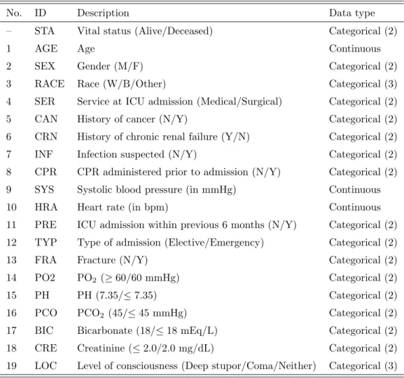
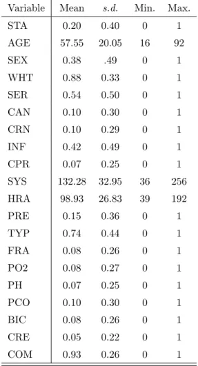
4.1 Description of the variables in the ICU dataset. The outcome is STA. Categorical variables have the number of levels listed in parentheses. . . 68 4.2 Summary statistics for each of the variables considered for the

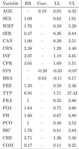
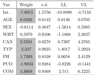
full model. . . 70 4.3 Risk ratios and correlations for each variable with the outcome. 71 4.4 Measured effect of each variable on the outcome, vital status,

as well as the 95% confidence interval bounds. Significant predictors are shaded grey. . . 73 4.5 Hosmer-Lemeshow goodness-of-fit table for the full model.

These results indicate that we do not have significant evidence to reject the null hypothesis that the model fits the data well (χ2 _{= 7}_._80, _df _{= 6,} _P_{-value = 0.25). . . .} ₇₄

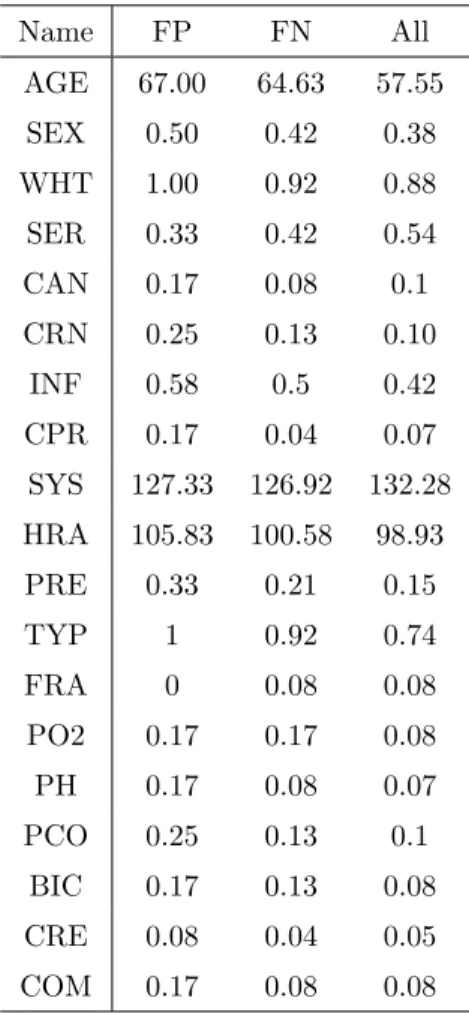
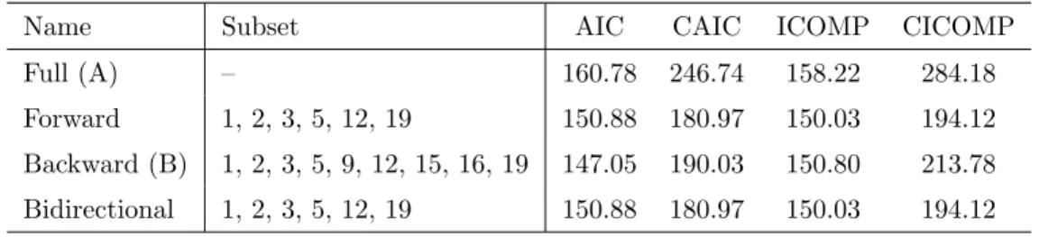
4.6 Average measurement on each variable for observations that are misclassified by the full model as false positives or false negatives. For reference, we include the baseline average across all observations. . . 77 4.7 Information criterion scores for the full model, and the models

chosen using stepwise regression. . . 78 4.8 Measured effect of each predictor on the outcome as well as

the 95% confidence interval bounds using backwards stepwise regression. Significant predictors are shaded in grey. . . 79 4.9 Measured effect of each predictor on the outcome as well as the

95% confidence interval bounds using elastic net regression with

λ1 = 1 andλ2 = 0.5. Significant predictors are shaded in grey. 81

4.10 Measured effect of each predictor on the outcome as well as the 95% confidence interval bounds using elastic net regression with

(19)

4.11 Information criterion scores for the full model, and the models chosen using stepwise regression. . . 83 4.12 CR, MSE, and AUC estimates after 100×10-fold stratified cross

validation using each of the models selected by GA in Table 4.14. 83 4.13 Parameters used to carry out the genetic subsetting. . . 84 4.14 Each of the information criterion scores was used as the

fitness function for 100 trials of a genetic algorithm. The GA parameters are outlined in Table 4.13. Models E and F were selected using AIC as the fitness function. Model G was selected with CAIC; H and I with ICOMP; and, J and K with CICOMP. The number of times each model was selected is italicized next to the subset. . . 85 4.15 CR, MSE, and AUC estimates after 100×10-fold stratified cross

validation using each of the models selected by GA in Table 4.14. 85 4.16 Coefficients from model E in Table 4.14. This model was chosen

by the GA in 95/100 trials when ICOMP was used as the fitness function. Significant predictors are shaded in grey. . . 86 4.17 MATLAB output for the PHAME logistic regression procedure

for variable selection using the ICU data. . . 87 4.18 Subsets chosen by AIC (K), CAIC and CICOMP (L), and

ICOMP (M) from the PHAME analysis. All of the resulting information criteria are shown. Note, Model L is the set of all significant predictors from the original full model. . . 88 4.19 Summary of CR, MSE, and AUC values for Models K through

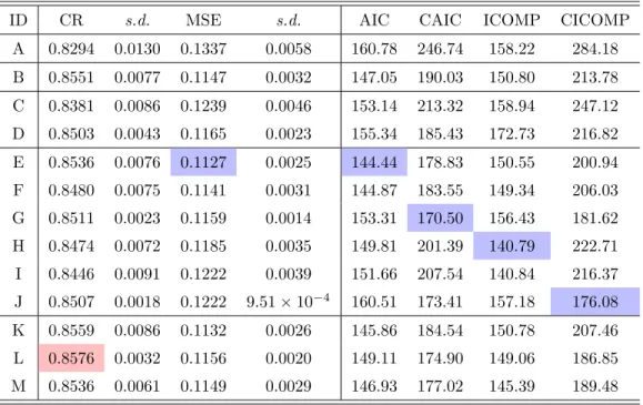
M that were generated during the PHAME analysis. Model L minimized both CAIC and CICOMP with respect to a. . . 88 4.20 Summary of CR, MSE, AIC, CAIC, ICOMP, and CICOMP

values for Models A through M that were generated in this section. The lowest MSE and information criteria scores are shaded in blue; the highest CR is shaded in red. . . 89 5.1 Description of the variables in the PLWH data (Gray et al.

2015). PLWH is the outcome. Categorical variables have the number of levels listed in parentheses. . . 119 5.2 Summary statistics for the Tennessee PLWH data taken from

Gray,Massaro et al. (2015). . . 120 5.3 Summary of PLWH counts by group in the TN data. The

groups were generated using a mixture of Poisson and negative binomial regression models in section 8.4. . . 120

(20)

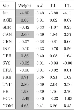
5.4 Weights and confidence intervals for the multinomial logistic regression model fit to the TN PLWH data using class labels from section 8.4. Significant predictors are highlighted in grey. The model is a good fit for these data (χ2 _{= 154}_._98, _df _{= 32,}

P-value <0.001). . . 121 5.5 Weights within each group corresponding to the variable subset

that minimized each of the 4 criteria in a multinomial logistic regression model fit to the TN PLWH data. . . 125 5.6 MATLAB output from PHAME subsetting using the TN

PLWH data. . . 127 5.7 Summary of CR, MSE, AIC, CAIC, ICOMP, and CICOMP

values for Models A through M that were generated in this section. The lowest MSE and information criteria scores are shaded in blue; the highest CR is shaded in red. . . 128 5.8 Number of variables, maximimized log-likelihood values, and

information criteria scores for each of the multinomial logistic regression models discussed in this section fit to the TCGA data. The score minimizers are shaded in blue for each data set. If a model minimized more than one criterion, we denote this with AIC, CAIC, ICOMP, or CICOMP. . . 135 5.9 For each of the multinomial logistic regression models in this

section, we performed 100 simulations of 5-fold cross validation. The observed MSEs, classification rates, and their standard errors are recorded below. The smallest MSEs are shaded in blue, and the highest classification rates are shaded in red. If a model minimized more than one criterion, we denote this with AIC, CAIC, ICOMP, or CICOMP. . . 136 5.10 Average classification rates for 100 simulations of a random

forest, LDA, and K-NN classifiers fit to the different TCGA data sets. Class labels indicated 1 of 4 tumor stages. . . 137 5.11 A list of 250 out of 361 genes selected by the Kruskal-Wallis

one-way ANOVA screen at the 99% confidence level. The full multinomial logistic regression model consists of these 361 genes and an intercept. Table 5.12 contains the remaining genes selected by the screen. . . 148 5.12 A list of 111 out of 361 genes selected by the Kruskal-Wallis

one-way ANOVA screen at the 99% confidence level. The full multinomial logistic regression model consists of these 361 genes and an intercept. Table 5.11 contains the remaining genes selected by the screen. . . 149 6.1 Summary statistics for the North Carolina SIDS data, published

(21)

6.2 Summary statistics for each component in the mixture of 3 Poisson models chosen by the information criteria to model the NC SIDS data. . . 180 6.3 Summary statistics for the PLWH data from Grayet al. (2015). 182 6.4 Summary statistics for each component in the mixture of 3

negative binomial models fit to the PLWH data. . . 184 7.1 Description of the variables in the PLWH data (Gray et al.

2015). PLWH is the outcome. Categorical variables have the number of levels listed in parentheses. . . 217 7.2 Descriptive statistics for the response data in the West Virginia

persons living with HIV data (Grayet al. 2015). . . 218 7.3 Descriptive statistics for the covariate data in the WV PLWH

data (Gray et al. 2015). . . 218 7.4 Weights and 95% confidence intervals from the full model fit

using the West Virginia PLWH data. Significant predictors at the 95% confidence level are highlighted in grey. The maximized log-likelihood is −416.75, and_P[χ2

8 >1950.40]<0.001. . . 219

7.5 Summary statistics for the count data within each of the 3 components from the mixture of Poisson regression models fit to the WV PLWH data. . . 220 7.6 Descriptive statistics for the predictors within each component

of the mixture of 3 Poisson regression models fit to the WV PLWH data. Cells marked in red denote the highest observed average for a component. The average unemployment rate was highest in component 1, although all 3 averages rounded to 0.08. 221 7.7 Weights and confidence intervals for the individual regression

models within each of the G = 3 components. Significant predictors at the 95% confidence level are highlighted in grey. Note that component 3 could only fit a model with 5 predictors since the data here were undersized. . . 222 7.8 Jackknife scores after removing Hardy county from the WV

PLWH data set. . . 223 7.9 Weights for each of the variable subsets chosen by our MOGA

framework using the single Poisson model with λ1 = λ2 = 0.

Models were fit to the WV PLWH data. Red cells indicate risk factors, and blue cells indicate protective factors. . . 227 7.10 We performed MOGA variable subset selection with the finite

mixture of 3 LASSO Poisson regression models fit to the WV PLWH data, withλ1 = 0.0101. The weights are shown for each

component, with risk factors shaded red and protective factors shaded blue. . . 228

(22)

7.11 We used λ1 = 0.0101 to estimate weights in a finite mixture of

3 Poisson LASSO regression models fit to the WV PLWH data. This model clustered the data into 3 groups of data. These 3 groups were fed individually to a Poisson regression model, where we chose variable subsets using a MOGA framework. The weights for each component are shown below with respect to the fitness function used in the MOGA. . . 230 7.12 Description of the covariate data used as predictors in the

kid-ney transplant time-to-failure problem (Le 1997). Categorical-type variables have the number of categories listed in parentheses.231 7.13 Summary statistics for the covariate data in the kidney

trans-plant data set (Le 1997). . . 232 7.14 Summary statistics for the time-to-failure counts in the kidney

transplant data set (Le 1997). . . 232 7.15 Estimated weights and their 95% confidence intervals in the

Poisson regression model fitted to the kidney transplant data. The model is a good fit for the data (χ2 _{= 257}_._88, _df _{= 8,}

P-value <0.001). . . 233 7.16 Summary statistics for the time-to-failure data within each

component in the mixture of 4 Poisson regression models. . . . 234 7.17 Summary statistics for the covariate data within each

compo-nent from the mixture of 4 Poisson regression models fitted to the kidney transplant data. The largest mean value for each variable is highlighted in red. . . 235 7.18 Estimated weights and 95% confidence intervals from each

component in the mixture of 4 Poisson regression models fit to the kidney transplant data. Significant predictors are highlighted in grey. . . 236 7.19 Subsets and associated weights corresponding to the full model

that minimized AIC, CAIC, ICOMP, or CICOMP when fit to the kidney transplant data. . . 238 7.20 Subsets and corresponding weights for the mixture of 4 Poisson

regression models, fitted with identical subsets to the kidney transplant data. We used a MOGA to minimize a convex combination of 90% regression AIC and 10% classification AIC. 240 7.21 Subsets and corresponding weights for the mixture of 4 Poisson

regression models, fitted individually to the kidney transplant data. . . 241 8.1 Summary statistics for the Tennessee PLWH data taken from

(Gray et al. 2015). . . 279 8.2 Descriptive statistics for the dependent variable in the

(23)

8.3 Weights and 95% confidence intervals for the full negative binomial regression model fit to the Tennessee PLWH data set. The log-likelihood is -428.88, leading to χ2₈ = 199.40. The χ2 -statistic has a P-value much smaller than 0.001. Significant variables at the 95% confidence level are highlighted in grey. . 280 8.4 Summary statistics for the count data within each of the 5

components from the mixture of Poisson and negative binomial regression models. . . 282 8.5 Descriptive statistics for the predictors within each component

of the mixture of 5 Poisson and negative binomial regression models. Cells marked in red denote the highest observed average for a component. . . 283 8.6 Estimated weights and their 95% confidence intervals for

pre-dictors within each of 5 components corresponding to either a Poisson or negative binomial regression model. Significant weights at the 95% confidence level are highlighted in grey. . . 284 8.7 Weights corresponding to each variable subset chosen by the

information criteria in the G= 1 case. . . 286 8.8 Weights corresponding to the GA variable subsets within each

of the 5 components based on the information criterion minimized.287 8.9 Summary statistics for the full set of covariates in the U.S. South

PLWH data set (Gray et al. 2015). . . 292 8.10 Weights and their 95% confidence intervals for the full model

using the entire U.S. South data set. Significant variables at the 95% confidence level are highlighted in grey. The maximized log-likelihood is −7564.87, with _P[χ2

8 >1561.14] <0.001. . . . 292

8.11 Correlation coefficients for the 3 racial predictors in the U.S. South PLWH data. . . 294 8.12 Descriptive statistics for time-to-death in the TCGA data

(Kandoth et al. 2013). . . 295 8.13 Descriptive statistics for time-to-death within each component

of the mixture of 3 negative binomial regression models. . . 297 8.14 A breakdown of how often a predictor is significant in the 3

components. More than half of predictors are not significant in any of the components; only 8 appear as significant in all 3. . 298 8.15 A breakdown of how often a predictor is significant in the 3

components after elastic regression with λ1 = 4 and λ2 = 0.1.

More than 90% are not significant in any of the components; only 2 appear as significant in all 3. . . 301

(24)

8.16 Significant gene mutational profiles within each of the 3 compo-nents in the mixture of negative binomial elastic net regression models. The + indicates that the gene mutational profile is positively associated with time-to-death; conversely, − denotes a negative association with time-to-death. Superscripts are included with official gene symbols that appear in 2 or 3 components. . . 302 8.17 Dimension of the variable subset in the models that minimized

each of the 4 information criteria. Additionally, we show the number of significant variables out of the total. . . 304 8.18 Frequency with which predictors appear as significant in each

of the 3 components, in the model which minimized CICOMP. 305 8.19 A list of 250 out of 463 genes selected by the Kruskal-Wallis

one-way ANOVA filter at theα = 0.05 level of confidence. The full model consists of these 463 genes and an intercept. Table 8.20 contains the remaining genes selected by the filter. . . 314 8.20 A list of 213 out of 463 genes selected by the Kruskal-Wallis

one-way ANOVA filter at the α = 0.05 level of confidence for use in the mixture of negative binomial regression models. The full model consists of these 463 genes and an intercept. Table 8.19 contains the remaining genes selected by the filter. . . 315

(25)

LIST OF FIGURES

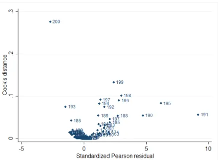
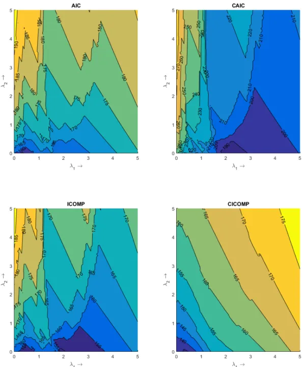
4.1 Cook’s Dvs. the standardized residuals from the full ICU model. 98 4.2 Leveragevs. delta-beta from the full ICU model. . . 98 4.3 Filled contour plots of the cross validation study to determine

λ1 and λ2 for elastic net regression with the ICU data. . . 99

4.4 We fit the ICU data to elastic net regression models for each pair of (λ1, λ2) for λ1, λ2 = 0. . . ,5. We plotted the average

classification rates after 100×10-fold cross validation. . . 100 4.5 We fit the ICU data to elastic net regression models for each

pair of (λ1, λ2) for λ1, λ2 = 0. . . ,5. We plotted the average

MSEs after 100×10-fold cross validation. . . 101 4.6 Trace of the weights as we increase λ1 (λ2 stays fixed at 0) in

the elastic net model. We are able to see how often variables are zeroed out. More persistent variables have been labeled. Data came from the ICU study. . . 102 4.7 Trace of the weights as we increase λ2 (λ1 stays fixed at 0) in

the elastic net model. No variables are zeroed out, however the magnitude of each weight shrinks toward 0. More persistent variables have been labeled. Data came from the ICU study. . 102 4.8 Scores in the top pane, and the trace of PHAME weights for

increasing correlation parameter, a. These models were fit to the ICU data. . . 103 5.1 Information criteria scores in the top pane, and weights in the

bottom panes, corresponding to the multinomial logistic LASSO regression model for increasingL1-penalty. CAIC and CICOMP

(26)

5.2 Weights for increasing correlation parameter,a, during PHAME subsetting of the Tennessee PLWH group data. The black line in each pane denotes where all 4 of the information criteria are minimized. . . 151 5.3 Bar chart for the tumor stages included in our multinomial

logistic regression analysis of the TCGA data. . . 152 5.4 Bar chart for the number of observed mutations occurring in

the TCGA data. Before plotting the log₂(·) of frequencies, we added 1 to each frequency. Hence, true zero counts will appear as zero counts in this chart. . . 152 5.5 Correlation plots for the different subsets of data chosen by the

Kruskal-Wallis one-way ANOVA screen at the 99%, 95%, and 90% confidence levels. . . 153 5.6 Color map of the weights from the full model, which was fit

using 361 screened predictors. . . 154 5.7 We performed elastic net regression, fixing λ2 = 0.1 and

allowing λ1 to vary between 0 and 25. The weights for each

predictor are shown for increasing λ1. The data includes

predictors significant at the 99% confidence level (k = 361). The black bars indicate where the respective criteria are minimized. 155 5.8 We performed elastic net regression, fixing λ2 = 0.1 and

allowing λ1 to vary between 0 and 25. The weights for each

predictor are shown for increasing λ1. The data includes

predictors significant at the 95% confidence level (k = 1292). The black bars indicate where the respective criteria are minimized. . . 156 5.9 Weights from a multinomial logistic regression model fit to

the screened TCGA data (k = 361) for increasing PHAME correlation parameter, a. The black lines denote the subsets where the indicated information criteria were minimized. The right side of the plot has the significant weights; to better see the vanishing weights on the left side of this plot, we restricted significant weights to the opposite side. . . 157 5.10 Weights from a multinomial logistic regression model fit to

the screened TCGA data (k = 1292) for increasing PHAME correlation parameter, a. The black lines denote the subsets where the indicated information criteria were minimized. The right side of the plot has the significant weights; to better see the vanishing weights on the left side of this plot, we restricted significant weights to the opposite side. . . 158

(27)

5.11 Weights from a multinomial logistic regression model fit to the screened TCGA data (k = 2399) for increasing PHAME correlation parameter, a. The black lines denote the subsets where the indicated information criteria were minimized. The right side of the plot has the significant weights; to better see the vanishing weights on the left side of this plot, we restricted significant weights to the opposite side. . . 159 5.12 Glioma pathway, courtesy of DAVID (Jiao et al. 2012). Genes

in this pathway that were significantly associated with tumor stage at the 99% confidence level via Kruskal-Wallis one-way ANOVA are highlighted in red. . . 160 5.13 Endometrial cancer pathway, courtesy of DAVID (Jiao et al.

2012). Genes in this pathway that were significantly associated with tumor stage at the 99% confidence level via Kruskal-Wallis one-way ANOVA are highlighted in red. . . 161 5.14 Prostate cancer pathway, courtesy of DAVID (Jiao et al. 2012).

Genes in this pathway that were significantly associated with tumor stage at the 99% confidence level via Kruskal-Wallis one-way ANOVA are highlighted in red. . . 162 6.1 Graphic showing the pdf of the Poisson mixture modelf(x;π, λ) =

0.4f1(x;λ1 = 7) + 0.6f2(x;λ2 = 20). In red, we see the region

corresponding to the first component, C1, and in blue is the

region corresponding to the second component, C2. When the

two overlap, in violet, observations in C1 are misclassified as

belonging to C2 and vice versa. The area of this region is the

Bayes error, equal here to 0.0342. . . 191 6.2 Along the horizontal axis, we have the difference, δ, in mean

parameters from components in a mixture of 2 Poisson models. For each integer δ along the horizontal axis, we generated 200 samples from a mixture of 2 Poisson models, where (λ1, λ2)

satisfied |λ1 −λ2| = δ. This was repeated 400 times. Along

the vertical axis, the black line is the empirically estimated average Bayes error rate for eachδ. The blue line corresponds to the average misclassification rate for the mixture model whose parameters were estimated using an EM algorithm, and the green line is the misclassification rate for the mixture model fit using MHD estimation. . . 192

(28)

6.3 Refer to Figure 6.2 for an explanation of the experiment. As we increased δ = |λ1 −λ2|, we used the information criteria

AIC, CAIC, and ICOMP to choose the optimal number of components in a mixture model. When δ is large, we see in the top pane that mixture models whose parameters are estimated using an EM algorithm achieve roughly 70% accuracy in identifying G = 2 as the correct number of components. In the bottom pane, we see that MHD estimation leads to mixture models capable of correctly choosing G = 2 in nearly 100% of trials for δ≈15. . . 193 6.4 In the top pane, we see the information criteria scores for

mixture models fitted to the North Carolina SIDS data with up to 5 groups. All but ICOMP select G = 3 as the optimal number of groups. In the bottom pane is the map of North Carolina with the groups labeled. Notice that most of the higher counts correspond to counties with the 11 most populous cities. 194 6.5 The black bars represent the frequencies of observed counts in

the North Carolina SIDS data set. We overlaid the estimated mixture models forG = 1, 2, and 3 components. Note also the maximized log-likelihood values in the legend. We see based on log-likelihood that the 3-component mixture model fits these data best (blue). . . 195 6.6 The top pane shows the information criteria scores following

negative binomial mixture modeling for G = 1, . . . ,8 compo-nents. CICOMP is minimized, and CAIC nearly minimized, for G = 3 components. AIC and ICOMP struggle with issues of overfitting. In the bottom pane, we show the southern U.S. counties colored according to their group. We have additionally provided some major metropolitan areas in each state. . . 196 6.7 The graphic from the bottom pane of Figure 6.6, with names of

cities included. . . 197 6.8 Southern U.S. counties labeled based on the IDs from the

mixture of 7 negative binomial models. . . 198 6.9 Information criteria scores after fitting the PLWH rate data to

mixtures of 1 to 5 negative binomial models. . . 199 7.1 We simulated 3 groups of Poisson regression data. The plot

of these data is shown above, colorized and stylized based on group. The normal variances are σ2

g = 1,2,4 and the Poisson

(29)

7.2 We fitG= 1, . . . ,5 finite mixtures of Poisson regression models to the data from Figure 7.1, with Gopt = 3 chosen as optimal.

The data have been colorized and stylized by the finite mixture model class labels. Data that are filled in are misclassified with respect to the true class labels. The black line through each group is the estimated Poisson regression line fit to each group. 252 7.3 We obtained class labels for the data from Figure 7.1. Based

on these data and the corresponding estimated models, we precisely determined the regions where future observations will be classified by comparing posterior probabilities. . . 253 7.4 Simulation of 3 groups of Poisson regression data, withλg = 10

for g = 1,2,3. We see significant overlap between each group. 254 7.5 Information criteria scores for finite mixtures of G = 1, . . . ,5

Poisson regression models using the WV PLWH data. . . 255 7.6 Map of the West Virginia counties, colorized by component in

the finite mixture of 3 Poisson regression models. Counties with the lowest/highest PLWH counts are in green/red. We have also included the 10 most populous cities in West Virginia. . . 256 7.7 Surface plot of scores for increasingL1- andL2-penalties in the

mixture of 3 Poisson regression models. Increasing λ1 and λ2

leads to poorer models. . . 257 7.8 The upper left pane shows scores for increasing the LASSO

penalty. The remaining 3 panes show what happens to the model weights as λ1 increases. . . 258

7.9 Scores and weights after performing LASSO Poisson regression using the WV PLWH data. . . 259 7.10 Pareto frontier for one iteration of the multi-objective genetic

algorithm. The fitness functions are AIC and AICC. . . 260

7.11 Information criteria scores for mixtures of G= 1, . . . ,5 Poisson regression models fitted to the kidney transplant data from Le (1997). . . 261 7.12 Information criteria scores in the top pane, and corresponding

weights within each of the 4 components, for increasing λ1 in

the mixture of 4 Poisson LASSO regression models fit to the kidney transplant data. It is difficult to tell, but AIC, ICOMP, and CICOMP are minimized for λ1 = 4.08. . . 262

8.1 Information criteria scores for mixtures ofG= 1, . . . ,5 negative binomial mixture models fit to the Tennessee PLWH count data. 316 8.2 Information criteria scores for mixtures of G = 2, . . . ,5 finite

mixtures of mixed Poisson and negative binomial regression models fit to the Tennessee PLWH data set. . . 316

(30)

8.3 Top: Tennessee counties colorized based on membership in 1 of 5 components in the finite mixture of Poisson and negative binomial regression models. Bottom: Tennessee counties colorized based on percentage of the population with less than a high school education. Cross-hatches indicate a county that belongs to component 5 (the highest PLWH counts) and dots indicate a county belongs to component 1 (the lowest PLWH counts). . . 317 8.4 Information criteria scores (top left pane), and weights for

increasing L1-penalty, λ1. The weights for the first component

are in the top right, components 2 and 3 in the middle, and 4 and 5 on the bottom. Notice that the scale of the horizontal axis changes to provide a better understanding of how the weights vanish within each component. . . 318 8.5 Information criteria scores and weights corresponding to

in-creasing L1-penalty in a negative binomial LASSO regression

model for the entire U.S. South PLWH data set. . . 319 8.6 Stem plot for the weights in the negative binomial model

regressing 981 time-to-death data points onto 463 mutation profiles. Only significant predictors have been given nonzero weights. This model exhibited a good fit for the time-to-death data (χ2 = 811.2, df = 464,P-value <0.001). . . 320 8.7 Stem plots and a color map of the weights from the mixture of

3 negative binomial regression models. . . 321 8.8 Scores for mixtures ofG= 1, . . . ,4 negative binomial regression

models fit to the TCGA time-to-death data. CAIC and CICOMP are each minimized forG= 3. . . 322 8.9 Scores in the top pane, and weights in the bottom pane, for

negative binomial elastic net regression using the full TCGA data set. We fixedλ2 = 0.1 and observed the effect of increasing

λ1. CICOMP is minimized for λ1 = 3. . . 323

8.10 Stem plot of the significant weights from the negative binomial elastic net (4, 0.1) regression model fit to the entire TCGA data set. . . 324 8.11 Information criteria scores in the top left pane, and traces of the

weights within each of the G= 3 components in the mixture of negative binomial elastic net regression models (λ2 = 0.1 was

fixed). The intercept is shown to have a weight of approximately 6 in each of the 3 trace panes. Weights that vanished forλ1 ≤10

have been assigned zero-weight to reduce noise. . . 325 8.12 Stem plots and a color map of the weights from the mixture of

(31)

8.13 Stem plots and a color map of the weights from the mixture of 3 negative binomial regression models after performing GA variable subsetting. This model minimized CICOMP. . . 327

(32)

INTRODUCTION

To echo most of what was previously mentioned in the abstract, the first 3 chapters of this dissertation contain background information relevant to the study of the model selection approach to statistical inference and variable subset selection. Chapters 4 and 5 are where we first show our contributions to the statistical literature within the areas of logistic and multinomial logistic regression modeling, respectively. We transition to unsupervised classification problems in chapter 6 as we analyze finite mixtures of

univariate Poisson and negative binomial models. Chapters 7 and 8 continue the theme of unsupervised classification within the context of finite mixtures of regression models. Our hope is that many of the techniques proposed or developed within these last 5 chapters will prove useful for researchers in the fields of epidemiology, public health, and statistical genomics, proteomics, and/or metabolomics.

(33)

CHAPTER

1

MODEL SELECTION VIA INFORMATION

CRITERIA

(34)

Abstract

This chapter serves as an introduction to the topics of information complexity and model selection. We start by briefly presenting an argument in favor of the model selection approach, before describing individual formulas that will be used to compute information criteria scores in this dissertation. When appropriate, we discuss motivating factors behind each of the information criteria, as well as certain tendencies that statistics practitioners can look for when using these criteria in their own research.

1.1

Introduction

The use ofP-values in scientific literature has come under fire recently, with an overwhelming number of researchers seeking alternative means for

evaluating statistical significance. One psychology journal, Basic and Applied Social Psychology, made waves in early 2015 when the editors went so far as to ban the use of P-values in submitted manuscripts.

A problem that many researchers have with P-values goes back to the arbitrary nature with which one assigns significance. For instance, do we use

α= 0.05? 0.01? something else? Is a P-value of 0.02 more significant than a

P-value of 0.03?

Issues with P-values go much deeper than inconsistent significance levels, though. At the heart of the scientific method itself is a necessity to create and assess the validity of hypotheses. As researchers, we create hypotheses based on our intuition about an observable system. By definition, aP-value then represents the probability that we could have obtained a given set of measurements from that system based on the assumption that our hypotheses are true. This definition is fundamentally–albeit only subtly–different from its converse: the probability that our hypotheses are true based on the

(35)

is far too easy and (occasionally) quite lucrative to convolute a narrative that misleads readers into believing something about P-values which is simply untrue.

Later in 2015, FiveThirtyEight, the website run by American statistician Nate Silver, published an articletitled “Science Isn’t Broken,” which profiled recent problems plaguing the peer-review process in scientific literature. An eye-opening feature of this article is its interactive “p-hacking” tool whose instructions are as follows:

You’re a social scientist with a hunch: The U.S. economy is affected by whether Republicans or Democrats are in office. Try to show that a connection exists, using real data going back to 1948. For your results to be publishable in an academic journal, you’ll need to prove that they are “statistically significant” by achieving a low enough p-value.

FiveThirtyEight really hit the nail on the head with this piece: if you go into a scientific study already knowing what it is that you want to show with your data, you’ll be successful if you work hard enough at finding the right

P-value.

Taken with a grain of salt, FiveThirtyEight’s p-hacking tool is not so much an indictment ofP-values as it is an opportunity to reflect on the real issue: evidence-based research is still sometimes more of an art than it is a science. Despite the best intentions of the majority of scientific researchers, it is nonetheless difficult to tease out what it is that data are trying to say.

Model selection exists as an alternative approach for researchers interested in placing less emphasis on P-value-driven statistics. The technique itself

(36)

may be thought of as a lens through which one may establish quantifiable differences between how well distinct statistical models fit the same data set. It is important to point out that model selection is not a replacement for

P-values. Rather, model selection is a tool to be used alongsideP-values when such a multi-faceted approach is possible and appropriate.

The basis for the model selection approach relies on the choice of an appropriate criterion that can be used to compare two or more candidate models. What follows in the remainder of this chapter is an overview of the criteria that will be used throughout this dissertation. We discuss

distinguishing features of each criterion, as well as some of the motivation for preferring one over the other in practice.

1.2

AIC

The first information criterion to see widespread use was the celebrated Akaike Information Criterion (AIC) proposed by Akaike in 1971 and officially published in 1973. AIC has a simple formula:

AIC =−2 log(L(ˆθ)) + 2mk, (1.1)

where L(·) is the likelihood function of our model, ˆθ is the estimated set of parameters that maximizes the log-likelihood and mk is the number of free

parameters in our statistical model. Observe that mk= #(ˆθ); we will

sometimes call this the dimension or order of a candidate model. Also note that when we refer to log(·) we always mean the natural logarithm unless otherwise indicated.

(37)

Each of the terms in the formula for computing AIC represents a specific quantity of information. The first, −2 log(L(ˆθ), tells us about the

“lack-of-fit” of a statistical model. This is not a measure of a statistical model’s deviance from an ideal or “true” model. In the context of model selection, the lack-of-fit only tells us information about how well one model fits data compared to any other model that has been fit using the same data.

The second term, 2mk, is a penalty for overparameterization. In an

abstract sense, overparameterization is problematic since the simplest solution is usually best `a la Occam’s Razor. In a quantifiable sense, we are concerned about excessive parameters in a statistical model because there is a cost to computing them. When we estimate AIC, we explicitly determine that the marginal cost attributable to overparameterization is 2mk, twice the

number of parameters estimated in the model.

It follows naturally that we seek to choose the model with the lowest AIC score. More generally, the model selection approach concerns itself with a search to find a model out of a set of candidate models that best balances the relationship between the lack-of-fit and a corresponding penalty. We will always try to choose a model that minimizes the information criterion with which we are working.

1.3

CAIC and SBC

Bozdogan (1987) derived the consistent form of AIC (CAIC) in response to some researchers calling into question Akaike’s choice of penalty in AIC. The

(38)

equation for computing CAIC is shown below:

CAIC =−2 log(L(ˆθ)) +mk(log(n) + 1). (1.2)

Notice that this equation shares the lack-of-fit component in common with AIC. This is typical of many of the information criteria that have been introduced since AIC; how each of them differ from AIC and each other depends largely on how overparameterization is penalized. With CAIC, we see an overparameterization marginal cost ofmk(log(n) + 1), where n is the

number of observations.

The Schwarz Bayesian Criterion (SBC), also know as the Bayesian

Information Criterion (BIC), has a formula similar to CAIC (Schwarz 1978):

SBC =−2 log(L(ˆθ)) +mklog(n). (1.3)

Schwarz derived the SBC by starting with the assumption that the data distribution comes from the exponential family and then using Bayes’ Theorem. SBC can also be obtained from the Laplace approximation of the posterior distribution of a model. Whereas AIC and CAIC arrive from results related to information theory, the SBC does not. For this reason, we prefer using CAIC over SBC in this dissertation.

1.4

ICOMP and CICOMP

ICOMP, the information-theoretic measure of complexity, is slightly different from AIC and CAIC in that we now introduce a penalty for complexity (Bozdogan 1987, 1988, 1990). Before we explain what this means, observe

(39)

the formula for computing ICOMP:

ICOMP =−2 log(L(ˆθ)) + 2C( ˆF−1). (1.4)

The function C(·) is a real-valued measure of complexity, and ˆF−1 is the estimated inverse Fisher’s information matrix (IFIM) of the model.

We will let C(·) be either theC1(·) or C1F(·) complexity. The formula for

computing C1(·) is as follows: suppose Σ is any square matrix with rank r;

then, C1(Σ) = r 2log tr(Σ) r −1 2log (det(Σ)). (1.5) It is a simple exercise to show that any k-dimensional identity matrix has

C1-complexity equal to 0. Therefore, any deviations of a matrix from the

identity will result in more C1-complexity and a higher penalty. See Van

Emden (1971) for the original derivation of this formula.

The Frobenius-norm characterization of C1(·), called theC1F(·)

complexity, is given by C1F(Σ) = 1 4¯λ2 r X i=1 λi−¯λ 2 , (1.6)

where λi for i= 1, . . . , r refers to an eigenvalue of Σ, and ¯λ is the arithmetic

mean of the spectrum of Σ (Pamukcu 2015).

In addition to ICOMP, we also score the consistent form of ICOMP (CICOMP) (Bozdogan 2010; Pamukcu et al. 2015). The penalty is in place to discourage complexity and promote parsimony just like with ICOMP, but

(40)

we compute this penalty in a slightly different way:

CICOMP =−2 log(L(θb)) +m_k(log(n) + 1) + 2C

ˆ

F−1

= CAIC + 2C F−1. (1.7)

CICOMP penalizes overparameterization more stringently to pick only the simplest models whenever there is nothing to be lost by doing so (Bozdogan 2010).

Consider that the diagonal entries of the IFIM represent the variance of the parameters of our statistical model. Further, off-diagonal elements in the IFIM are covariances between parameters. This means that by including a complexity measure in our scoring of ICOMP, we are penalizing the amount of variability within and among parameters in our model.

Why this is important can be illustrated with the following example. Suppose we are interested in a regression problem in which we use the

variables arm length and leg length to predict weight in male individuals. We can determine the effects associated with arm length and leg length in a regression model, and interpret the results in a straightforward manner. However, a positive correlation exists between arm length and leg length in male individuals. That is, as one’s arm length increases, it is highly likely that his leg length also increases in a predictable way. This phenomenon is known as multicollinearity.

The consequence of multicollinearity is that we expend resources computing excessive information: we may just as easily predict weight in male individuals using only arm length, instead of predicting weight with arm length and leg length. In essence, the complexity measure in ICOMP

(41)

attributes a marginal cost directly to the multicollinear predictors in a statistical model.

1.5

Relationship between

P

-values and AIC

In a regression framework, we can assess the significance of a group of k

variables by computing a χ2_{-statistic based on the deviation of the model}

without those k variables from the full model in which it is nested (Dohoo 2012). Let `(ˆθR) and `(ˆθF) be the maximized log-likelihoods of the reduced

and full models, respectively. Then, the likelihood ratio statistic, λ, is

λ= 2`(ˆθF)−`(ˆθR)

. (1.8)

The significance of the group of k predictors is found by finding the

P-value associated with λ, which isχ2-distributed with k degrees of freedom. If the P-value is smaller than some significance level, e.g.,α = 0.05, we conclude that the group of variables that was removed from the regression model is a significant predictor of the dependent variable.

Suppose now that we compute AIC scores for the full and reduced models. Then, AICR=−2`(ˆθR) + 2mR and AICF =−2`(ˆθF) + 2mF. Define

∆AIC = AICR−AICF. This is precisely

∆AIC = AICR−AICF

=−2`(ˆθR) + 2mR− −2`(ˆθF) + 2mF = 2 `(ˆθF)−`(ˆθR) −2(mF −mR) =λ−2k (1.9)

(42)

Equation (1.9) immediately gives us λ= ∆AIC + 2k. Hence, from equations (1.8) and (1.9), we have the following relationship between the

P-value and ∆AIC:

P =_P[χ2_k >∆AIC + 2k]. (1.10) See Murtaugh (2014) or Bozdogan (1987) for more information on this relationship.

1.6

Discussion

As with any tool, there are numerous advantages and disadvantages to using any one of the different information criteria from this chapter. For example, AIC and CAIC tend to be incredibly easy to estimate. The sole ingredients for computing AIC and CAIC are a statistical likelihood function, the corresponding number of parameters, and the number of measurements in the data set. Generally speaking, the number of parameters is easy to recognize given a likelihood function. Therefore, it is often the case that as long as the log-likelihood function is able to be estimated, AIC and CAIC can be quickly estimated as well.

All of the information criteria from this chapter show remarkable flexibility. In this dissertation, we use AIC, CAIC, and ICOMP in the context of many different types of regression models, including logistic, Poisson, and negative binomial. We also determine the number of

components in mixture model settings, and choose from a set of different distributions the one that provides the best fit to a data set.

The most consistent shortcoming of AIC is that it tends to select models with more predictors than are often necessary. The reason for this relates to

(43)

how Akaike penalized excessive parameterization. It turns out that the amount 2mk is not enough of a penalty when candidate models have many

parameters that need estimating. This is not a reason to abandon AIC; rather, keeping in mind this tendency of AIC often helps to further our understanding of behavior that we see while evaluating different candidate models, especially since we always compare the results of AIC to CAIC and ICOMP.

In practice, there are times when we have data, X, whose Gram matrix

G=XT_X _{is ill-conditioned. This is highly problematic, since it interferes}

with matrix inversions and subsequently our computation of the IFIM for use in estimating ICOMP and CICOMP. One way to avoid this situation is to compute the complexity of the IFIM using C1F(·). The other way involves a

technique known as covariance matrix regularization, which we discuss in the next chapter. Covariance matrix regularization was initially proposed by Bozdogan in 1986 to resolve the improper solutions in factor analytic models with AIC and CAIC.

1.7

Conclusion

In this chapter, we have presented brief background, motivation, and

formulas for various information criteria scores. Of the criteria we described, we will focus almost exclusively on AIC, CAIC, ICOMP, and CICOMP in the chapters to follow.

(44)

BIBLIOGRAPHY

[1] Akaike, H. (1973), “Information theory and an extension of the

maximum likelihood principle,” in Second International Symposium on Information Theory, eds. B. N. Petrox and F. Caski, Budapest, HUN: Akademiai Kiado, pp. 267-281.

[2] Bozdogan, H. (1987), “Model selection and Akaike’s information criterion (AIC): The general theory and its analytical extensions,”

Psychometrika, 52(3), 345-370.

[3] Bozdogan, H. (1988), “ICOMP: A New Model-Selection Criteria,” in Classification and Related Methods of Data Analysis (1998), ed. H. H. Bock, Amsterdam, NED: Elsevier Science Publishers.

[4] Bozdogan, H. (1990), “On the Information-Based Measure of Covariance Complexity and its Application to the Evaluation of Multivariate Linear Models,” Communication in Statistics, Theory and Methods, 19,

(45)

[5] Bozdogan, H. (1994), “Mixture-model cluster analysis using model selection criteria and a new informational measure of complexity,” in Proceedings of the First US/Japan Conference on the Frontiers of Statistical Modeling: An Informational Approach (Vol. 2), ed. H. Bozdogan, Dordrecht, NED: Kluwer Academic Publishers, pp. 69-113. [6] Bozdogan, H. (2000), “Akaike’s information criterion and recent

developments in information complexity,” Journal of Mathematical Psychology, 62-91.

[7] Bozdogan, H. (2010), “A new class of information complexity (ICOMP) criteria with an application to customer profiling and segmentation,”

Istanbul University Journal of the School of Business Administration, 39(2), 370-398.

[8] Dohoo, I., Martin, W., and Stryhn, H. (2012), Methods in epidemiologic research, Charlottetown, PEI, CAN: VER Inc.

[9] Kullback, S. and Leibler, R. A. (1951), “On Information and Sufficiency,” The Annals of Mathematical Statistics, 22(1), 79-86. [10] Murtaugh, P. A. (2014), “In defense of P values,” Ecology, 95(3),

611-617.

[11] Pamukcu, E., Bozdogan, H., and Calik, S. (2015), “A Novel Hybrid Dimension Reduction Technique for Undersized High Dimensional Gene Expression Data Sets Using Information Complexity Criterion for Cancer Classification,” Computational and Mathematical Methods in Medicine, 2015.

(46)

[12] Schwarz, G. (1978), “Estimating the dimension of a model,” The Annals of Statistics, 6(2), 461-464.

[13] Van Emden, M. (1971), An Analysis of Complexity, Amsterdam, NED: Mathematisch Centrum.

(47)

CHAPTER

2

(48)

Abstract

This chapter is dedicated entirely to the concept of covariance estimation. The estimators from this chapter will be especially important when we start considering prolems in later chapters where our data sets are undersampled; the chapter starts by further

expanding on this idea. Without providing much more information in the way of context, we simply use this chapter to collect covariance estimation techniques in one place. All of the estimators in this chapter were tested while performing computational experiments for research related to this dissertation. However, we may have included some estimators despite not specifically mentioning them later, most likely because the one that is referenced will have been the most appropriate for the given problem.

2.1

Introduction

LetX = [x1, . . . , xn]T be our data matrix. For each i= 1, . . . , n, suppose

that xi ∈Rk. That is, eachxi has been measured on k different variables. In

a regression framework, these k variables are predictors. Oftentimes we will add an additional (k+ 1)st variable encoding an intercept.

Suppose n < k. Based on our information, we know that X is a matrix of dimension n×k. Therefore, rank(X)≤min(n, k) =n since n < k is given. It follows that rank(XTX) = rank(X)≤n. ButG=XTX is a k×k matrix, so it must be rank deficient. Thus, when k > n,i.e., when there are more predictors in a data set than observations, the Gram matrix G=XT_X _is

singular. This is hugely problematic, since parameter estimation often relies on obtaining an invertible estimated covariance matrix, which we denote in this chapter as ˆΣ.

This problem is arising more and more often now that -omic data are readily available to researchers. For example, in chapters 4, 5, and 9 we use a data set consisting of n= 3096 cancer patients who were measured for

(49)

mutations in k = 19420 different gene expressions. Such data is often

referred to as flat, owing to the disparity between the number of rows versus columns. Until recently, regression analysis using data of this size was carried out only after the predictors were filtered down to a more manageable size.

One way to counteract the problem of singularities from flat data is by using a technique called matrix regularization. Matrix regularization is a process by which a singular or otherwise ill-conditioned matrix is

transformed so that it becomes invertible. Many regularization formulae exist to perform such a task, which we discuss in the proceeding sections.

2.2

Smoothed covariance estimation

Following the work of Pamukcu et al. (2015), we present the idea behind smooth covariance estimation. Smoothed covariance estimators are a convex combination of the actual estimate of the covariance matrix, ˆΣ, and a

suitably chosen diagonal matrix, ˆD. This is also referred to as “Steinian-type shrinkage” (James and Stein 1961). For some 0< ρ <1, the smoothed estimator of Σ is

ˆ

ΣS = (1−ρ) ˆΣ +ρD.ˆ (2.1)

Our diagonal matrix, ˆD, is the shrinkage target. The naive estimate of ˆD is

ˆ D= tr( ˆΣ) r Ir = 1 r r X i=1 λi ! Ir= ¯λIr, (2.2)

where ˆΣ has rank r, Ir is an r-dimensional identity matrix, and λi for

(50)

entries are the arithmetic mean of the eigenvalues of ˆΣ. The reader is referred to Pamukcu et al. (2015) for more information on estimators of this form.

2.2.1

Convex sum covariance estimator (CSE)

From Chen (1976), we have the convex sum covariance estimator. Let ˆD be as defined previously in equation (2.2); and, for k ≥2 dimensions definem as

0< m < 2 [k(1 +β)−2]

k−β , (2.3)

where we choose β data adaptively:

β= tr ˆ Σ 2 trΣˆ2 . (2.4)

The convex sum covariance estimator is then given by

ˆ ΣCSE = n n+m ˆ Σ + 1− n n+m ˆ D. (2.5)

2.2.2

Bozdogan’s convex sum covariance estimator

(BCSE)

Set α= 1 n−1 k X j=1 Var(xj), (2.6)

where each xj is a column in the data matrixX. That is, we are referring to

(51)

Bozdogan’s convex sum covariance estimator is ˆ ΣBCSE = 1 α ˆ Σ + 1− 1 α D, (2.7)

where D follows from equation (2.2) (Bozdogan 2010).

2.3

Ridge covariance estimation

Ridge covariance estimation involves finding covariance estimators of the form

ˆ

ΣR = ˆΣ +γIr, (2.8)

where r= rank( ˆΣ), Ir is the r-dimensional identity matrix, and γ >0 is a

ridge parameter.

Pamukcu et al. (2015) suggest that this type of covariance estimation is not well-suited to issues involving flat data. Nonetheless, we present some of the work that has been done deriving different ridge parameters, γ. How and why to choose γ remains an open problem, with different researchers offering solutions depending on the problem being addressed.

2.3.1

Maximum likelihood/empirical Bayes

(MLE/EB) covariance estimator

Letr = rank( ˆΣ), andIr be the r-dimensional identity matrix. Then, from

Haff (1980) we have the maximum likelihood/empirical Bayes covariance estimator:

ˆ

ΣM LE/EB = ˆΣ +

r−1

(52)

2.4

Thomaz eigenvalue stabilization

algorithm

From Thomaz’s Ph.D. dissertation (2004), we have the eigenvalue stabilization algorithm. What follows is a heuristic summary of the algorithm.

Start by letting V be the matrix whose columns are the eigenvectors of ˆΣ, and set Λ to be the diagonal matrix whose entries are the corresponding eigenvalues of ˆΣ. Compute ¯λ, the arithmetic mean of the spectrum of ˆΣ.

Next, construct a new diagonal matrix,

Λ∗ = diag max(λ1,¯λ), . . . ,max(λr,λ¯)

, (2.10)

where r= rank( ˆΣ). The stabilized covariance matrix is then defined as

ˆ

ΣST A =VΛ∗V. (2.11)

2.5

Hybridized covariance estimation

The technique of covariance hybridization was proposed by Pamukcuet al.

(2015). The process involves computing ˆΣST A following the algorithm of

Thomaz, but then “hybridizing” the resulting estimator by taking a convex sum of ˆΣST A with another estimator, such as ˆΣCSE or ˆΣBCSE. Pamukcu et al.

(2015) provided the following justification for introducing this new method: “The rationale and mathematical motivation of stabilization plus hybridization are to improve further in a straightforward way the

(53)

smaller and less reliable eigenvalues of the estimated covariance matrix while trying to keep most of its larger eigenvalues

unchange