Demo for Trend Prediction

(1)

Horizon 2020

The word ‘BRAIN’ and neurons, should be

filled with orange. Web safe RGB # F16823

The word ‘fashion’ should be filled with

either white or black

Fashion Brain Logo Branding Sheet

Understanding Europe’s Fashion Data Universe

Demo for Trend Prediction

Deliverable number: D5.5

Version 1.0

(2)

Project Acronym: FashionBrain

Project Full Title: Understanding Europe’s Fashion Data Universe

Call: H2020-ICT-2016-1

Topic: ICT-14-2016-2017, Big Data PPP: Cross-sectorial and cross-lingual data integration and experimentation

Project URL: https://fashionbrain-project.eu Deliverable type Report (R)

Dissemination level Public (PU) Contractual Delivery Date 31 December 2019 Actual Delivery Date 30 December 2019

Number of pages 30, the last one being no. 24 Authors

Ines Arous, Mourad Khayati, Zakhar Tymchenko - UNIFR Ying Zhang, Panagiotis Koutsourakis, Baptiste Kervaut, Martin Kersten - MDBS

Peer review Alessandro Checco - USFD

Alan Akbik - Zalando

Change Log

Version Date Status Partner Remarks

0.1 10/12/2019 Draft UNIFR, MDBS 1.0 30/12/2019 Final UNIFR, MDBS

Deliverable Description

This demo will show how a particular fashion trend (style) is detected on fashion time series over time. The prediction will be implemented as an operator in MonetDB.

(3)

Abstract

Predicting fashion trends is crucial for many fashion companies as it allows them to remain competitive in the market. Several prediction tools have been proposed in this context, but none of them can properly handle the irregularity and the incompleteness in fashion time series. Moreover, existing tools often cannot perform multiple predictions at a time, which helps to simultaneously balance the supply and demand of multiple products. In this deliverable, we present two demo applications in the areas of (fashion) trend detection and prediction.

First, we describe a demo application for trend detection with the combined data processing and text analysis power of a relational database system (i.e. MonetDB) and a machine learning library (i.e. FLAIR) in handling large scale unstructured data (i.e. ∼3TB of 800+ million tweets). This demo is built using the in-database text analysis integration stack reported in deliverable D2.3 “Data Integration Solu-tion”.

Then, we describe a tool to predict the upcoming fashion trends. Our tool overcomes the limitations of existing prediction tools and make it possible to perform multiple predictions on irregular fashion series that contain missing values. This deliverable will benefit from the results obtained in D2.4 and D5.3.

(4)

2.3 Demo implementation . . . 5 2.4 Results . . . 11 3 Trend Prediction 14 3.1 PredTS Algorithm . . . 14 3.1.1 Notations . . . 14 3.1.2 Algorithm . . . 14 3.2 Prediction Tool . . . 16 3.2.1 Implementation . . . 16 3.2.2 Data Description . . . 16 3.2.3 Prediction examples . . . 18 3.2.4 Experiments . . . 20 4 Conclusions 22 Bibliography 23

(5)

List of Figures

2.1 FashionBrain Integrated Architecture (FaBIAM) . . . 4

2.2 Demo workflow . . . 6

2.3 Parallel execution of FLAIR jobs . . . 9

2.4 Number of tweets sent and number of topics discussed . . . 11

2.5 Discussions about “fashion” versus “fashion week” per day . . . 12

2.6 Popularity of fashion brands . . . 12

2.7 Popularity of pop artists . . . 13

3.1 Graphical representation of fashion time series with different time granularities. . . 17

3.2 Prediction of 10 days of sales in a single time series . . . 18

3.3 Prediction of 10 days of sales in multiple time series . . . 19

3.4 Trend Prediction in Weather Time Series . . . 19

3.5 Accuracy comparison of different prediction techniques on fashion data. 20 3.6 Accuracy comparison of different prediction techniques on climate data. 21

List of Tables

2.1 Performance comparison of the renewed JSON support in MonetDB against PostgreSQL and MongoDB. . . 10

3.1 Snapshot from the original data . . . 17

(6)

List of Acronyms and Abbreviations

JSON JavaScript Object Notation

FaBIAM FashionBrain Integrated Architecture

UDFs User Defined Functions

CLOB character large object

NER Named-Entity Recognition

(7)

1 Introduction

1.1 Motivation of the Deliverable

Time series prediction techniques have been extensively investigated in various do-mains including signal processing [14], speech processing [12] and market analy-sis [11, 17, 9]. These techniques have been also used in the fashion industry to predict upcoming trends [15,5,16]. Accurate fashion trends prediction is of a great importance to retailers since it allows them to design their production cycle and remain competitive in the market. Existing trend prediction tools are, however, not convenient for fashion time series which are highly irregular time series [4, 10] and often incomplete.

In this deliverable, we first describe a demo application for (fashion) trend detection with the combined data processing and text analysis power of a relational database system (i.e. MonetDB) and a machine learning library (i.e. FLAIR) in handling large scale unstructured data (i.e.∼3TB of∼800 million tweets). This demo is built using the in-database text analysis integration stack reported in deliverable D2.3 “Data Integration Solution”.

Then, we describe a new online prediction tool that accurately predicts trends in fashion time series. Through our tool, users will observe prediction of multiple time series and will be able to test it on fashion time series with different properties.

1.2 Scope of the Deliverable

This deliverable (D5.5) is part of WP5 in which we perform fashion analysis using time series data. D5.5 extends the work in D5.4, where we classify fashion products based on their fashion features and D5.3, where we predict users’ fashion preferences. In this deliverable, we focus on the detection of (fashion) trends, and the prediction of the fashion time series using their underlying correlations.

For trends detection, D5.5 showcases the in-database machine learning technology introduced in D2.3 on a large Twitter data set. For trends prediction, D5.5 in-troduces a new method to predict the evolution of fashion trends accurately. Also, D5.5 contributes to the research challenges about Analytics for Business Intelligence (i.e., Challenge 9: Time Series Analysis) and the Core Technologies about the ex-ecution layer (i.e., CT2: Infrastructures for scalable cross-domain data integration and management).

For the trends detection demo, we use a Twitter data set that contains 800+ millionThe word ‘BRAIN’ and neurons, should be

The word ‘fashion’ should be filled with either white or black

(8)

1. Introduction 1.2. Scope of the Deliverable

tweets in the period Jul. 01 - Dec. 31, 2014. The information of each tweet is stored in one JavaScript Object Notation (JSON) object. All tweets from the same day are stored in one file. In total, the data set contains 187 JSON files with∼1 billion JSON objects1 _{which take} _∼_{3TB on disk.}

To evaluate our prediction tool, deliverable D5.5 uses the datasets provided by Zalando and described in D2.2. These datasets correspond to the sales in two different regions. Each dataset contains three main columns: the timestamp, the category of items and the corresponding sale of the category with respect to the timestamp. Similarly to the process used in D5.4, these datasets are transformed to time series where each sale’s category represent one time series. The resulting dataset contain 950 time series where the timestamps range from March 2013 to March 2015 with a granularity of 1 day.

1_{Some JSON objects denote the deletion of a tweet. Those were discarded after the preprocessing.}The word ‘BRAIN’ and neurons, should be

(9)

2 Trend Mining

In this section, we describe a demo application we have built for trend detection in Twitter text. This demo is built using the in-database text analysis integration stack reported in deliverable D2.3 “Data Integration Solution”. We leverage the data management and analysis power of the relational database system MonetDB1, and the natural language processing power of the machine learning library FLAIR2 to jointly analyse the topics discussed in a large Twitter data set3 _{to detect trends.} In our analysis, we focus on fashion related trends.

2.1 Background

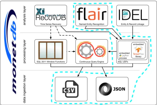
Traditionally, DBMSs only have limited text processing ability, such as substring search and regular expression search; while the machine learning community has much more advanced text analysis tools which are capable of, for instance, under-standing the meaning of the text, such as “wedding dress” vs. “dress for wedding”. To combine the strengths of both worlds, we have presented a FashionBrain In-tegrated Architecture (FaBIAM) in D2.3 “Data Integration Solution”, as shown in Figure 2.1. Through embedded SQL User Defined Functions (UDFs) written in, e.g., Python4_{, we can enrich the analytical features of MonetDB with various advanced} technologies.

In D2.3 “Data Integration Solution” and D2.4 “Time Series Operators for Mon-etDB”, we have demonstrated the main features of all components of FaBIAM us-ing small synthetic data sets. In the context of task T5.4 “Prediction of Fashion Trends”, we have built a demo to showcase the features of the in-database text an-alytics integration stack (as marked by the dashed-box in Figure 2.1) using a large read-world Twitter data set.

This chapter is further divided as follows. First, in Section 2.2, we give a brief description of the data set. Second, in Section 2.3, we describe how the demo is implemented. Finally, in Section 2.4, we present several fashion trends we have detected in this Twitter data set using our integrated MonetDB-FLAIR stack.

1_{https://www.monetdb.org}

2_{https://github.com/zalandoresearch/flair}

3_{We would like to thank Prof. dr. Robert J¨}_{aschke of Humboldt University Berlin & L3S Research}

Center Hannover for providing us this data set. 4

https://www.monetdb.org/blog/embedded-pythonnumpy-monetdbThe word ‘BRAIN’ and neurons, should be

(10)

2. Trend Mining 2.2. Data set description SQL UDFs embedded process embedded library Continuous Query Engine

SQL 2011 Window Functions

Named Entity Recognition

IDEL

Entity & Record Linkage Time Series Recovery

RecovDB

analysis layer

pr

ocessing layer

data ingestion layer

Figure 2.1: the FashionBrain Integrated Architecture (FaBIAM) as presented in D2.3 “Data Integration Solution”. The in-database text analysis integration stack

is marked by the dashed box.

2.2 Data set description

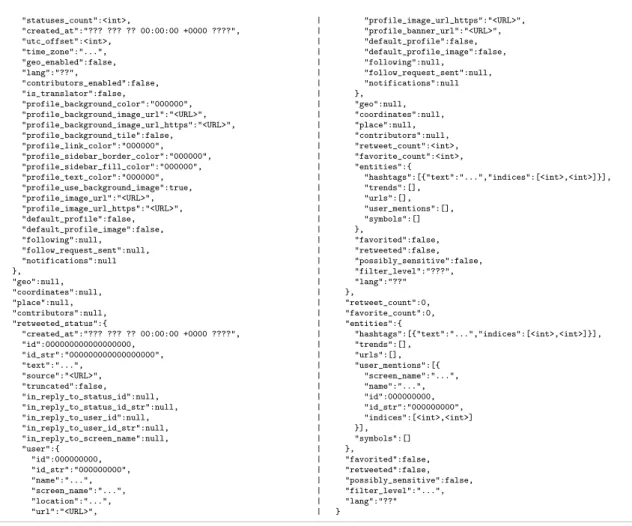
The Twitter data set we have used for this demo contains tweets collected in the period of Jul. 01 – Dec. 31, 2014, which is roughly 1% of all tweets sent in this period. All information of each tweet is stored in one JSON object. The table below shows an anonymised example of one such JSON object containing the information of one tweet:

{ "created_at":"Mon Jul 01 00:00:00 +0000 2014", | "description":"...", "id":000000000000000000, | "protected":false, "id_str":"000000000000000000", | "verified":false, "text":"RT @... : ...", | "followers_count":<int>, "source":"<source URL>", | "friends_count":<int>, "truncated":false, | "listed_count":<int>, "in_reply_to_status_id":null, | "favourites_count":<int>, "in_reply_to_status_id_str":null, | "statuses_count":<int>, "in_reply_to_user_id":null, | "created_at":"??? ??? ?? 00:00:00 +0000 ????", "in_reply_to_user_id_str":null, | "utc_offset":<int>, "in_reply_to_screen_name":null, | "time_zone":"...", "user":{ | "geo_enabled":false, "id":00000000, | "lang":"??", "id_str":"00000000", | "contributors_enabled":false, "name":"...", | "is_translator":false, "screen_name":"...", | "profile_background_color":"000000", "location":"...", | "profile_background_image_url":"<URL>", "url":null, | "profile_background_image_url_https":"<URL>", "description":"...", | "profile_background_tile":false, "protected":false, | "profile_link_color":"000000", "verified":false, | "profile_sidebar_border_color":"000000", "followers_count":<int>, | "profile_sidebar_fill_color":"000000", "friends_count":<int>, | "profile_text_color":"000000", "listed_count":<int>, | "profile_use_background_image":false, "favourites_count":<int>,The word ‘BRAIN’ and neurons, should be | "profile_image_url":"<URL>",

(11)

2. Trend Mining 2.3. Demo implementation "statuses_count":<int>, | "profile_image_url_https":"<URL>", "created_at":"??? ??? ?? 00:00:00 +0000 ????", | "profile_banner_url":"<URL>", "utc_offset":<int>, | "default_profile":false, "time_zone":"...", | "default_profile_image":false, "geo_enabled":false, | "following":null, "lang":"??", | "follow_request_sent":null, "contributors_enabled":false, | "notifications":null "is_translator":false, | }, "profile_background_color":"000000", | "geo":null, "profile_background_image_url":"<URL>", | "coordinates":null, "profile_background_image_url_https":"<URL>", | "place":null, "profile_background_tile":false, | "contributors":null, "profile_link_color":"000000", | "retweet_count":<int>, "profile_sidebar_border_color":"000000", | "favorite_count":<int>, "profile_sidebar_fill_color":"000000", | "entities":{ "profile_text_color":"000000", | "hashtags":[{"text":"...","indices":[<int>,<int>]}], "profile_use_background_image":true, | "trends":[], "profile_image_url":"<URL>", | "urls":[], "profile_image_url_https":"<URL>", | "user_mentions":[], "default_profile":false, | "symbols":[] "default_profile_image":false, | }, "following":null, | "favorited":false, "follow_request_sent":null, | "retweeted":false, "notifications":null | "possibly_sensitive":false, }, | "filter_level":"???", "geo":null, | "lang":"??" "coordinates":null, | }, "place":null, | "retweet_count":0, "contributors":null, | "favorite_count":0, "retweeted_status":{ | "entities":{ "created_at":"??? ??? ?? 00:00:00 +0000 ????", | "hashtags":[{"text":"...","indices":[<int>,<int>]}], "id":000000000000000000, | "trends":[], "id_str":"000000000000000000", | "urls":[], "text":"...", | "user_mentions":[{ "source":"<URL>", | "screen_name":"...", "truncated":false, | "name":"...", "in_reply_to_status_id":null, | "id":000000000, "in_reply_to_status_id_str":null, | "id_str":"000000000", "in_reply_to_user_id":null, | "indices":[<int>,<int>] "in_reply_to_user_id_str":null, | }], "in_reply_to_screen_name":null, | "symbols":[] "user":{ | }, "id":000000000, | "favorited":false, "id_str":"000000000", | "retweeted":false, "name":"...", | "possibly_sensitive":false, "screen_name":"...", | "filter_level":"...", "location":"...", | "lang":"??" "url":"<URL>", | }

In total, there are∼1 billion JSON objects, of which there are 800+ million “actual tweets” (the remaining JSON objects contain information about deleted tweets; they are discarded after the pre-processing).

The tweets of each day are stored in one file. In total, the data set contains 184 JSON files with each file is ∼16GB. The whole data set takes∼3TB on disk.

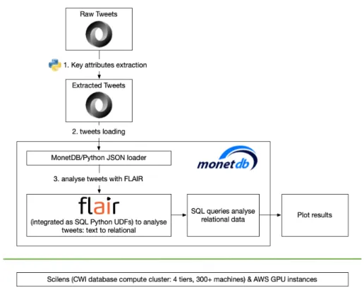
2.3 Demo implementation

Figure 2.2 shows the steps in which this demo has been implemented. For this work, we have used machines both from our Scilens database computing cluster5_{, as well as} several AWS GPU instance6_{. The majority of the work was done using the “Bricks”} machines, each contains an Intel Xeon E5-2650 CPU with 32 cores, 256 GB RAM, 5.4 TB HDD. Some of the Bricks machines also has GPU(s), e.g. “Bricks16” has

5_{https://www.monetdb.org/wiki/Scilens-configuration-standard}

6_{We did not make much use of the AWS instances as we have initially planned, because the GPU}

instances did not give us speedup for the FLAIR jobs and they have too few RAMThe word ‘BRAIN’ and neurons, should be

(12)

2. Trend Mining 2.3. Demo implementation

Figure 2.2: Demo workflow

two nVIDIA GeForce GTX 1080 Ti GPUs with 12 GB on-card Memory7_. Step 1: key attributes extraction

Because we are mainly interested in using FLAIR to analyze the Twitter texts in this demo, and because we do not want to include personal information due to privacy issues, we first extracted a small number of key attributes from the raw Twitter data (as shown above in Section 2.2) for our further analysis:

Tweet ID Date Language Retweet ID Text

Therefore, we have implemented a Python script, which reads the raw Twitter data from each file, extracts the required attributes, and outputs the values of the at-tributes as JSON objects, whose format is supported by the MonetDB/Python JSON loader function8_{, into a file. The extraction takes 6-7 minutes per file, hence,} _∼₂₀ hours in total. The results files are stored under the namestweets {MM} {DD}.json. Initially, we extracted all “actual tweets”. However, when we noticed that running FLAIR takes a long time (more on this in Step 3 below) and many tweets contains languages not supported by FLAIR (e.g. Arabic languages and Asian languages), we

7_{Note that this is not a performance benchmark. Nevertheless, we denote the hardware}

informa-tion and later in this secinforma-tion, some execuinforma-tion times just for the record. 8

https://www.monetdb.org/blog/monetdbpython-loader-functionsThe word ‘BRAIN’ and neurons, should be

(13)

decided to only extract tweets in German, English, Spanish, French, Italian, Dutch and Portuguese. This reduces the amount of tweets used in the FLAIR analysis with ∼50%.

Step 2: tweets loading

In this step, we loaded alltweets {MM} {DD}.jsonfiles into MonetDB and did some post-loading processing of the data.

First, we created a PythonLOADER function:

CREATE LOADER tweets_loader(filename STRING) LANGUAGE PYTHON { import json

f = open(filename) _emit.emit(json.load(f)) f.close()

};

Then the JSON files are loaded one by one:

sql>CREATE TABLE tweets FROM LOADER tweets_loader(‘<path-to>/tweets_json/tweets_07_01.json’) ; operation successful

sql>COPY LOADER INTO tweets FROM tweets_loader(‘<path-to>/tweets_json/tweets_07_02.json’) ; operation successful

...

The “Date” strings from the raw Twitter data are not recognised by MonetDB as timestamps. So, after the initial loading, those “Date” strings are stored in a character large object (CLOB) column, which occurs more disk storage and is less efficient in query processing than when the values are stored as binary timestamps. Therefore, as a final step in data loading, we cast the “Date” strings into timestamps:

ALTER TABLE tweets ADD COLUMN "TimeStamp" TIMESTAMP;

UPDATE tweets SET "TimeStamp" = STR_TO_TIMESTAMP("Date", ’%a %b %d %H:%M:%S +0000 %Y’); ALTER TABLE tweets DROP COLUMN "Date";

On average, loading onetweets {MM} {DD}.jsonfile takes∼25 seconds. Converting the “Date” strings took∼17 minutes. In total, this step took ∼1.5 hour. The final result of this step is a table called “tweets” with ∼400 million tuples table with a disk size of ∼68 GB:

sql>\d tweets

CREATE TABLE "sys"."tweets" ( "Tweet_ID" BIGINT,

"Language" CHARACTER LARGE OBJECT, "Retweet_ID" CHARACTER LARGE OBJECT, "Text" CHARACTER LARGE OBJECT, "TimeStamp" TIMESTAMP

);

sql>SELECT COUNT(*) FROM tweets ; +---+

| L2 |

+===========+ | 404578963 |The word ‘BRAIN’ and neurons, should be

(14)

+---+ 1 tuple

sql>SELECT (SUM("count" * typewidth) + SUM(heapsize))/1024/1024/1024 more>FROM sys.storage() WHERE table = ’tweets’;

+---+ | L5 | +======+ | 68 | +---+ 1 tuple

Step 3: Analyse tweets with FLAIR

Finally, we use FLAIR9 to process the tweet texts, i.e. extract the topics discussed in them. As shown in Figure 2.1, FLAIR was integrated into MonetDB as embed-ded SQL Python UDFs10_{, which was described in detail in D2.3 “Data Integration} Solution”.

We have experienced with various FLAIR models. First, we trained our own models with the help of the Flair tutorials11_. _{We trained a Named-Entity Recognition} (NER) model and a multilingual Part-of-Speech (POS) model. The accuracy of the results were low, because tweets only contain short texts and are extremely noisy with a lot of grammatical errors and shorthands. Then, we used two models provided by Flair: a multilingual NER model and a multilingual POS model, which gave us better results. In particular, the pre-trained POS-multi model was quite good in tagging of nouns and proper nouns.

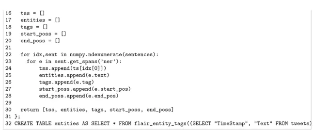
The code snippet below shows one such SQL Python UDFs, which uses the NER model (line 11 - 14) on the inputs STRING. It returns theentitiesfound by FLAIR together with the timestamp associated with the input string and some auxiliary information of this entity (line 30). Finally, we apply this function on the text from the tweets tableand store the results in a new table entities(line 32).

1 CREATE FUNCTION flair_entity_tags (ts TIMESTAMP, s STRING)

2 RETURNS TABLE(ts TIMESTAMP, entity STRING, tag STRING, start_pos INT, end_pos INT) 3 LANGUAGE python

4 {

5 from flair.data import Sentence

6 from flair.models import SequenceTagger 7 import numpy

8

9 # Make sentence objects from the input strings

10 sentences = [Sentence(sent, use_tokenizer=True) for sent in s] 11 # load the NER tagger

12 tagger = SequenceTagger.load(’ner’) 13 # run NER over sentences

14 tagger.predict(sentences) 15

9_{A. Akbik, D. Blythe and R. Vollgraf.} _{Contextual String Embeddings for Sequence}

Label-ing, in Proceedings of the 27th International Conference on Computational Linguistics, pages 1638–1649, August, 2018. Santa Fe, New Mexico, USA.

10_{https://www.monetdb.org/blog/embedded-pythonnumpy-monetdb} 11

https://github.com/zalandoresearch/flairThe word ‘BRAIN’ and neurons, should be

(15)

2. Trend Mining 2.3. Demo implementation 16 tss = [] 17 entities = [] 18 tags = [] 19 start_poss = [] 20 end_poss = [] 21

22 for idx,sent in numpy.ndenumerate(sentences): 23 for e in sent.get_spans(’ner’): 24 tss.append(ts[idx[0]]) 25 entities.append(e.text) 26 tags.append(e.tag) 27 start_poss.append(e.start_pos) 28 end_poss.append(e.end_pos) 29

30 return [tss, entities, tags, start_poss, end_poss] 31 };

32 CREATE TABLE entities AS SELECT * FROM flair_entity_tags((SELECT "TimeStamp", "Text" FROM tweets));

Even though we have worked with colleagues from Zalando research to speed up FLAIR, applying the FLAIR models on this amount of tweets sequentially is still a very time consuming task which can take weeks. Fortunately, multiple Bricks machines have GPUs12. So, eventually, we decided to divide the tweets table into several smaller pieces and run multiple FLAIR UDFs in parallel, as shown in Fig-ure 2.3. We grabbed all Bricks machines that were still available in August 2019 with three of them having 2 GPUs and one having 1 GPU. On each GPU, we could run 2 FLAIR functions. In this way, we were able to speed up the FLAIR execution time with a factor of 14.

By using the FLAIR models, we identified in total∼1.7 billion topics discussed in the tweets of this Twitter data set. All topics are united into a view called all topics

that only contains the triple (dte, hr, topic)to denote the date, hour-of-day of a topic.

2

How to speed up 14 times

bricks bricks bricks bricks

GPU0 GPU1 GPU0 GPU1 GPU0 GPU1 GPU0

Figure 2.3: Parallel execution of FLAIR jobs

Renewed JSON support

The Python script in Step 1 was needed, because at the time when this project was conducted (i.e. summer 2019), MonetDB did not support the loading of the Twitter data in its raw JSON format. After the summer project, we started a new project to renovate MonetDB’s JSON support. At the time of this writing (i.e. end of Nov 2019), MonetDB is able to directly load the raw Twitter JSON data.

12

https://www.monetdb.org/wiki/BricksThe word ‘BRAIN’ and neurons, should be

(16)

MonetDB PostgreSQL PostgreSQL PostgreSQL MongoDB Data set Operation (hg: 08004c77) (11.5 json) (11.5 jsonb) (12.0 jsonb) (4.2.1) 200K JSON obj. data loading 5.65 12.11 18.15 18.40 26.82 (∼570MB) JSON filter 1.26 1.54 0.52 0.51 1.96 2M JSON obj. data loading 53.55 127.49 190.13 190.10 279.89 (∼5.8GB) JSON filter 3.01 16.11 5.24 5.07 18.44

Table 2.1: Performance comparison of the renewed JSON support in MonetDB against PostgreSQL and MongoDB.

Table 2.1 shows some preliminary performance comparisons of the renewed Mon-etDB JSON support (Mercurial commit number 08004c77) against that of Post-greSQL and MongoDB. We used files from the raw Twitter data (an example of a raw JSON object was shown in Section 2.2): one data set contains 200,000 JSON objects; the other data set contains 2 million JSON objects. PostgreSQL can store JSON objects as both strings (i.e. “PostgreSQL 11.5 json”) and as binary data (i.e. “PostgreSQL 11.5 jsonb” and “PostgreSQL 12.0 jsonb”); while MonetDB and MongoDB only store JSON objects as strings. The execution times are averages of 5 runs.

First, we load the JSON files. The execution times are shown in the “data loading” rows in Table 2.1. For both data sets, MonetDB is the fastest system in loading those files. Then, we run a simple filter query to compute the number of real tweets

(i.e. excluding the JSON objects denoting deleted tweets) in the data sets, using the following queries:

-- MonetDB and PostgreSQL SQL query:

SELECT count(*) FROM tweet_data WHERE json.length(json.filter(j, ’$.created_at’)) > 0; -- MongoDB query

db.tweets.find({created_at: {$exists: true}}).count()

For the 200K data set, PostgreSQL (12.0 jsonb) was the fastest; while MonetDB is the fastest for the 2M data set.

When we examine the execution times per column, we can observe that the data loading times of MonetDB and PostgreSQL (11.5 json) scales linearly with growing data size; while the scalability of the other three systems goes towards superlinear. Concerning the filter query, only MonetDB scales sublinearly, the other four systems all scale linearly.

This work is available in the “json” branch13 _{of the MonetDB primary code} repos-itory. We expect to be able to merge this branch into the MonetDB main source code in 2020 for its release in an official MonetDB version.

13_{https://dev.monetdb.org/hg/MonetDB/shortlog/json}The word ‘BRAIN’ and neurons, should be

(17)

2. Trend Mining 2.4. Results

2.4 Results

With the query processing power of an analytical DBMS and the text analysis power of a multilingual machine learning library, we can gain a lot of information from this Twitter data set. Below, we limit the presented results to several fashion related topics without involving any personal information (of Twitter users).

(a) per day (b) per hour-of-day

Figure 2.4: Number of tweets sent and number of topics discussed

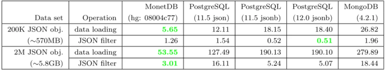
Trend 1: how active are we on Twitter?

Figure 2.4(a) and Figure 2.4(b) show the number of tweets sent and number of topics discussed per day or per hour-of-day, respectively.

The amount of activities on Twitter is more or less stable in this period. The spike on November 9th is possibly caused by several popular events happening at the same time, e.g. some news about Justin Bieber and the plethora of fans campaigning to get the girl group Fifth Harmony the top prize in the 2014 MTV European Music Awards (see also discussion below about Figure 2.7(a) and Figure 2.7(b)). Unfortunately, we cannot find any good explanation for the negative spike in December 2014. Figure 2.4(b) shows that Twitter users are most active from 5 o’clock in the afternoon until 3 o’clock in the morning, and lest active earlier in the morning. This is as what we would expect.

Trend 2: how often do we discuss about fashion?

Figure 2.5 shows that the interest in fashion among the Twitter users is fairly stable over time. Some of the discussions about fashion is devoted to discussing the fashion week, a fashion event organised several times per year in different locations for a whole week. Throughout the year, there is a small amount of tweets about fashion week. However, during the week of an event, this topic obvious attracts more atten-tion, such as shown by the peak in September 2014, which was when the New York Fashion Week was hold.

Trend 3: which brand should I buy to be more trendy?The word ‘BRAIN’ and neurons, should be

(18)

Figure 2.5: Discussions about “fashion” versus “fashion week” per day

(a) Luxury brands (b) Sport brands

Figure 2.6: Popularity of fashion brands

Figure 2.6(a) and Figure 2.6(b) show the popularities of several luxury fashion brands and sport brands, respectively.

According to this data set, Gucci is far more popular than Prada and Burberry. Also, the popularity of the three brands barely overlaps. The amount of interest in Gucci fluctuates considerably over time, while the interests in Prada and Burberry are fairly stable. Spikes in the graph, e.g. those of Prada and Burberry, are generally caused by marketing events. For instance, on Sep. 15th, it was the Full Burberry Prorsum Womenswear S/S15 Show; while on Nov. 19th, the Pradasphere exhibition started in HongKong.

Figure 2.6(b) shows that Nike is generally more popular than Adidas. However, with some strong market, Adidas some times attracts more attention than Nike. For instance, on Jul. 13th, Adidas release the adiZero Prime Boost in the US; andThe word ‘BRAIN’ and neurons, should be

(19)

on Dec. 30th, Adidas released the T-MAC 3 “Chinese New Year”.

(a) Female artists (b) Male artists

Figure 2.7: Popularity of pop artists

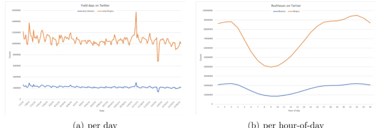
Trend 4: who might have the biggest influence?

By studying the popularity, we can get an idea of how much impact a famous person can have when they do something (i.e. find influencers). Figure 2.7(a) and Figure 2.7(a) show the popularity of several female and male music artists, respectively. From these graphs, we can observe several things. First, the amount of interest the female artists attract was largely affected by famous music event. In Figure 2.7(a), the peak in July - August goes with the 2014 MTV video music awards; while the peak in November goes with the 2014 American music awards. However, according to Figure 2.7(b), the interests in male artists do not show such clear correlation (or maybe they are a bit overshadowed by the news around Justin Bieber).

Second, we already know that Beyonce has not been very active in the recent years, so the social media seems to be a bit quiet around her. However, one live performance of her at the 2014 MTV Video Music Awards on Aug. 25th drove her popularity right through the platform formed by Lady Gaga. Clearly, Beyonce still has a lot of fans. From this, we can probably conclude that as an artist/influencer, Beyonce is a hibernating giant. Once she is back to action, we can expect huge impact from her.

Finally, by comparing the scale of the y-axis of both figures, one can see that the male artists attract by far more attention from the Twitter users than the female artists. This is probably because there is a huge amount of teenage girls on Twitter, which drives the popularities of teenage artists and bands. The huge spike in Justin Bieber’s graph was probably caused by that on November 8th, several pictures of Justin Bieber and Hailey Baldwin were put online.

(20)

3 Trend Prediction

In this section, we describe our online trend prediction tool for time series data. We first describe the algorithm we use for prediction. We show how to leverage the efficiency of the Centroid Decomposition technique [1, 8] to decompose time series and perform accurate prediction. Then, we describe our graphical prediction tool that relies on the data management and analysis power of the relational database system MonetDB1_.

3.1 PredTS Algorithm

3.1.1 Notations

A time series X = {(t1, v1), . . . ,(tn, vn)} is an ordered set of n temporal values vi that are ordered according to their timestampsti. In the rest of the report, we omit the timestamps, since they are ordered. We write X = [X1|. . .|Xm] (or Xn×m) to denote an n×m matrix having m time series Xj as columns and n values for each time series as rows.

3.1.2 Algorithm

Our proposed technique is based on the observation that time series are usually correlated with each other. These correlations can be accurately captured using the Centroid Decomposition (CD) technique (see Deliverable D5.4). In particular, we use CD to find the k dimensions that best explain/summarize the main trends in the collection. For prediction we use an auto-regression (AR) model of orderpthat learns auto-regressive coefficientsαj from previous data and estimates the upcoming values as follows:

ˆ

xt+1 =α1×xt−1+α2×xt−2+. . .+αp×xt−p

where t is the time point of the latest known value and p is the order of the auto-regressive model.

Our technique allows any prediction algorithm to take advantage of the dimensions extraction of the time series collection. It takes a set of m correlated co-evolving series and extracts the principal latent dimensions that best represent the time series.

1

https://www.monetdb.orgThe word ‘BRAIN’ and neurons, should be

(21)

3. Trend Prediction 3.1. PredTS Algorithm

The key components are extracted independently for each time series allowing to predict multiple series at a time.

Algorithm 1 outlines the prediction procedure. First, we decompose a matrix X

of all time series using CD to extract the main components. Each component Li resulting from the decomposition is treated as a uni-variate time series. Then, an auto-regressive model is applied independently for the de-trended component ˆLi and the trend T. The model returns an order p for ˆLi and p0 for T respectively and their coefficients. This allows to perform independent predictions forw points into the future of both parts using auto-regressive weighted sum (where weights are α1, α2, . . . αp and α01, α

0

2, . . . αp0 respectively). When the component prediction

terminates, we re-integrate the trend back into the component ˆLi by adding T to it. Finally, we use the r weights from CD to compute a weighted average of the components ˆLi, and to predict a subset of time series.

Algorithm 1: PredTS(X, P, w)

Input : X: matrix of all time series;

P: set of indices of time series to predict;

w: prediction window size

Output:a set of predicted time series

1 L,R:= CD(X,n,m) ; 2 i:= 1 ;

3 foreachTime series component L_i ∈L do 4 T := SmoothTrend(Li) ;

5 Lˆi:=Li−T ; . Trend removal

. Learning auto-regressive parameters

6 {p,α1,α2 . . .αp} := AR( ˆLi) ; 7 {p0,α0₁,α0₂ . . .α0_p0} := AR(T) ; . Component derivation 8 j :=n+ 1 ; 9 repeat 10 ˆli,j :=Pp_k=1αk×ˆli,j−k ; 11 tj :=Pp 0 k=1α 0 k×tj−k ; 12 j :=j+ 1 ; 13 until j=n+w; 14 Lˆi:= ˆLi+T ; . Trend reintegration

. Time series prediction

15 foreachp∈P do

16 Xˆp :=Pm_i=1Lˆi×ri,p ;

17 return{Xˆ_p₁, . . . , ˆX_p_q} ;

(22)

3. Trend Prediction 3.2. Prediction Tool

3.2 Prediction Tool

3.2.1 Implementation

Our online trend prediction tool2 is a client-server application. The client-side is implemented using JavaScript, jQuery, Highcharts (a JavaScript library for charts) and HTML/CSS. The server-side uses MonetDB database and PHP for preprocess-ing the data. Internally, MonetDB stores the data of each SQL column as a spreprocess-ingle C array.

CREATE TABLE tss(ts timestamp, v1 float, .., vn float); CREATE FUNCTION precict(ts timestamp, v1 float, .., vn float)

RETURNS TABLE (ts timestamp, f1 float, .., fn float) ...; SELECT * FROM predict((SELECT ts, v1, v3, v7 FROM tss

WHERE ts BETWEEN TS MIN AND TS MAX));

The SQL queries above show a skeleton of the implementation. First, we store all time series of one dataset in a single table containing one timestamp column and a number of value columns to hold the values of the time series (after some prepro-cessing to align the timestamps). Then, we implementedPredTS (see Algorithm 1) and its auxiliary functions as native SQL UDFs in MonetDB. The table returning function predict is a wrapper for predTS. It takes one column of timestamps and multiple columns of time series values containing NULLs for the values to predict as its inputs, and passes the value columns to PredTS for prediction. The predicted time series are returned together with the original timestamps in a single table. Fi-nally, we use predict in a SELECT query to predict the values of three time series within a given time period.

3.2.2 Data Description

As fashion data, we use the dataset provided by Zalando. For each category in the Zalando taxonomy3, we have the amount and number of items sold from March 2013 until March 2015. A snapshot of the data is shown in Table 3.1. The first three columns describe the path in the Zalando taxonomy. The fourth column describes the season to which the item belongs: FS (Fr¨uhling Sommer) means “Spring Sum-mer”, HW (Herbst Winter) means “Autumn Winter” and NO means “No season”. We map the original data into time series representation. We define each category as a separate time series and the granularity of each time series as 24 hours. We obtain 960 time series each of length 730. A snapshot of the resulting time series is shown in Table 3.2.

2_{The tool is accessible through our Revival interface:} _{revival.exascale.info/prediction/}

datasets.php

3_{Our fashion taxonomy can be visualized through:} _{https://fashionbrain-project.eu/}

fashion-taxonomy/The word ‘BRAIN’ and neurons, should be

(23)

date level 1 level 2 level 3 season gross amount no items 2013-03-01 0.0 0.0 0.0 FS 2.068 1.82 2013-03-01 0.0 0.0 0.0 HW 1.535 1.66 2013-03-01 0.0 0.0 0.0 NO 0.769 1.80 2013-03-01 0.0 0.0 1.0 FS 1.130 1.32 2013-03-01 0.0 0.0 1.0 HW 3.084 5.47 2013-03-01 0.0 0.0 1.0 NO 0.264 0.54 2013-03-01 0.0 0.0 2.0 FS 0.210 0.27 2013-03-01 0.0 0.0 2.0 HW 1.639 2.62

Table 3.1: Snapshot from the original data

date no items 0.0,0.0,0.0,FS no items 0.0,0.0,0.0,HW no items 0.0,0.0,0.0,NO 3/1/13 1.82 1.66 1.80 3/2/13 2.61 1.75 2.81 3/3/13 3.76 1.22 2.96 3/4/13 3.26 2.19 2.10 3/5/13 3.17 1.62 2.07 3/6/13 3.53 1.37 3.58 3/7/13 2.71 2.04 1.91 3/8/13 2.54 1.75 1.26 3/9/13 3.52 2.06 2.05

Table 3.2: Snapshot from the obtained time series

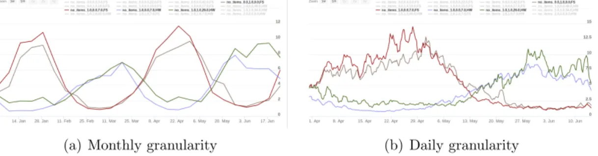
In Figure 3.1 we show four different fashion time series obtained by the aforemen-tioned data mapping. Our tool allows to visualize the series with different time granularities, e.g., day, month and year.

(a) Monthly granularity (b) Daily granularity

Figure 3.1: Graphical representation of fashion time series with different time granularities.

(24)

3.2.3 Prediction examples

In this section, we describe some trend prediction queries. We first show the results of sample queries on fashion time series. Then, we show the results on longer non-fashion related series that exhibit similar properties as the non-fashion dataset.

Prediction 1: Predict 10 days of sales.

Figure 3.2(a) shows the trend prediction of 10 days sales in one fashion time series. The Zalando dataset shows a global monotonic increase of sales during the month of February with larger sales increase which occur during Feb 16-17 and Feb 19-20. Our prediction is able to capture both local fluctuations of sales and the global upwards trend. Imminent predictions (first five days) are generally more accurate, both in terms of global and local trends. Later predictions (days six to ten) produce accurate and stable fluctuations detection, but the global trend is slightly underestimated.

(a) Complete time series (b) Incomplete time series

Figure 3.2: Prediction of 10 days of sales in a single time series

Figure 3.2(b) shows the same 10 days of prediction in one incomplete time series that contains a missing block of 10 days. Missing values often occur in the fashion field because of transmission errors or data integration malfunctions. Our tool first recovers the missing block using the history of the time series and its correlation to other fashion series. As Figure 3.2(b) shows, the result of the prediction is almost unaffected by the missing block, which is accurately recovered.

Prediction 2: Predict the trends in multiple sales series.

Figure 3.3 shows the prediction of 10 days sales in two different time series. Unlike existing prediction techniques, PredTS is able to predict several series in one pass (see Algorithm 1). Both used series exhibit similar properties, i.e., similar irregu-larities in the middle of an upward global trend. For example, the two time series show big sales increase during April 15-17, April 21-23, April 25-27 and April 27-29 and small sales increase during April 17-19.

By computing the auto-regressive coefficients over columns of L, our solution is able leverage the correlation across the two series, thus accurately predicting the upcoming trends in both series. Our prediction is also able to predict the upcoming trend which resembles the one that occurred during April 17-19.The word ‘BRAIN’ and neurons, should be

(25)

Figure 3.3: Prediction of 10 days of sales in multiple time series

Prediction 3: Predict the trends in non-fashion time series.

Figure 3.4 shows the trend prediction on time series which, similarly to the fashion series, are seasonal with irregular trends. We use weather-related time series as they have direct impact on fashion sales. Figure 3.4(a) shows the prediction of 30 months on monthly average climate data (temperature and frost) in North America during 1990-2002. Temperature series are seasonal with little irregularities which poses no challenge to our prediction technique. Ground frost, on the other hand, is quite irregular with oscillations on the peaks which do not follow a consistent pattern. On this more challenging data, our technique is still able to accurately capture the main features (shape and amplitude) of yearly cycles.

(a) Prediction of 30 months of climate time se-ries

(b) Prediction of 24 hours in meteorological time series

Figure 3.4: Trend Prediction in Weather Time Series

Figure 3.4(b) shows high-frequency time series of meteorological data from a meteo station in Zurich. The two time series shown are humidity and temperature and are measured during 2008-2009, and exhibit high global and small local oscillations. For such a data, the global oscillations have more impact on the sales and thus, are more important to predict. We show the prediction of 40 points with granularityThe word ‘BRAIN’ and neurons, should be

(26)

of 40 minutes (approximately 24 hours) in both time series. The results show that PredTS is able to predict the main trends of both series.

3.2.4 Experiments

In this section, we compare the prediction performed by our system against some of the commonly used prediction techniques for fashion data: (a) ARIMA model and its variants [2, 13] and (b) Long Short-Term Memory (LSTM) [7, 6, 3] neural networks.

(a) PredTS

(b) ARIMA (c) LSTM

Figure 3.5: Accuracy comparison of different prediction techniques on fashion data.

In Figure 3.5 we compare the accuracy of PredTS against the two baselines to predict 15 days in three sales series. The time series are correlated and exhibit similar patterns but the blue series has an inverse global trend compared to the two other series. This inverse trend is explained by a seasonal shift where one category of items is gaining popularity while the other category is losing it.

The results show that treating the time series together allows PredTS to extract the key components that are shared between all time series. The performed prediction captures both the trend and the local oscillations. ARIMA, on the other hand, can not leverage the correlation across time series and needs to learn from the complete series individually. As a result, ARIMA can not predict minor irregularities of the brown series. In addition, ARIMA’s prediction of the blue series tries to mimicThe word ‘BRAIN’ and neurons, should be

(27)

recent data yielding a line where both trend and oscillations are incorrect. Finally, LSTM yields a reasonable prediction of the global trend of the series, but fails to capture any local oscillations of the data as the ones in the brown series. Moreover, LSTM has a prohibitive runtime for longer series or trends sizes.

Figure 3.6 shows the prediction on non-fashion series which are irregular with sudden changes (cf. Section 3.2.3). Figure 3.6(b) shows ARIMA’s prediction for the same time period (24 hours). The prediction of ARIMA is not accurate (on both series) because of the coexistence of local and global oscillations. Figure 3.6(c) shows the prediction of LSTM. The prediction is generally unstable where a big part of the predicted values for humidity time series are off the chart with oscillations having up to 8 times higher magnitude than the expected value.

(a) PredTS

(b) ARIMA (c) LSTM

Figure 3.6: Accuracy comparison of different prediction techniques on climate data.

(28)

4 Conclusions

In this deliverable, we first identified fashion trends by performing an extensive trends analysis using a combined database and machine learning technologies. Then, we have introduced a new tool to predict upcoming trends in fashion time series. Our tool not only performs prediction on multiple time series at a time, but also can be applied on incomplete time series. This deliverable used the in-database text analysis integration stack reported in deliverable D2.3 “Data Integration Solution”.

(29)

Bibliography

[1] Ines Arous, Mourad Khayati, Philippe Cudr´e-Mauroux, Ying Zhang, Martin L. Kersten, and Svetlin Stalinlov. Recovdb: Accurate and efficient missing blocks recovery for large time series. In35th IEEE International Conference on Data Engineering, ICDE 2019, Macao, China, April 8-11, 2019, pages 1976–1979, 2019. doi: 10.1109/ICDE.2019.00218. URLhttps://doi.org/10.1109/ICDE. 2019.00218.

[2] Samaneh Beheshti-Kashi, Hamid Reza Karimi, Klaus-Dieter Thoben, Michael L¨utjen, and Michael Teucke. A survey on retail sales forecasting and prediction in fashion markets.Systems Science & Control Engineering, 3(1):154–161, 2015. [3] Jian Cao, Zhi Li, and Jian Li. Financial time series forecasting model based on ceemdan and lstm. Physica A: Statistical Mechanics and its Applications, 519: 127–139, 2019.

[4] Mu-Yen Chen and Bo-Tsuen Chen. A hybrid fuzzy time series model based on granular computing for stock price forecasting. Information Sciences, 294: 227–241, 2015.

[5] Tsan-Ming Choi, Chi-Leung Hui, and Yong Yu. Intelligent time series fast fore-casting for fashion sales: A research agenda. In2011 International Conference on Machine Learning and Cybernetics, volume 3, pages 1010–1014. IEEE, 2011. [6] John Cristian Borges Gamboa. Deep learning for time-series analysis. arXiv

preprint arXiv:1701.01887, 2017.

[7] Sepp Hochreiter and J¨urgen Schmidhuber. Long short-term memory. Neural computation, 9(8):1735–1780, 1997.

[8] Mourad Khayati, Michael H. B¨ohlen, and Johann Gamper. Memory-efficient centroid decomposition for long time series. In IEEE 30th International Conference on Data Engineering, Chicago, ICDE 2014, IL, USA, March 31 -April 4, 2014, pages 100–111, 2014. doi: 10.1109/ICDE.2014.6816643. URL https://doi.org/10.1109/ICDE.2014.6816643.

[9] Bin Li and Steven Chu Hong Hoi. Online portfolio selection: principles and algorithms. Crc Press, 2018.

[10] Na Liu, Shuyun Ren, Tsan-Ming Choi, Chi-Leung Hui, and Sau-Fun Ng. Sales forecasting for fashion retailing service industry: a review. Mathematical Prob-lems in Engineering, 2013, 2013.

[11] Marc Nerlove, David M Grether, and Jose L Carvalho. Analysis of economic time series: a synthesisThe word ‘BRAIN’ and neurons, should be . Academic Press, 2014.

(30)

BIBLIOGRAPHY BIBLIOGRAPHY

[12] Lawrence Rabiner and RW Schafer. Digital speech processing. The Froehlich/Kent Encyclopedia of Telecommunications, 6:237–258, 2011.

[13] Shuyun Ren, Hau-Ling Chan, and Pratibha Ram. A comparative study on fashion demand forecasting models with multiple sources of uncertainty.Annals of Operations Research, 257(1-2):335–355, 2017.

[14] José Luis Rojo- Álvarez, Manel Mart´ınez-Ramón, Mario de Prado-Cumplido, Antonio Artés-Rodr´ıguez, and An´ıbal R Figueiras-Vidal. Support vector method for robust arma system identification. IEEE transactions on signal processing, 52(1):155–164, 2004.

[15] Roberto Sanchis-Ojeda, Daragh Sibley, and Paolo Massimi. Detection of fashion trends and seasonal cycles through the analysis of implicit and explicit client feedback. InKDD Fashion Workshop, 2016.

[16] Pawan Kumar Singh, Yadunath Gupta, Nilpa Jha, and Aruna Rajan. Fashion retail: Forecasting demand for new items. arXiv preprint arXiv:1907.01960, 2019.

[17] Ruey S Tsay. Financial time series.Wiley StatsRef: Statistics Reference Online, pages 1–23, 2014.