ISSN (Online): 2320-9364, ISSN (Print): 2320-9356
www.ijres.org Volume 2 Issue 6 ǁ June. 2014 ǁ PP.26-30
A Study on Performance Analysis of Different Prediction
Techniques in Prediction of Time Series Data
Prof. Satyendra Nath Mandal
1, Chaitali Malik
2 1 Department of IT, KGEC, NADIA, INDIA2 Purobi Das School of Information Technology, IIEST, SHIBPUR, INDIA
ABSTRACT: Time series data is a series of statistical data that is related to a specific instant or a specific time period. Here, the measurements are recorded on a regular basis such as monthly, quarterly and yearly. Most of the researchers have used one of the prediction techniques in prediction of time series data. But, they have not tested all prediction techniques on same data set. They have not even compared the performance of different prediction techniques on the same data set. In this research work, some well known prediction techniques have been applied in the same time series data set. The average error and residual analysis have been done for each and every applied technique. One technique has been selected based on the minimum average error and residual analysis among the all applied techniques. The residual analysis comprises of absolute residual, maximum residual, median of absolute residual, mean of absolute residual and standard deviation. To finalize the algorithm, same procedure has been applied on different time series data sets. Finally, one technique has been selected which has been given minimum error and minimum value of residual analysis in most cases. Keywords: Time Series Data, Linear Trend Equation, Logarithmic Trend Equation, Simple Moving Average, Exponential Moving Average, Single Exponential Smoothing, Double Exponential Smoothing, ANN, Residual Analysis.
I.
INTRODUCTION
A time series is a sequence of data points, measured typically at successive times spaced at uniform time intervals. Examples of time series are the daily closing value of the Dow Jones index or the annual flow volume of the Nile River at Aswan, weather data, climate data, Cepheid variables stars, Ecological fluctuations. Time series are very frequently plotted via line charts. Time series data have a natural temporal ordering. This makes time series analysis distinct from other common data analysis problems, in which there is no natural ordering of the observations (e.g. explaining people's wages by reference to their education level, where the individuals' data could be entered in any order). Time series analysis is also distinct from spatial data analysis where the observations typically relate to geographical locations (e.g. accounting for house prices by the location as well as the intrinsic characteristics of the houses).
Time Series Data Prediction is applied on Prediction, Noise Reduction, Scientific Insight, and Control. There are several prior works done where an effort has been made to predict the Time Series Data but the performance of different methods applied on same database has not been measured. Here in this paper an effort has been made to analyze the performance of different prediction technique.
II.
PROPOSED WORK
Our proposed work consists of performance analysis of different statistical methods for time series prediction, they are linear trend, logarithmic trend, simple moving average, exponential moving average, different smoothing algorithms, and they are single exponential smoothing, double exponential smoothing and ANN. The performance analysis is based on the result of residual analysis.
A. Statistical Methods
In these process different statistical methods for time series prediction has been used. They are
A.1 Linear Trend Equation
The long-term trend of many business series, such as sales, exports, and production, often approximates a straight line. If so, the equation to describe this growth is
Y’= a+bt Where
A.2 Logarithmic Trend Equation:
The trend equation for a time series that does approximate a curvilinear trend may be computed by using the logarithms of the data and the least squares method.
log Y' =log a+log b (t) Where
Y’ read Y prime, is the projected value of the Y variable for a selected value of t. a is the Y-intercept. It is the estimated value of Y when t0.
b is the slope of the line, or the average change in Y' for each change of one unit in t.
A.3 Simple Moving Average
In financial applications a simple moving average (SMA) is the unweighted mean of the previous n data. However, in science and engineering the mean is normally taken from an equal number of data on either side of a central value. This ensures that variations in the mean are aligned with the variations in the data rather than being shifted in time. An example of a simple equally weighted running mean for a n-day sample of closing price is the mean of the previous n days' closing prices.
those prices are pM, pM-1,……,pM-(n-1) then the formula is
SMA= pM + pM-1 +...+ pM-(n-1)
A.4 Exponential Moving Average
An exponential moving average (EMA), also known as an exponentially weighted moving average (EWMA), is a type of infinite impulse response filter that applies weighting factors which decrease exponentially. The weighting for each older datum decreases exponentially, and never reaching zero. Here we have used 5 year moving average model.
The EMA for a series Y may be calculated recursively: S1=Y1
for t>1, St= α . Yt-1+(1- α) . St-1
B. Single Exponential Smoothing
It tracks the forecast performance and automatically adjust to allow for shifting patterns. The formula takes the form:
Ft+1= Dt+ (1- )Ft Where
Dt is the original value Ft is the forecasted value
α is the weighting factor,which ranges from 0 to 1. t is the current time period.
C.Double Exponential Smoothing
When there is a particular trend in a time series data Single Exponential smoothing is not effective . Here Double Exponential Smoothing is used. It is similar to Single Exponential Smoothing but there is a component to pick the trend.
Ft = a* At-1 + (1- a) * (Ft-1 + Tt-1) Tt = b* (At-1-Ft-1) + (1- b) * Tt-1 AFt = Ft + Tt
Where,
a is the Y-intercept.
b is the slope of the line
Ft = Unadjusted forecast (before trend) Tt = Estimated trend
AFt = Trend-adjusted forecast
D. .Artificial Neural Network
Artificial neural networks are computational model inspired by human brain. It is mainly used in massively parallel, distributed system, made up of simple processing units (neurons).Synaptic connection of a ANN are strengths among neurons used to store the acquired knowledge. Knowledge of an ANN is acquired by the network from its environment through a learning process.
Fig 1: Model of an Artificial Neuron
Here we have used LMS Learning mechanism and used 75% data for training and 25% data for testing.
E. Residual Analysis
Absolute Residual = | (Estimated Value – Actual Value) | Maximum Residual = Maximum(Absolute Residual)
Mean Absolute Residual = | (Estimated Value – Actual Value) | / Actual Value Mean of Mean Absolute Residual = (Mean of Absolute Residual) / N
Median Absolute Residual = Middle Value of Absolute Residual
Standard Deviation (SD) =
n
i
x
x
N
1 i2
1
1
III.
EXPERIMENTAL RESULTS
These methods have been applied to different types of data sets in education sectors of India. Results are displayed in following tables.
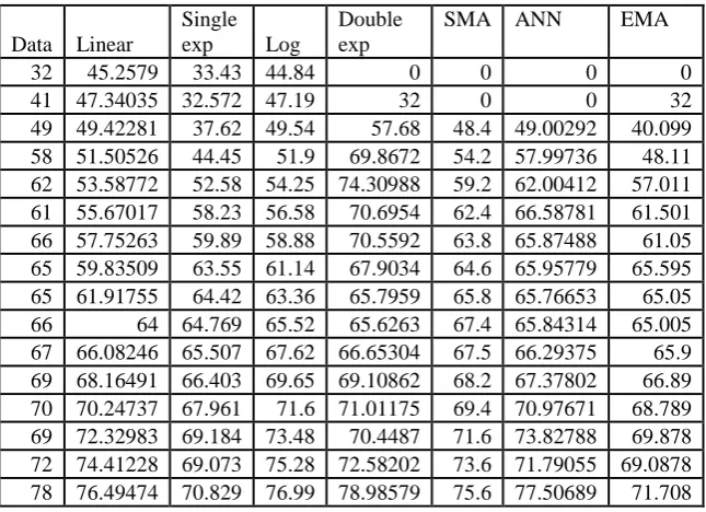
The following table shows the database of ratio of Girls per 100 boys enrolled in middle (VI-VIII) in India 1950 to 2005-06
Table 1: Result of Girls boys ratio in Middle (VI-VIII) Enrolled in India 1950 to 2005-06
Data Linear
Single exp Log
Double exp
SMA ANN EMA
Figure 2 graphically shows the comparison result of Girls enrollment per 100 boys in middle database.
Fig 2: Comparison result of different prediction method on girls boys ratio in middle database
The following table shows the result of residual analysis of different prediction technique on girls boys ratio enrolled in India at Middle(VI-VIII) 1950 to 2005-06.
Prediction Technique
Mean of Absolute Residual
Maximum Residual
Mean of Mean of Absolute
Residual
Median Absolute Residual
Standard Deviation
Linear 14 1.31 0.069 0.015 11.67
Logarithm 12.84 1.24 0.065 0.48 11.68 Single
exp 13.82 1.64 0.086 2.77 13.01 Double
exp 14.98 2.56 0.076 2.56 12.93
SMA 12.04 1.98 0.072 1.98 12.78
ANN 1.26 0.33 0.017 0.34 12.85
EMA 4.34 0.739 0.198 0.76 14.67
Table 2: Residual Analysis Girls boys ratio in Middle (VI-VIII) enrolled in India 1950 to 2005-06
The following table shows the database of ratio of Girls per 100 boys enrolled in Secondary (IX-X) in India 1950 to 2005-06
Figure3 graphically shows the comparison result of Girls enrollment per 100 boys in Secondary database.
Fig 3: Comparison result of different prediction method on girls boys ratio in Secondary database
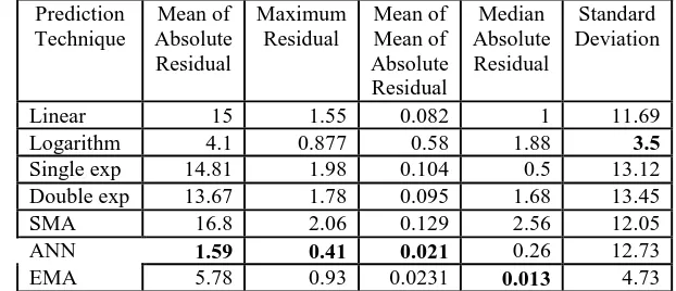
The following table shows the result of residual analysis of different prediction technique on girls boys ratio enrolled in India at Secondary (IX-X) 1950 to 2005-06.
Prediction Technique
Mean of Absolute Residual
Maximum Residual
Mean of Mean of Absolute Residual
Median Absolute Residual
Standard Deviation
Linear 15 1.55 0.082 1 11.69 Logarithm 4.1 0.877 0.58 1.88 3.5 Single exp 14.81 1.98 0.104 0.5 13.12 Double exp 13.67 1.78 0.095 1.68 13.45 SMA 16.8 2.06 0.129 2.56 12.05
ANN 1.59 0.41 0.021 0.26 12.73
EMA 5.78 0.93 0.0231 0.013 4.73
Table 4: Residual Analysis Girls boys ratio in Secondary (IX-X) enrolled in India 1950 to 2005-06
Table 5 shows the minimum error count of two different time series data in residual analysis. Data Set linear Single Exp Log Double Exp SMA ANN EMA Girls enrollment per
100 boys (Middle)
1 0 0 0 0 4 0
Girls enrollment per 100 boys
(Secondary)
0 0 1 0 0 3 1
Table 5: Minimum Error count of two different time series data in residual Analysis
IV.
CONCLUSION
Here in these paper different statistical methods, smoothing methods, Artificial Neural network is applied on two different time series datasets and on the basis of residual analysis we can conclude on the fact that ANN’s performance is best among other methods that has been used here.
V.
ACKNOWLEDGEMENT
Authors of this paper sincerely thank all the members of Information Technology Department of IIEST, Shibpur, Information Technology Department of KGEC, Kalyani and Purobi Das School of Information Technology Department, IIEST, Shibpur for their constant support and encouragement. Authors also sincerely thank the Institutions Authorities for their support.
REFERENCES
[1] G. A. Tagliarini, J. F. Christ, E. W. Page, “Optimization using Neural Networks, IEEE Transactions on Computers. vol. 40. no 12. December ’91,pp 1347-1358
[2] T. K. Bhattacharya and T. K. Basu, “Medium range forecasting of power system load using modified Kalman filter and Walsch transform”, Electric Power and Energy Systems”, vol. 15, no 2, pp109 -115, 1993.
[3] 26(1998),pp 275-281.
[4] J. V. Hansen and Ray D. Nelson, “Neural Networks and Traditional Time Series Methods: A Synergistic combination in state Economic Forecasts”, IEEE Transactions on Neural Networks vol. 8, no 4, July 1997