Aus dem Lehrstuhl für Neurophysiologie der Medizinischen Fakultät Mannheim
Centrum für Biomedizin und Medizintechnik Mannheim (Direktor: Prof. Dr. med. Rolf-Detlef Treede)
Optimizing the utility of Quantitative Sensory Testing for individual
diagnostics and development of a mechanism-based classification of
neuropathic pain.
Inauguraldissertation
zur Erlangung des Doctor scientiarum humanarum (Dr. sc. hum.) der Medizinischen Fakultät Mannheim
der Ruprecht-Karls-Universität zu
Heidelberg
vorgelegt von Jan Vollert aus Altena (Westf.)
Dekan: Prof. Dr. med. Sergij Goerdt Referent: Prof. Dr. med. Rolf-Detlef Treede
CONTENTS
Page
ABBREVIATIONS ... 1
1
INTRODUCTION ... 3
1.1 Pain and neuropathic pain ... 3
1.2 Peripheral sensory signal transduction ... 4
1.3 Nociception ... 4
1.4 Mechanisms of neuropathic pain ... 5
1.5 Sensory phenotyping ... 6
1.6 Aims and objectives ... 7
2
METHODS ... 10
2.1 Consortia and participating centers ... 10
2.2 Patient and participant selection ... 11
2.2.1 Patients ... 11
2.2.2 Healthy participants ... 12
2.2.3 Human surrogate models of neuropathic pain ... 12
2.3 QST protocol ... 13
2.4 z-transformation... 14
2.5 Analysis of heterogeneity ... 15
2.7.1 Simplified phenotyping ... 20
2.7.2 Discrimination analysis against healthy participants ... 20
2.7.3 Effectiveness for treatment with oxcarbazepine ... 21
2.8 Sample size recommendations... 22
2.9 Subgrouping human surrogate models ... 23
2.10 Patients in heuristic and mechanistic phenotypes ... 24
3
RESULTS ... 25
3.1 Patients and participants ... 25
3.1.1 Patients ... 25
3.1.2 Healthy participants ... 27
3.1.3 Human surrogate models ... 27
3.2 Analysis of heterogeneity ... 28
3.2.1 Healthy participants ... 30
3.2.2 Polyneuropathy ... 31
3.2.3 Peripheral nerve injury ... 31
3.3 Cluster analysis of patients ... 31
3.3.1 Sensory profiles of the three-cluster solution ... 33
3.3.2 Patient characteristics of the three clusters ... 35
3.3.3 Distribution of clusters across etiologies ... 39
3.4 Individual sorting algorithm ... 40
3.4.1 Sorting algorithm... 40
3.4.2 Discrimination analysis against healthy participants ... 41
3.4.3 Deterministic and probabilistic algorithm ... 43
3.4.4 Effectiveness for treatment with oxcarbazepine ... 44
3.5.1 Deterministic ... 47
3.5.2 Probabilistic ... 47
3.5.3 Simplified phenotyping ... 49
3.6 Sample size recommendations... 49
3.7 Subgrouping human surrogate models ... 51
3.7.1 Cluster analysis of human surrogate models ... 55
3.7.2 Pattern-based sorting algorithm ... 56
3.7.3 Deterministic and probabilistic sorting ... 58
3.8 Patients in heuristic and mechanistic phenotypes ... 60
4
DISCUSSION ... 64
4.1 Heterogeneity between centers ... 65
4.2 Sensory phenotypes in patients... 68
4.2.1 Sensory loss phenotype ... 69
4.2.2 Thermal hyperalgesia phenotype... 70
4.2.3 Mechanical hyperalgesia phenotype... 71
4.2.4 Sample size recommendations ... 71
4.3 Subgrouping human surrogate models ... 73
4.3.1 Nerve blocks as human surrogate model of denervation ... 73
4.3.2 Primary hyperalgesia as human surrogate model of peripheral sensitization ... 74
4.3.3 Secondary hyperalgesia as human surrogate model of central sensitization ... 74
4.3.4 Other human surrogate models ... 75
5
SUMMARY ... 81
6
REFERENCES ... 83
6.1 Publications that arose from the master thesis prefacing this work ... 96
6.2 Publications that arose from this work ... 96
7
LIST OF TABLES AND FIGURES ... 98
7.1 Tables ... 98 7.2 Figures ... 99
8
CURRICULUM VITAE ... 100
8.1 Publications ... 101 8.2 Oral presentations ... 103 8.3 Poster presentations ... 1049
ACKNOWLEDGMENTS ... 106
Abbreviations
ABBREVIATIONS
ARI Adjusted Rand Index AUC Area Under Curve
AVI Adjusted Variation of Information BIC Bayesian Information Criterion
BMBF German Federal Ministry for Education and Research CDT Cold Detection Threshold
CI Confidence Interval CPT Cold Pain Threshold
CRPS Complex Regional Pain Syndrome
DB Database
DET Deterministic algorithm
DFNS German Research Network on Neuropathic Pain DMA Dynamic Mechanical Allodynia
dPNP diabetic Polyneuropathy EM Expectation Maximization EMA European Medicines Agency H Healthy sensory profile
HFS electrical High-Frequency Stimulation HIV Human Immunodeficit Virus
HPT Heat Pain Threshold i.d. intradermal
IASP International Association for the Study of Pain IENFD Intra-Epidermal Nerve Fiber Density
Abbreviations
MDT Mechanical Detection Threshold MH Mechanical Hyperalgesia phenotype MPS Mechanical Pain Sensitivity
MPT Mechanical Pain Threshold
NB Nerve Block mechanistic phenotype NNT Number Needed to Treat
NPSI Neuropathic Pain Symptom Inventory
PH Primary Hyperalgesia mechanistic phenotype PHN Post-Herpetic Neuralgia
PHS Paradoxical Heat Sensation PiNS Pain in Neuropathy Study PNI Peripheral Nerve Injury PNP Polyneuropathy
PPT Pressure Pain Threshold QST Quantitative Sensory Testing RAD Radiculopathy
ROC Receiver Operating Characteristics
SH Secondary Hyperalgesia mechanistic phenotype SL Sensory Loss phenotype
TH Thermal Hyperalgesia phenotype TN Trigeminal Neuralgia
TRPV1 Transient Receptor Potential Vanilloid 1 TSL Thermal Sensory Limen
UVB Ultraviolet Radiation B
VDT Vibration Detection Threshold WDT Warm Detection Threshold WUR Wind-Up Ratio
Introduction
1 INTRODUCTION
1.1 Pain and neuropathic pain
Pain is defined as an “unpleasant sensory and emotional experience associated with actual or potential tissue damage, or described in terms of such damage” by the International Association for the Study of Pain (IASP) (Marskey et al., 1979). While acute pain serves as a warning and protective system activated by tissue damage or trauma, chronic and persistent pain may turn into a pathological state of its own (Loeser and Treede, 2008). If the pathophysiological basis is known, chronic pain can be subdivided into two major groups:
- Nociceptive pain is arising from activation of nociceptors (sensory neurons reporting actual or potential tissue damage). Chronic inflammation can lead to inflammatory pain, a chronic form of nociceptive pain. The nociceptive system itself is not directly affected, but may alter over time via sensitization (Loeser and Treede, 2008).
- Neuropathic pain results from an injury or disease to the nociceptive system (Treede et al., 2008; Finnerup et al., 2016) and can be caused peripherally (peripheral neuropathic pain) or in the central nervous system (central neuropathic pain).
Historically, peripheral neuropathic pain is classified based on the underlying disease or event initiating the nervous damage, such as diabetes, HIV, or chemotherapy-induced polyneuropathy (PNP), post-traumatic peripheral nerve injury (PNI), radiculopathy (RAD), trigeminal neuralgia (TN) or post-herpetic neuralgia (PHN) (Colloca et al., 2017). Treatment guidelines are often based on these etiologies, though it has become evident over the last decades that this approach is not sufficient, as first line treatment fails in over 50% of patients (Finnerup et al., 2015; Bouhassira and Attal, 2016). While written ten years ago, the following devastating statement remains largely valid: “The management of patients with chronic NP
[neuropathic pain, A/N] is complex and response to existing treatments is often inadequate. Even with well-established NP medications, effectiveness is unpredictable, dosing can be complicated, analgesic onset is delayed, and side
Introduction
The fact that common symptoms and signs of neuropathic pain appear across etiologies, while varying in pattern within etiologies, has led to the idea that distinct pathogenic mechanisms of neuropathic pain appear across etiologies (Fields et al., 1998; Woolf and Mannion, 1999; Campbell and Meyer, 2006; Baron et al., 2012; von Hehn et al., 2012). Treatment of neuropathic pain therefore should be aiming at mechanisms rather than at etiology.
1.2 Peripheral sensory signal transduction
The somatosensory (nervous) system comprises the afferent peripheral sensory receptor neurons, and their subsequent second-order neurons in the central nervous system (Kandel et al., 2013). All afferent sensory receptor neurons are pseudo-unipolar neurons based in the dorsal root (or trigeminal) ganglia with a single axon that divides at a T-junction into a peripheral axon, innervating skin or deep tissue, and a central axon, transmitting signals onto secondary neurons in the spinal cord or medulla oblongata (Squire et al., 2008). Sensory neurons differ, however, in degree of myelination, and (conclusively) signal conduction velocity (Kandel et al., 2013). Three major fiber types can be distinguished in primary afferent neurons:
- Aβ-fibers – thickly myelinated (nerve fiber diameter 6 – 12 μm), high conduction velocity (36 – 72 m/s) (Kandel et al., 2013) – innervate cutaneous mechanoreceptors (e.g. vibration, pressure) (Squire et al., 2008),
- Aδ-fibers – thinly myelinated (nerve fiber diameter 1 – 6 μm), medium conduction velocity (3 – 36 m/s) (Kandel et al., 2013) – detect cold and noxious stimuli (Squire et al., 2008) and
- C-fibers – unmyelinated (nerve fiber diameter 0.2 – 1.5 μm), slow conduction velocity (0.4 – 2 m/s) (Kandel et al., 2013) – transmit warm and noxious stimuli (Squire et al., 2008).
1.3 Nociception
Noxious stimuli are transduced (e.g. via TRPV1) and subsequently transformed into action potential trains (e.g. via NaV 1.7, 1.8, etc.). These trains are conducted via small, thinly or unmyelinated Aδ- or C-fibers. The divergent conduction velocity of these fibers results in the concept of first and second pain: the former, conducted by
Introduction
faster Aδ-fibers, is discriminative and rapidly induces efferent response, the latter, conducted by slower C-fibers, is less localized and of longer duration (Squire et al., 2008).
Nociceptors with Aδ-fibers are sensitive to either mechanical stimuli and induce pain of sharp or pricking quality, or are sensitive to mechanical and heat stimuli and induce pain of burning quality (Kandel et al., 2013). Nociceptors innervated by C-fibers are polymodal or sensitive to mechanical and cold stimuli and induce pain of burning or freezing quality (Kandel et al., 2013). It should be noted that the majority of nociceptors are polymodal and respond to various stimuli, such as heat, cold, sharp or blunt pressure, or chemicals, but the sensitivity spectrum varies broadly between nociceptors (Kandel et al., 2013).
1.4 Mechanisms of neuropathic pain
According to a recent review (Colloca et al., 2017), along the nociceptive pathways, at three levels the generation of neuropathic pain can take place:
1. First-order nociceptor ion channels (peripheral sensitization).
Altered function of transduction channels (e.g. TRPV1 (Haanpaa and Treede, 2012)), as well as in- or decreased activity or expression of sodium, potassium and/or calcium channels in affected afferent nerves can induce spontaneous pain or hyperexcitability of the affected nerves, which has been shown for example in case of congenital overexpression of sodium channels, which can induce painful diseases like erythromelalgia (McDonnell et al., 2016). Similarly, increased sodium or decreased potassium channel function can induce hyperexcitable nociceptors (often called IN = irritable nociceptors) (Fields et al., 1998; Tesfaye et al., 2013). These can also cause spontaneous pain via ectopic activity. Increased pain sensitivity due to peripheral sensitization is limited to the site of injury, trauma or disease and called primary hyperalgesia (Treede et al., 1992; Hucho and Levine, 2007).
2. Second-order neurons (central sensitization).
Enhanced excitability of second order nociceptive neurons can increase their response to nociceptor input and widen their receptive field so that input from
Introduction
accounts for secondary hyperalgesia (pain increased in spatial extend beyond the initial area of the injury or disease) and allodynia (painful sensation to non-painful stimuli) (Baron et al., 2013).
3. Inhibitory modulation.
Descending modulatory pathways and inhibitory interneurons can be impaired in patients with neuropathic pain, shifting the balance between pain inhibition and excitation further towards excitation (Colloca et al., 2017). It has been shown that the extent of conditioned pain modulation, where the perceived pain intensity of a steady painful test stimulus is reduced by applying a second tonic painful stimulus, is reduced in many patients with chronic pain (Lewis et al., 2012).
These mechanisms are, as stated above, present across etiologies of neuropathic pain (though varying in frequency), they may co-exist and enhance or facilitate each other, and, most importantly, are assumed to respond to distinct forms of treatment (Finnerup et al., 2015). Therefore, a mechanistic classification of neuropathic pain has been under debate for over 25 years now (Fields et al., 1998; Woolf et al., 1998; Baumgartner et al., 2002; Baron et al., 2012; von Hehn et al., 2012; Edwards et al., 2016).
1.5 Sensory phenotyping
To establish a mechanism-based classification, it is crucial to be able to detect and describe the mechanisms involved in the generation of pain in the individual patient. A first step can be patient-recorded questionnaires, capturing subjective reports of dimensions of neuropathic pain like the Neuropathic Pain Symptom Inventory (NPSI) (Bouhassira et al., 2004). As a second step, bedside testing of sensory signs like loss of thermal or mechanical detection or painful reaction to stimuli that are normally not perceived as painful may indicate involvement of mechanisms. However, both methods are subjective and hardly comparable between patients.
A comprehensive way to capture a patient’s sensory function is Quantitative Sensory Testing (QST) (Krumova et al., 2012a). When performed in accordance with the DFNS (German Research Network on Neuropathic Pain) protocol (Rolke et al., 2006b), QST assess thermal and mechanical detection and pain thresholds, capturing various aspects of neuropathic pain:
Introduction
1. Denervation/deafferentation – increased detection thresholds indicate loss of activity and/or presence of Aβ- (mechanical detection), Aδ- (cold detection) or C-fiber sensory neurons.
2. Peripheral sensitization – heat hyperalgesia or increased deep pain sensitivity to blunt pressure in combination with unimpaired thermal detection may indicate irritable nociceptors.
3. Central sensitization – dynamic mechanical allodynia, increased pinprick pain sensitivity and cold hyperalgesia indicate central sensitization.
4. Modulatory descending pathways – an increased wind-up ratio (rating of a single painful stimulus compared to a series of ten such stimuli) indicates impaired descending noxious inhibition controls.
While QST has shown its capacity to identify and separate groups of patients with neuropathic pain (Maier et al., 2010; Smith et al., 2017), its usefulness for individual treatment is under discussion (Hansson et al., 2007; Backonja et al., 2013). Detection and pain thresholds vary broadly within healthy populations, and are influenced by age, gender, tested body region, and more problematic, by many factors that are impossible to control for, like genetics, epigenetics and individual development. Still, this is a frequent phenomenon in medicine and even more problematic in other tests assessing the nervous system (e.g. counting intraepidermal nerve fibers after skin biopsy (Isak et al., 2017)).
1.6 Aims and objectives
The European consortia IMI (Innovative Medicines Initiative) Europain, Neuropain and the DFNS have gathered QST data of 945 patients with peripheral neuropathic pain and 657 healthy participants with transient sensory changes due to surrogate models for neuropathic pain. In addition, reference data of healthy participants was collected in the DFNS (Rolke et al., 2006a; Blankenburg et al., 2010; Magerl et al., 2010; Pfau et al., 2014; Vollert et al., 2016a), and 188 healthy participants from additional German and European centers were included subsequently (Vollert et al., 2016a). All data have been collected in a central database in Bochum, Germany (Maier et al., 2010; Vollert et al., 2016a; Baron et al., 2017; Vollert et al., 2017b).
Introduction
with high data quality was the central task of my master thesis (Vollert et al., 2015; Vollert et al., 2016b), scope of the present thesis was to adapt, develop and perform all mathematical analysis necessary to develop an individual algorithm to assign patients to sensory phenotypes that are linked to mechanisms of pain generation. En detail, aim of this work was to use this data to:
1. Perform a systematic analysis of heterogeneity of QST assessment of patients and healthy participants between the participating European centers, to show that comparability between centers is guaranteed, a central prerequisite for analyzing the data as a homogenous dataset.
2. Use unsupervised clustering methods to identify subgroups of sensory profiles appearing across etiologies of peripheral neuropathic pain and may indicate underlying mechanisms of pathophysiology.
3. Develop an algorithm that enables assignment of individual patients to one or more of the subgroups identified in (2) based on the patient’s QST profile. 4. Apply the algorithm from (3) to 83 patients with peripheral neuropathic pain,
whose pain relief after treatment with oxcarbazepine is known from a former study (Demant et al., 2014). Oxcarbazepine blocks sodium channels that are mainly located on small nerve fibers, and is therefore thought to be ineffective in patients with pain linked to deafferentation. In their study, Demant et al. found that patients with intact thermal detection show a significantly increased pain relief after treatment with oxcarbazepine compared to patients with loss of thermal detection. A pain relief that is significantly higher in a sensory subgroup from (2) with intact thermal detection compared to those with loss of thermal detection would indicate mechanistic variance in pain generation between subgroups.
5. Apply the algorithm from (3) to 335 patients with painful peripheral nerve injury, 151 patients with painful diabetic neuropathy, and 97 patients with post-herpetic neuralgia. Based on the frequency of each phenotype in each etiology, sample sizes of study populations that need to be screened to reach a sub-population large enough to conduct a phenotype-stratified study were to be calculated.
6. To create a database of human surrogate models studied with full QST profiles and to perform a similar cluster analysis and a similar individual algorithm as in (3) in 657 healthy participants with transient sensory changes
Introduction
due to surrogate models for denervation, peripheral sensitization and central sensitization. These represent well-studied mechanisms.
7. To further validate the phenotypes identified in (2) by submitting them to the mechanism-based individual algorithm developed in (6). An emergence of similar phenotypes in surrogate models that are similar in mechanism would further strengthen the concept of sensory phenotypes representing mechanisms of neuropathic pain.
Methods
2 METHODS
2.1 Consortia and participating centers
The DFNS (http://www.neuropathischer-schmerz.de) was formed in 2002 and financed by a BMBF (federal ministry for education and research) grant to investigate mechanisms and treatments of neuropathic pain. Forming universities were the Ruhr University, Bochum, University of Schleswig Holstein, Kiel, Technical University, Munich, Ruprecht-Karls-University, Heidelberg, Johannes-Gutenberg-University, Mainz, University of Erlangen, University of Tübingen, University of Würzburg, University of Ulm. The study protocol was approved by the ethics committee of the University Hospital Kiel and subsequently by the ethics committees of all participating centers. Subsequently, the University Hospital of the Goethe-University, Frankfurt am Main, joined the DFNS and participated in collecting data from human surrogate models of neuropathic pain.
The EUROPAIN project (http://www.imieuropain.org) was founded in 2009 and financed by the European union’s seventh framework programme. Data for this study were collected by the following centers: Aarhus University, Denmark, Ruhr-University, Bochum, Germany, University of Schleswig Holstein, Kiel, Germany, Technical University, Munich, Germany, Medical Faculty Mannheim, Ruprecht-Karls-University, Heidelberg, Germany. The ethics committee of each center approved the study protocol individually.
The NEUROPAIN project is an investigator-initiated project sponsored by Pfizer. Data for this study were collected by the following centers: Aarhus University, Denmark, Ruhr-University Bochum, Germany, University of Schleswig Holstein, Kiel, Germany, Technical University, Munich, Germany, Medical Faculty Mannheim, Ruprecht-Karls-University, Heidelberg, Germany, Université Versailles-Saint-Quentin, Versailles, France, Sapienza University, Rome, Italy, Helsinki University Central Hospital, Finland, Karolinska Institutet, Stockholm, Sweden, Benedictus Hospital Tutzing, Germany, Imperial College, London, United Kingdom, Neuroscience Technologies, Ltd., Barcelona, Spain. The ethics committee for each center approved the study protocol individually.
Methods
The Pain in Neuropathy Study (PiNS) was supported by the Wellcome Trust, and the European Union's Horizon 2020 research and innovation program. Data for this study were collected at the Oxford University, Oxford, United Kingdom, Imperial College, London, United Kingdom, and Sheffield Teaching Hospitals, Sheffield, United Kingdom. The ethics committee for each center approved the study protocol individually.
All participating centers underwent strict quality control (Geber et al., 2009; Magerl et al., 2010; Vollert et al., 2015) to ensure comparability of QST assessments between centers.
2.2 Patient and participant selection
2.2.1 Patients
[The following section has been taken in parts and modified from (Vollert et al., 2016b) and (Baron et al., 2017).]
Inclusion criteria for patients were carefully checked by a physician experienced in pain medicine at the local center. For each diagnosis, inclusion criteria were as follows:
- Polyneuropathy: pathological electroneurography or pathologically decreased vibration detection thresholds at two of four sites (< 5/8) at the lower limb, which could not be explained by another disease, or pain with polyneuropathy-type location and evidence of small fiber neuropathy based on skin punch biopsy, laser-evoked potentials or bedside thermal testing, which could not be explained by another disease.
- Peripheral nerve injury: history of traumatic nerve injury of the distal upper or lower limb and sensory-motor abnormalities confined to the innervation territory of the injured nervous structure or idiopathic sensory trigeminal neuropathy or iatrogenic mandibular neuropathy (i.e., inferior alveolar or lingual nerve neuropathy after various kinds of intraoral procedures) or trigeminal neuropathy secondary to compression, trigeminal neuropathy
Methods
- Post-herpetic neuralgia: unilateral zoster rash in the facial or thoracic area with post-zoster scarring, hypo- or hyperpigmentation in the affected dermatome or sensory deficit around the previous zoster rash determined by bedside-testing. - radicular lesion: pain in the L5 and/or S1 dermatome and positive straight leg raising test or sensory deficit within the matching dermatome or diminished Achilles tendon reflex for S1 lesions and MRI of the lumbar spine confirming nerve root impairment by a herniated intervertebral disk or electromyography showing denervation in the L5 or S1 territory.
Exclusion criteria were age under 18 years, missing informed consent, insufficient language skills or other communication problems, pain treatment by topical local anesthetics for ≥ 7 days in the last 4 months or by topical capsaicin in the last 6 months, comorbidities treated by anticonvulsants or antidepressants, other pain locations with pain intensities ≥ 6 on ≥ 15 days/ month, other severe systemic or focal diseases of the central nervous system (e.g., stroke, spinal cord lesion), spinal canal stenosis, peripheral vascular disease (Fontaine stage II or higher), pending litigation and major cognitive or psychiatric disorders. In the cases of unilateral pain syndromes, contralateral neuropathies or painful conditions of the contralateral limb had to be excluded. Datasets were excluded in the case of incomplete records (e.g., no precise diagnosis available, more than 2 missing variables of the QST in the affected area, no information about age, gender or other demographic data).
2.2.2 Healthy participants
Healthy participants were included based on the recommendations by Gierthmühlen et al. (Gierthmuhlen et al., 2015) and collected by ten centers from the DFNS, IMI Europain and Neuropain for quality assurance purposes (Vollert et al., 2015) during the certification process of these centers (Geber et al., 2009).
2.2.3 Human surrogate models of neuropathic pain
The following human surrogate models for neuropathic pain were conducted within the DFNS and included in the analysis (Klein et al., 2005; Vollert et al., 2017b):
- A-fiber-block (unpublished data collected in Kiel and Mannheim, methods as in (Ziegler et al., 1999)). Selectively blocking A-fibers leads to strongly decreased
Methods
sensory function (except warm detection, which is C-fiber mediated) and is a model for selective deafferentation/denervation of myelinated nerves (e.g. demyelinating polyneuropathy).
- Topical lidocaine cream application. Topical lidocaine induces loss of sensory function and therefore is a model of denervation/deafferentation (Krumova et al., 2012b).
- Topical capsaicin application, using cream, watery solution, or patch. The application of topical capsaicin induces peripheral sensitization, and can lead over time to a secondary hyperalgesia beyond the immediately affected area, a model for peripheral sensitization leading to central sensitization (Baron et al., 2013; Lotsch et al., 2015)
- UV-B light irradiation (unpublished data collected in Mannheim and published data, methods as in (Gustorff et al., 2013)). The sunburn model induces primary and secondary hyperalgesia similar to topical capsaicin (Gustorff et al., 2013)
- Intradermal capsaicin injection (unpublished data collected in Kiel, Mannheim and TU Munich, methods as in (Magerl and Treede, 2004). The injection leads to secondary hyperalgesia, without inducing primary hyperalgesia first (Magerl and Treede, 2004).
- Cutaneous electrical high-frequency stimulation (HFS). Cutaneous HFS leads to mechanical hyperalgesia and allodynia, and therefore is a model of central sensitization (Lang et al., 2007).
- Muscular electrical high-frequency stimulation. HFS in the muscle is thought to lead to peripheral sensitization (Schilder et al., 2016).
- Topical menthol application. As topical menthol application leads to primary and secondary cold and mechanical hyperalgesia, it is a model for central sensitization (Wasner et al., 2004; Binder et al., 2011).
- Topical application of capsaicin solution in combination with lidocaine patch. This model induces primary hyperalgesia (peripheral sensitization) in combination with loss of function, e.g. numbness (Enax-Krumova et al., 2017).
Methods
alternating cold and warm stimuli and the number of paradoxical heat sensations (PHS) during this procedure, cold and heat pain thresholds (CPT and HPT, respectively), tactile (mechanical) detection threshold (MDT), mechanical pain threshold and sensitivity to pinprick stimuli (MPT, MPS), dynamical mechanical allodynia to touch with a brush, cotton wool or Q-tip (DMA), the wind-up ratio (WUR) of the perceived pain of a single pinprick stimuli compared to a series of ten stimuli, vibration detection threshold (VDT) and deep pain sensitivity to blunt pain (pressure pain threshold, PPT) (Rolke et al., 2006a).
Thermal sensory and pain thresholds were performed using either a TSA 2001-II (MEDOC, Israel) or a MSA (SOMEDIC, Sweden) that in- or decreased temperature by 1°C per second (Rolke et al., 2006b). For the TSL, six warm and cool stimuli were applied. The participant was asked whether he or she felt a cold or a warm stimulus, and the number of PHS (warm sensations during cold stimuli) was recorded. MDT was defined as the geometric mean of 5 series of stimuli ascending and descending between 0.25 and 512mN by a standardized set of von Frey hairs, mechanical pain threshold as the geometric mean of 5 series of stimuli ascending and descending by applying pinprick stimuli between 8 and 512mN (Rolke et al., 2006b). MPS and DMA were assessed by applying a total of 50 stimuli (35 pinprick and 15 light tactile in a balanced protocol) and asking patients to give a pain rating on a 0 (no pain) to 100 (worst pain imaginable) NRS scale. MPS was calculated as the geometric mean of the pain ratings of the pinprick stimuli, DMA as the geometric mean of the pain rating of the tactile stimuli. For the WUR the perceived intensity of a single pinprick stimulus was compared with that of a series of 10 repetitive pinprick stimuli of the same physical intensity on a 0-100 NRS scale, as an average of five series (Rolke et al., 2006b). VDT was assessed with a Rydel–Seiffer graded tuning fork (64 Hz, 8/8 scale, mean of three testing series) and PPT was determined over muscle with a pressure gauge device (FDN200, Wagner Instruments, USA), exerting forces up to 2000 kPa, as a mean of three series of ascending stimulus intensities, each slowly increasing (50 kPa/s) (Rolke et al., 2006b).
2.4 z-transformation
The initial assessment of 180 healthy participants for the DFNS reference database revealed that all parameters except PHS and DMA could be transformed (partly in
Methods
log-space) to a standard normal distribution (Rolke et al., 2006a; Magerl et al., 2010; Pfau et al., 2014). This process, called z-transformation, normalizes all values to a mean = 0 and a standard deviation = 1. Subsequently, all QST results of patients and healthy participants were transformed in accordance to this normalization. The z-transformation normalizes for age decade, gender and tested body region, thus making pain and detection thresholds comparable between patients with different age and gender, with nerves affected e.g. at the face or the feet. Abnormal values are defined as values beyond the 95% confidence interval. While individual z-scores are considered as abnormal if beyond ± 1.96 (Rolke et al., 2006a), for groups of patients, z-scores of ± 1.0 have been shown to be of clinical significance, as they include a relevant number of patients with abnormal values (Maier et al., 2010). DMA and PHS, which do not normally occur in healthy participants, cannot be z-transformed. They are usually presented as percentages of presence, but for use in statistical analysis, they can be transformed to pseudo-z-values: DMA can be coded into a 0/2/3-variable representing no DMA (coded as 0), DMA with average pain ratings below 1 on a 0-100 NRS scale (coded as +2) and DMA with average pain ratings between 1 and 100 (coded as +3). PHS can be transformed to a binary 0/2-variable showing absence (coded as 0) or presence (coded as +2) of pathological values (Baron et al., 2017).
As many surrogate models were applied at the volar lower arm or upper thigh, which are not standardized areas, data of the subjects tested in the same area before treatment, or, if this data was unavailable, of the contralateral untreated side was compared used to calculate effect sizes (Cohen’s d (Cohen, 2013)). This measure normalizes changes in the mean value before and after treatment to standard deviation, i.e. an effect size = 1 equals a change in the mean value after treatment that is equal to the standard deviation of the sample. There are no general interpretations of “good” effect sizes, but it is often considered that effect sizes below 0.3 can be considered small, and above 0.7 can be considered as large treatment effects (Cohen, 1992).
Methods
To assess the variability of QST results across the different centers, random effects models for the eleven normally distributed QST parameters were adopted, with the QST z-value of a certain parameter as the dependent variable and center as the random effect. For the analysis of cold detection thresholds in patients suffering from polyneuropathy, let 𝑌𝑖𝑗 be the CDT z-value of 𝑗th patient (1 ≤ 𝑗 ≤ 𝑁) in the 𝑖th center (1 ≤ 𝑖 ≤ 𝑀), the model is specified as:
𝐹(1): 𝑌𝑖𝑗 = 𝜇 + 𝛼𝑖+ 𝜀𝑖𝑗 𝐹(2𝑎): 𝜀𝑖𝑗 ~ 𝑁(0, 𝜎2)
𝐹(2𝑏): 𝛼𝑖 ~ 𝑁(0, 𝜎𝜇2)
where 𝜇 is the overall mean CDT z-value across all centers, 𝑎𝑖 is the unobserved center-specific random effect and ɛ𝑖𝑗 is the individual unexplained effect. The model is fitted so that 𝜀𝑖𝑗 and 𝑎𝑖are normally distributed with a mean value = 0 (F(2a) and F(2b)). The estimated center-specific mean z-values (𝜇 + 𝑎𝑖 for 1 ≤ 𝑖 ≤ 𝑀) and the corresponding 95% confidence intervals from Model (1) are graphically displayed in forest plots separately for PNP, PNI and healthy participants, with the Y-axis showing a running number for the centers for all 11 QST parameters and the X-axis presenting the center-specific mean z-value. The I² statistic (Higgins and Thompson, 2002) was employed to quantify the heterogeneity of mean z-values across the centers. This statistic ranges from 0 to 100% and it measures the percentage of variation across studies that is due to true heterogeneity rather than chance. The confidence interval estimates of I² were computed based on the test-based method of Higgins and Thompson (Higgins and Thompson, 2002).
2.6 Cluster analysis protocol
[The following section has been taken in parts and modified from (Baron et al., 2017).]
A cluster analysis was performed to unravel distinguishable subgroups of QST-profiles. The procedure of this analysis was identical for patients suffering from peripheral neuropathic pain (Baron et al., 2017) and healthy participants under conditions that induce human surrogate models of neuropathic pain, in order to
Methods
guarantee comparability between the results. We made no a-priori-assumptions about the expected number of clusters and applied a k-means-approach for a number of k clusters ranging from 2 to 10 (MacQueen, 1967). A two-step protocol was used to determine the optimum number of clusters:
- Negative silhouettes as exclusion criterion. A silhouette width is a value that can be calculated for each subject in each cluster and ranges between -1 and +1 (Rousseeuw, 1987). Positive values near +1 indicate a subject that can unambiguously be allocated to a certain cluster, values near zero indicate subjects that are on the edge between clusters, and negative values indicate that these subjects are allocated to a cluster that is not their nearest cluster. This is possible because if they would be allocated to their nearest cluster, the cluster mean would shift so that other subjects are then in a cluster that is not their nearest. A mean silhouette width well above zero for a cluster indicates that said cluster is clearly separated from the others, while a mean silhouette width below zero indicates a cluster that is rather a statistical artifact than a real subgroup. Therefore, a high count of negative silhouettes or a cluster with a mean silhouette width below zero indicate a cluster solution that is highly fragmented. Thus, to control for statistical artefacts, we excluded all solutions with at least one cluster with a negative mean silhouette width, and all solutions with over 10% negative silhouette widths.
- Comparability between clustering methods. The remaining solutions were compared to two additional cluster methods with significantly different mathematical background, validating that the final solution is not dependent on the clustering method. We decided on a robust hierarchical clustering method (maximum linkage) and an Expectation Maximization (EM) algorithm (Dempster et al., 1977). Both solutions were compared to the initial k-means clustering, using the adjusted rand index (ARI) and the adjusted variation of information (AVI). While the ARI measures similarity on a scale from 0 – 1 (high values are preferable), the AVI measures dissimilarity on the same scale (low values are preferable) (Rand, 1971). Final criterion for the decision between otherwise equal cluster solutions was the Bayesian Information Criterion (BIC) which captures the gain of information by increased number of
Methods
difference between the BICs of both solutions (Delta-BIC) is larger than ten (Schwarz, 1978).
2.6.1 Validation sets
To investigate the stability of the findings, for both cluster analyses (patients and surrogate models) a validation set was formed, in which additional k-means cluster analyses were performed, with a fixed number of clusters (as defined above).
For patients suffering from peripheral neuropathic pain, this validation set was formed from patients with PNP, PNI and PHN who were collected either within the DFNS after closure of the initial database (Maier et al., 2010) or within the Europain consortium for treatment studies with oxcarbazepine and lidocaine (Demant et al., 2014; Demant et al., 2015).
For human surrogate models of neuropathic pain, no similar cohort was available. Therefore, 50% of all data (chosen by random number assignment) were excluded from the initial analysis to form the validation set.
2.7 Individual sorting algorithm
[The following section has been taken in parts and modified from (Vollert et al., 2017a).]
As QST z-values are (per definition) normally distributed, our approach was based on normally distributed probabilities. For each QST z-value of each parameter i and patient n, a probability can be calculated for a phenotype to be present based on the density function of said phenotype:
𝐹(3): 𝑝𝑖𝑛,𝑚 = 1 √2𝜋𝜎𝑖𝑚2 exp ( − ( (𝑥𝑖𝑛−𝜇𝑖𝑚)² √2𝜎𝑖𝑚2 ))
With i = one of 13 QST parameters, n = the nth patient in a set of patients, m = one of the phenotypes determined in the cluster analysis of patients described above and conclusively, 𝜎𝑖𝑚 being the standard deviation of the ith QST parameter for the mth phenotype in the defining dataset (Baron et al., 2017), 𝜇𝑖
Methods
the same QST parameter and phenotype in the defining dataset (Baron et al., 2017), and finally 𝑥𝑖𝑛 being the z-value found in the nth patient for the ith QST parameter. While this function will always reach its maximum at 𝑥𝑖𝑛 = 𝜇𝑖
𝑚, in relation to
broadness of the standard deviation, density functions can become broader or narrower. This affects the maximum value the density function can reach. To control for these more or less broad functions, we normalized the formula so that a value that is equal to the mean of the phenotype equals 100%, leading to
𝐹(4): 𝑝𝑖𝑛,𝑚∗ = 1 √2𝜋𝜎𝑖𝑚2 exp ( − ( (𝑥𝑖𝑛−𝜇𝑖𝑚)² √2𝜎𝑖𝑚2 )) ⁄ 1 √2𝜋𝜎𝑖𝑚2 exp ( − ( (𝜇𝑖𝑚−𝜇𝑖𝑚)² √2𝜎𝑖𝑚2 ))
which can be simplified to
𝐹(5): 𝑝𝑖𝑛,𝑚∗ = exp ( − ( (𝑥𝑖𝑛−𝜇𝑖𝑚)² √2𝜎𝑖𝑚2 ))
The resulting probability value is ranging from 0% to 100% and can be calculated for all i = 13 QST parameters and m phenotypes. By averaging the probability over the 13 QST parameters, we quantify the similarity of the individual patient’s QST profile to the mean profile of each of the phenotypes.
As a simple way of categorizing patients into phenotypes, we suggest sorting each patient to the phenotype with the highest probability value:
1. Calculate F(5) for each of the 13 QST parameters. Use μ and σ for phenotype 1.
2. Average the 13 probabilities. The resulting value is the probability for this patient to show this phenotype.
3. Repeat steps 1 and 2, using μ and σ for the next phenotype. Repeat for all phenotypes.
Methods
2.7.1 Simplified phenotyping
As the DFNS protocol is comprehensive, it might be too complex to be applied in all clinical settings and in large clinical trials. If the cluster analysis showed that few parameters explain large parts of the variance between the discovered phenotypes, the accuracy of a phenotyping based on these in comparison to a phenotyping using the full protocol is analyzed.
2.7.2 Discrimination analysis against healthy participants
To show if and how the algorithm can discriminate patients with neuropathic pain from healthy participants, we introduced a fourth probability - not for a phenotype, but for being healthy. For this purpose, we applied the definition of QST z-values, to which a group of healthy participants ideally has a z-value mean = 0 (μ) with a standard deviation = 1 (σ) for each QST parameter. The original cluster patient cohort (Baron et al., 2017) (n = 902) and n = 188 healthy participants from the European cohort (Vollert et al., 2016a) underwent a modified version of the algorithm:
1. Calculate F(5) for each of the 13 QST parameters. Use μ and σ for healthy. 2. Average the 13 probabilities. The resulting value is the probability for this
patient to show a healthy profile.
3. Repeat steps 1 and 2, using μ and σ for all phenotypes.
As this version of the algorithm does not sort each subject simply to the phenotype with the highest probability, this leaves every subject with a series of probabilities, one for each of the phenotypes of neuropathic pain, and one for being healthy.
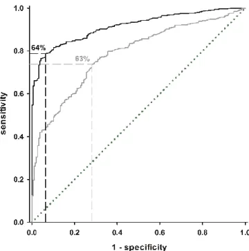
The probability of being healthy was used for a Receiver Operating Characteristics (ROC) plot (Zweig and Campbell, 1993). This graphical tool for assessing discriminatory power plots the false-positive rate (1 - specificity) on the x-axis versus the sensitivity of detecting patients on the y-axis for all possible probability values of being healthy. Each step in the ROC plot represents the specificity and sensitivity of one certain percentage. To assess the overall quality of separating healthy participants and patients via the probability for being healthy, the area under curve (AUC) and its 95% confidence interval were calculated (DeLong et al., 1988). To define a minimum probability, at which a subject should be considered being healthy,
Methods
the probability with the highest Youden-Index (sensitivity minus false-positive rate (Youden, 1950)) was chosen.
2.7.3 Effectiveness for treatment with oxcarbazepine
It has been shown in a recent study that the effectiveness of oxcarbazepine as treatment for neuropathic pain is dependent on the sensory phenotype of the patients (Demant et al., 2014). Oxcarbazepine is a blocker of voltage-gated sodium channels (McLean et al., 1994) and therefore has the potential to reduce neuropathic pain caused by overexpression or increased sensitivity of sodium channels (Ichikawa et al., 2001). This effect is, however, only possible in patients where this specific mechanism is present, and oxcarbazepine will therefore not help patients whose pain is generated more centrally (Katz et al., 2008). In their paper, Demant et al. phenotyped the patients as “irritable nociceptor” (IN, intact thermal detection, thermal or mechanical hyperalgesia) and “non-irritable nociceptor” (the remainder) (Demant et al., 2014). It was found that pain reduction was only significant in patients with “irritable nociceptor” phenotype. The number-needed-to-treat (number of patients that has to be treated with oxcarbazepine to find at least one patient with a pain reduction of at least 50% (Tramer and Walder, 2005)) was found to be 3.9 (95% CI: 2.3 – 11.5) for irritable nociceptor and 13.0 (95% CI: 5.2 - ∞) for non-irritable nociceptor. Using the original data provided by the principal investigators, the cohort underwent the individual algorithm to determine each patient’s cluster-based sensory phenotype. Based on mechanistic assumptions for the phenotypes identified in the previous steps, a hypothesis was formed which phenotype would respond to oxcarbazepine treatment. The treatment outcome was compared between cluster-based phenotypes and irritable/non-irritable nociceptor phenotyping, to analyze whether cluster-based phenotyping is similarly effective as (and non-inferior to) irritable/non-irritable nociceptor phenotyping as predictor for effectiveness of oxcarbazepine.
Three metrics were applied to show cluster-based phenotype-specificity of oxcarbazepine-related pain relief and to compare treatment prediction between phenotyping methods (cluster-based vs. irritable/non-irritable nociceptor):
Methods
model in the published study (Demant et al., 2014). This model was tested for both deterministic and probabilistic phenotyping.
- Mean pain reduction in the verum phase. The pain reduction between baseline and week six in the verum phase for IN patients and patients with a cluster-based phenotype that indicates effectiveness of oxcarbazepine was compared (two-tailed t-test). Cluster-based phenotyping was considered effective in case of a non-significant test or a significant test in combination with higher mean pain relief in the cluster-based phenotype compared to IN (non-inferiority). - Number-needed-to-treat. The NNT was calculated for the cluster-based
phenotype along with its 95% confidence interval (Tramer and Walder, 2005). Cluster-based phenotyping was considered effective in case of a lower NNT in the cluster-based phenotype compared to IN or a higher NNT with CIs overlapping between the NNTs for IN and cluster-based phenotyping (non-inferiority).
2.8 Sample size recommendations
[The following section has been taken in parts and modified from (Vollert et al., 2017a).]
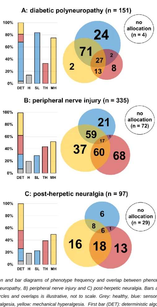
If a new drug would be tested for efficacy in a phenotype-stratified subgroup with neuropathic pain of any single etiology, this would only be feasible if said phenotype appears in a relevant frequency within this etiology. To show how frequent these phenotypes are across three common etiologies of neuropathic pain, we applied the algorithm to patients suffering from neuropathic pain due to diabetic polyneuropathy, peripheral nerve injury or post-herpetic neuralgia from the databases of our previous studies (Maier et al., 2010; Demant et al., 2014; Demant et al., 2015; Themistocleous et al., 2016; Baron et al., 2017).
Based on the frequencies found in the clinical entities, we calculated the size of a group of patients that need to be screened with either full or simplified phenotyping to find a sub-population large enough to perform a trial that still reaches a power of 80% for an effect size of 0.3, 0.5 and 0.7 at an alpha-level of 0.05, for a crossover and parallel design. The sample sizes presented in this thesis are examples and can be tailored to the needs of any planned RCT. We recommend the usage of the free software G*Power (Faul et al., 2007), but many other statistical packages provide
Methods
similar tools. The following information is required before starting: alpha-level (usually 0.05), power (usually 0.8, 0.9 or 0.95), test family (usually t-test for independent (parallel design) or dependent (crossover design) means, or chi-squared for dichotomous outcome), and the estimated effect size in the phenotype of interest. Effect sizes are related to mean treatment effect and standard deviation between treatment response, e.g., a mean effect of 2 on a 0-10 NRS scale with a standard deviation of 4 corresponds to an effect size 0.5, a mean effect of 3.5 with a standard deviation of 5 an effect size of 0.7, and a mean effect of 1 with a standard deviation of 3 corresponds to an effect size of 0.3, and many other combinations are possible. With this information, the size of the subgroup of patients with the phenotype of interest that needs to be included can be calculated. To determine the size of the overall population which needs to be screened to find a subgroup of the calculated size, divide the subgroup size by the frequency of the phenotype in the etiology of interest as presented in the results section, in regard to the algorithm used (deterministic / probabilistic) and the phenotyping protocol (full / simplified).
2.9 Subgrouping human surrogate models
Human surrogate models were analyzed for patterns using a two-way strategy:
1. A hypothesis-free cluster analysis was applied, using the protocol as defined for the cluster analysis in patients suffering from neuropathic pain (see 2.6). 2. Since, unlike in the analysis of patients, for some human surrogate models,
mechanisms are clearly described, as an additional means of subgrouping, a pattern-based individual algorithm using the method as developed based on patients suffering from neuropathic pain (see 2.7) was applied. This algorithm was in this case based on six surrogate models with a clearly described mechanism (A-fiber block and topical lidocaine for nerve block, topical capsaicin or UVB radiation for primary hyperalgesia, and i.d. capsaicin injection and cutaneous HFS for secondary hyperalgesia).
Methods
2.10 Patients in heuristic and mechanistic phenotypes
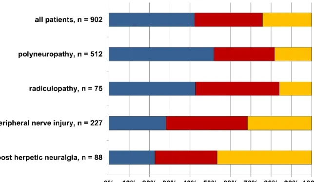
To analyze similarities between the mechanistic sensory subgroups described above and the sensory phenotypes found by hypothesis-free pattern searching methods in patients suffering from neuropathic pain, the patients suffering from neuropathic pain underwent the algorithm from 2.9 and the result was compared to each patient’s sensory phenotype as determined using the algorithm developed for patients in 2.7. Agreement between algorithms was assed using Cohen’s Kappa (Fleiss et al., 2003). We then applied a probabilistic sorting algorithm to estimate the prevalence of the three presumed mechanisms in this cohort of patients; this allows each patient to be assigned to more than one mechanism.
Results
3 RESULTS
3.1 Patients and participants
Patients and participants for the various analyses were not identical, and are therefore described briefly below.
3.1.1 Patients
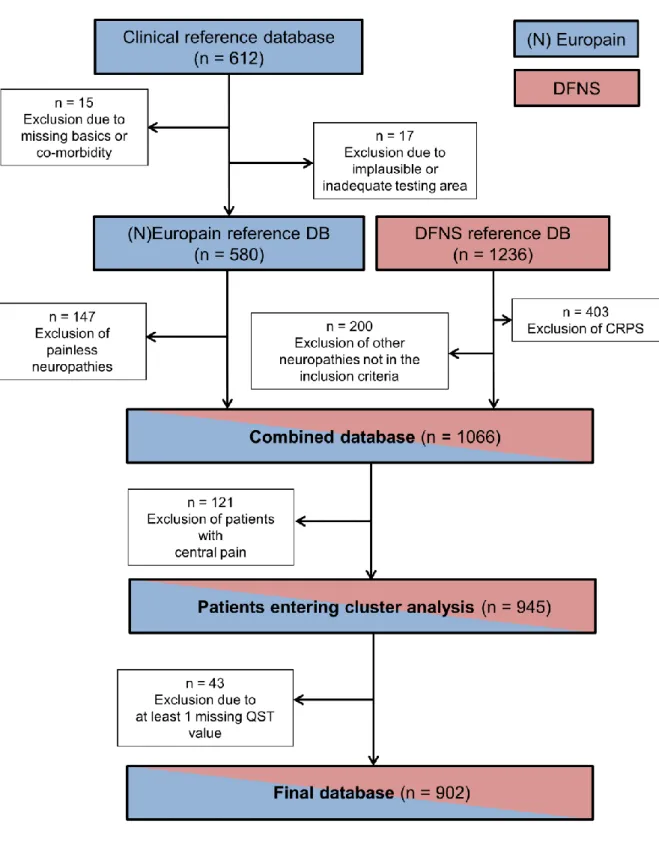
Essential basis of all analyses of patients was the European cohort, formed for the cluster analysis in patients (Baron et al., 2017). This cohort comprises n = 902 patients with peripheral neuropathic pain. Formation of this cohort is shown in Figure 1.
For the analysis of heterogeneity, a sub-collective of this cohort was formed: only data from centers which provided at least ten patients with painful polyneuropathy and ten patients with painful peripheral nerve injury were included. These ten centers provided 217 patients with painful PNP and 150 patients with painful PNI.
For the validation set of the cluster analysis in patients, a second cohort was formed from patients that were included by the DFNS after the closure of the initial database (Maier et al., 2010) and in the IMI for pharmacological studies (Demant et al., 2014; Demant et al., 2015). This group comprised n = 233 patients with peripheral neuropathic pain due to polyneuropathy, peripheral nerve injury or post-herpetic neuralgia.
For estimating frequency of phenotypes in etiologies of neuropathic pain and suggesting sample sizes for phenotype-stratified studies, the European cohort (n = 902) and the validation cohort (n = 233) were merged with data from the PiNS cohort (n = 209). From the resulting patient group, all patients with painful peripheral nerve injury (n = 335), painful diabetic polyneuropathy (n = 151), and painful post-herpetic neuralgia (n = 97) were extracted.
Results
Figure 1: CONSORT flowchart of data inclusion for the European cohort. CRPS: Complex Regional Pain Syndrome, DB: database. From (Baron et al., 2017).
Results
3.1.2 Healthy participants
For the analysis of heterogeneity and for separation of patients and healthy participants in the individual sorting algorithm, QST data from n = 188 healthy participants provided for ensuring quality control (Vollert et al., 2015) by ten European centers was included (Vollert et al., 2016a).
3.1.3 Human surrogate models
Many participants were tested more than once under various models, so the number of participants is less meaningful than the number of QSTs under surrogate models, which will therefore be referred to subsequently. A total of n = 657 QSTs under surrogate models could be included (see Table 1).
model n Gender:
n (%) female
Age:
mean (range) participating centers nerve block
A fiber block 24 12 (50%) 25 (21 - 39) Kiel, Mannheim
Topical lidocaine 41 20 (49%) 34 (19 - 69) Bochum
primary hyperalgesia
Topical capsaicin 273 147 (53%) 25 (15 - 75) Bochum, Frankfurt, Mannheim
UVB 158 51 (32%) 24 (19 - 42) Frankfurt, Mannheim
secondary hyperalgesia
Capsaicin injection 36 19 (53%) 32 (23 - 68) Kiel, Mannheim, Munich
Cutaneous HFS 12 3 (25%) 36 (24 - 57) Mannheim
mixed Topical capsaicin, secondary
hyperalgesia 37 15 (41%) 24 (19 - 39) Mannheim
UVB, secondary
hyperalgesia 22 0 (0%) 24 (24 - 24) Mannheim
Muscular HFS 15 7 (47%) 24 (19 - 27) Mannheim
Topical menthol 11 0 (0%) 25 (23 - 28) Kiel
Topical lidocaine + topical
Results
3.2 Analysis of heterogeneity
[The following section has been taken in parts and modified from (Vollert et al., 2016a).]
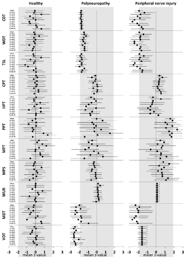
The forest plots for healthy participants, patients with polyneuropathy and peripheral nerve injury are shown in Figure 2 for each of the 11 normally distributed QST parameters, each of the 10 centers and mean effect. The forest plots show for each center, QST parameter and separately for healthy participants, PNP and PNI a center specific mean of each QST parameter, along with its 95% confidence interval. These confidence intervals indicate how individual and center-specific variance relate to each other: broader confidence intervals indicate high variance within centers that is not similar between all centers, narrow confidence intervals indicate high homogeneity within centers or variance that is similar between all centers.
Results
Figure 2: Forest plot of center-specific and overall mean QST z-values with 95% confidence intervals for healthy participants (left graph), patients with polyneuropathy (middle graph) and peripheral nerve injury (right graph). Note that confidence intervals are not equal to standard deviation or standard error
Results
3.2.1 Healthy participants
All center-specific mean z-values were found to be well within the normal range of 0 ± 1.96, the mean z-values per parameter are within 0 ± 0.20, with two exceptions: TSL (-0.26, 95% CI: -0.62; 0.10) and MPT (0.37, 95% CI: -0.01; 0.75). The overall mean z-value of all parameters and centers was found to be exactly 0.00. The 95% confidence intervals varied in width between 0.5 and 1.4, with a mean of 0.9. Broad confidence intervals indicate a high degree of individual variance within centers that is not found between all centers (i.e. the center-specific mean is uncertain). Inclusion of more participants per center might reduce the influence of this effect. In the given data, the largest part of variance is of individual origin, not between centers, which is represented in the I² values in Table 2 (first column), showing a heterogeneity of 0% for all parameters except PPT (41.8%, 95% CI: 0.0%; 66.1%) and MDT (5.4%, 95% CI: 0.0%; 18.1%).
Healthy participants Polyneuropathy Peripheral nerve injury CDT 0.0% (0.0% - 57.0%) 0.0% (0.0% - 0.0%) 0.0% (0.0% - 73.5%) WDT 0.0% (0.0% - 99.9%) 0.0% (0.0% - 54.0%) 0.0% (0.0% - 71.1%) TSL 0.0% (0.0% - 50.8%) 0.0% (0.0% - 57.9%) 0.0% (0.0% - 77.0%) CPT 0.0% (0.0% - 80.0%) 0.0% (0.0% - 91.1%) 0.0% (0.0% - 50.6%) HPT 0.0% (0.0% - 100.0%) 0.0% (0.0% - 98.9%) 0.0% (0.0% - 79.0%) PPT 41.8% (0.0% - 66.1%) 0.0% (0.0% - 82.3%) 0.0% (0.0% - 58.2%) MPT 0.0% (0.0% - 76.5%) 0.0% (0.0% - 99.8%) 0.0% (0.0% - 76.8%) MPS 0.0% (0.0% - 100.0%) 0.0% (0.0% - 59.3%) 0.0% (0.0% - 69.2%) WUR 0.0% (0.0% - 45.3%) 0.0% (0.0% - 33.5%) 0.0% (0.0% - 0.0%) MDT 5.4% (0.0% - 18.1%) 0.0% (0.0% - 92.1%) 0.0% (0.0% - 56.4%) VDT 0.0% (0.0% - 89.1%) 0.0% (0.0% - 26.7%) 0.0% (0.0% - 0.0%)
Table 2: I² Index of heterogeneity, ranging from 0% (no heterogeneity) to 100% (perfect heterogeneity) for all eleven normally distributed QST parameters for healthy participants (n = 188), polyneuropathy patients (n = 217) and patients with peripheral nerve injury (n = 150). In brackets: lower and upper boundary of the 95% confidence interval. All values except PPT and MDT in healthy participants are zero, though the confidence intervals often cover a broad range up to 100% due to the broad confidence intervals of center specific mean z-values. From (Vollert et al., 2016a).
Results
3.2.2 Polyneuropathy
Center specific mean z-values for detection thresholds were characterized by loss of thermal and mechanical detection (CDT, WDT, TSL, MDT, VDT), which is typical for patients suffering from polyneuropathy. Note that the small confidence intervals (esp. for cold and warm detection threshold) do not reflect little variation in the dataset, but rather that only a small part of this variation is assigned to the center, the remainder is assigned to individual effects (ɛ𝑖𝑗 in F(1)) that appear across centers in similar form. For pain thresholds, ranges of center specific mean z-values and confidence intervals were found to be much broader, especially for MPT and PPT. Mean z-values scattered within the normal range of 0 ± 1.96, but very broad confidence intervals show that this indicates merely high individual variance between PNP patients rather than systematic deviation by single centers. This is represented in I² values indicating heterogeneity of 0% between the centers for all parameters (Table 2, middle column).
3.2.3 Peripheral nerve injury
Similar as for PNP, center specific mean z-values for detection thresholds in PNI patients showed loss of function. Pain thresholds are mainly decreased (with HPT as exception), as expected for PNI patients, who often show a combination of loss of detection and gain of nociception. Confidence intervals are broader compared to PNP, indicating that a larger amount of variance is found within instead of between centers. For wind-up ratio and vibration detection threshold, individual variation was found to superimpose any possible center specific effects (𝑎𝑖 in F(1)) in patients suffering from PNI, so the forest plot (Figure 2, right column) presents only the overall mean and its confidence interval instead of center specific means for all centers (𝜇
instead of 𝜇 + 𝑎𝑖). As almost all center specific mean z-values lie within the confidence intervals of each other, the I² index of heterogeneity is 0% for all parameters.
Results
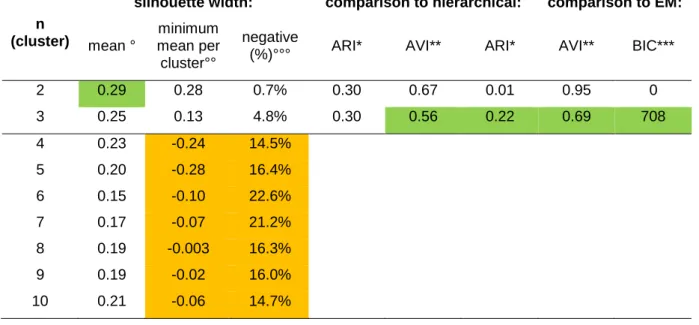
According to the frequency of negative silhouette widths we excluded the solutions with 4 - 10 clusters because they each presented at least one cluster with a negative mean silhouette width that indicated an artifact. Furthermore, in each of these solutions negative silhouettes were frequent (15 - 23%). The remaining two and three cluster solutions were compared with two additional, mathematically different clustering algorithms for the same number of clusters. Compared with agglomerative hierarchical cluster analysis, both 2 and 3-cluster solutions were equal according to the ARI criterion, but the three-cluster solution was better according to the AVI criterion. In comparison to the EM algorithm, the two-cluster solution failed to show similarity between k-means and EM clustering (ARI almost zero, AVI almost 1). Since the Delta-BIC also strongly preferred the cluster solution (Table 3), the three-cluster solution was used for further analysis as the optimal number of three-clusters. The replication data set was also subjected to a k-means cluster analysis with k = 3.
Results
n (cluster)
silhouette width: comparison to hierarchical: comparison to EM: mean °
minimum mean per cluster°°
negative
(%)°°° ARI* AVI** ARI* AVI** BIC***
2 0.29 0.28 0.7% 0.30 0.67 0.01 0.95 0 3 0.25 0.13 4.8% 0.30 0.56 0.22 0.69 708 4 0.23 -0.24 14.5% 5 0.20 -0.28 16.4% 6 0.15 -0.10 22.6% 7 0.17 -0.07 21.2% 8 0.19 -0.003 16.3% 9 0.19 -0.02 16.0% 10 0.21 -0.06 14.7%
Table 3: Decision on the number of clusters. Green: optimum number of clusters according to this criterion. °Mean silhouette width per cluster. A value below zero indicates clusters that do not separate from other clusters. Measure of discriminatory power (0 to 1). 0: no discrimination, 1: perfectly separated clusters (high values are preferred) °°Measure of fragmentation of solution (-1 to +1). -1: cluster that is solely a fragment, +1: a solution that is not fragmented (solutions with values below zero were discarded (yellow)) °°°Measure of fragmentation of solution (0% to 100%). 0%: no fragmentation, 100% a completely fragmented solution (solutions with values above 10% were discarded (yellow)) *ARI (Adjusted Rand Index): Measure of similarity (0 to 1). 0: only random identity, 1: perfect identity (high values are preferred) **AVI (Adjusted Variation of Information): Measure of dissimilarity (0 to 1). 0: no dissimilarity, 1: strong dissimilarity (low values are preferred) ***Delta-BIC (Bayesian Information Criterion): Measure of gain of information by increasing cluster number. If delta-BIC > 10, the higher cluster number is recommended. Modified from (Baron et al., 2017).
3.3.1 Sensory profiles of the three-cluster solution
Figure 3 shows the mean z-score sensory profiles for the test data set (Fig. 3A) and the validation data set (Fig. 3B). In both data sets, the clusters represented similar percentages of patients: cluster 1 was the largest (42% in A, 53% in B), followed by cluster 2 (33% in A and B) and cluster 3 (24% in A, 14% in B). Sensory profiles were also replicated excellently. For non-nociceptive temperature sensation (CDT, WDT, TSL), clusters 1 and 3 exhibited pronounced deficits with mean z-scores near -2, while temperature sensation was essentially normal in cluster 1. This offset was similar for thermal pain sensitivity (CPT, HPT), but here clusters 1 and 3 exhibited
Results
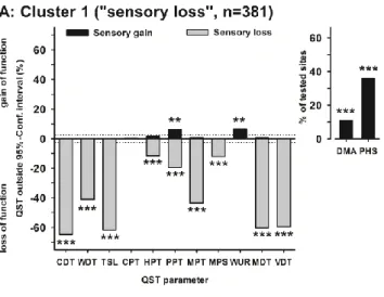
(PPT, MPT, MPS), the rank order between clusters was different and cluster 1 and 3 were separated: while there was again a deficit for cluster 1, cluster 3 exhibited significant sensory gain. Cluster 3 was therefore given the label "mechanical hyperalgesia". Wind-up did not differentiate between clusters. For non-nociceptive touch sensation (MDT, VDT), cluster 2 was again close to normal, cluster 3 had some deficit, and cluster 1 exhibited the most pronounced deficit. Cluster 1 was given the label "sensory loss", because it was characterized by negative mean z-scores across all QST parameters. Dynamic mechanical allodynia (DMA) was most pronounced in cluster 3, which also exhibits the most pronounced hyperalgesia to pinprick (MPT, MPS) and blunt pressure (PPT). Paradoxical heat sensations were most pronounced in cluster 1, associated with diminished cold detection (CDT) but not cold hyperalgesia (CPT).
Figure 3: Sensory profiles of the three-cluster solution for test and replication data sets. Sensory profiles of the three clusters presented as mean z scores ± 95% confidence interval for the test dataset (n = 902, A) and the validation dataset (n = 233, B). Note that z-transformation eliminates differences due to test site, gender and age. Positive z-scores indicate positive sensory signs (hyperalgesia), negative z-values indicate negative sensory signs (hypoesthesia, hypoalgesia). Dashed lines: 95% confidence interval for healthy participants (-1·96 < z < +1·96). Inserts show numeric pain ratings for DMA on a logarithmic scale (0-100) and frequency of PHS (0-3). Blue symbols: cluster 1 "sensory loss" (42% in A, 53% in B). Red symbols: cluster 2 "thermal hyperalgesia" (33% in A and B). Yellow symbols: cluster 3 "mechanical hyperalgesia" (24% in A, 14% in B). From (Baron et al., 2017).
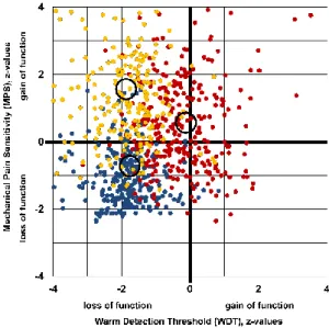
Figure 4 illustrates the distinction of the three clusters in a 2D-scatter-plot and histograms of those two QST parameters that exhibited the best separation of
Results
clusters: warm detection threshold (WDT) and mechanical pain sensitivity (MPS). Patients in cluster 1 had loss of pinprick sensitivity, while those in cluster 3 had pinprick hyperalgesia. Most patients in cluster 2 had WDT within the normal range of ±1.96 z-values, while many of clusters 1 and 3 had hypoesthesia to warmth (z-values below -1.96). Although the k-means cluster separation was calculated in 13-dimensional space, this 2D-projection illustrates some of the main characteristics how the three clusters differ between each other. Partial overlap between clusters may also be due to two mechanisms present in the same patient. WDT and MPS were therefore chosen for simplified phenotyping subsequently.
Figure 4: Cluster separation projected onto two-dimensional space. Histograms and scatter plot of the two QST-parameters that gave the best cluster separation: warm detection threshold (WDT) and mechanical pain sensitivity (MPS). Blue: cluster 1 "sensory loss" (n=381 patients), red: cluster 2 "thermal hyperalgesia" (n=302 patients), yellow: cluster 3 "mechanical hyperalgesia" (n=219 patients). Circles indicate centroids of each cluster. Modified from (Baron et al., 2017).
3.3.2 Patient characteristics of the three clusters
The patients´ gender and mean age as well as pain intensity did not differ between the three groups (Table 4). Depressive symptoms occurred significantly more frequently in the “sensory loss” cluster. Spontaneous pain described by the patients