Improving learning vector quantization using data
reduction
Pande Nyoman Ariyuda Semadi a,1, Reza Pulungan a,2,*
a Department of Computer Science and Electronics, Faculty of Mathematics and Natural Sciences,
Universitas Gadjah Mada, Yogyakarta, Indonesia
1[email protected]; 2 [email protected]
* corresponding author
1.
Introduction
Learning Vector Quantization (LVQ), developed by Kohonen, is a supervised learning algorithm and is specialized for statistical classification and pattern recognition [1]. LVQ aims at determining section areas of each class of the input data. This algorithm has been widely used in various fields, such as for phoneme [2] and character recognition [3][4], fingerprint verification [5][6], object orientation detection [7], intrusion detection [8], classification of woven fabric structure [9], variables ordering [10], driving pattern recognition [11], cognitive skill classification [12], textual document classification [13], time series prediction [14], classification of computer network attacks [15], and for improving hierarchical neural networks [16].
Some initial values in LVQ must be defined before the learning process begins. Furthermore, one of the essential parameters in establishing a good classification model is the reference vectors. LVQ is sensitive to its reference vector initialization because it will affect its convergence [17]. Random weight initialization selection frequently is not accurate enough [18]. A procedure to determine better initial reference vectors or weights is therefore required for the optimal running of the LVQ network; one of them is through clustering, as suggested by Vakil-Bagmisheh and Pavešić [19].
Data reduction is one of many ways developed to reduce the amount of data that must be stored by instance-based algorithms. Deleting some data points from the learning dataset often significantly accelerates the classification model to achieve the expected condition. Data reduction is carried out by still maintaining the existing accuracy. In some cases, the removal of data considered as the noise could even increase the model’s accuracy [20]. Data reduction method can be developed by reviewing various A R T I C L E I N F O A B S T R A C T
Article history
Received February 3, 2019 Revised October 31, 2019 Accepted November 22, 2019 Available online November 22, 2019
Learning Vector Quantization (LVQ) is a supervised learning algorithm commonly used for statistical classification and pattern recognition. The competitive layer in LVQ studies the input vectors and classifies them into the correct classes. The amount of data involved in the learning process can be reduced by using data reduction methods. In this paper, we propose a data reduction method that uses geometrical proximity of the data. The basic idea is to drop sets of data that have many similarities and keep one representation for each set. By certain adjustments, the data reduction methods can decrease the amount of data involved in the learning process while still maintain the existing accuracy. The amount of data involved in the learning process can be reduced down to 33.22% for the abalone dataset and 55.02% for the bank marketing dataset, respectively.
This is an open access article under the CC–BY-SA license.
Keywords
Learning vector quantization Data reduction
Geometric proximity Euclidean distance
approaches so that differences, as well as similarities among data, can be determined. One of the existing data reduction methods is based on establishing subsets of the data. This subset-based data reduction method is affected by the distribution of the data. The development of various methods of data reduction is feasible because of the proliferation of ideas and approaches that can be carried out to achieve them. Data reduction is different from feature selection, which deletes non-essential features, namely dimension, in high dimensional data [21].
The development of ideas for optimization has been running for decades. In the early days, LVQ was optimized by attempting to improve its convergence. Kitajima in [17] was concerned with the relationship between the convergence of reference vectors and the performance of the network. The idea is to place the reference vectors as close as possible to the approximate stable position. The placement of reference vectors can be adjusted according to area density in the data. For this purpose, the research used properties of the self-organizing map classification algorithm to determine the position of the reference vectors in order that the position matches the distribution of the data.
The idea of data reduction in classification algorithms begins with the research of Wilson and Martinez [20][22]. Their study provided an overview of some criteria of data-based algorithms, which include distance function, data representation, and general intuition in maintaining data. They conducted research to devise a data reduction method that is capable of reducing the amount of data significantly without drastically reducing the classification accuracy. This data reduction method was then applied to the nearest neighbor algorithm. The approach presented by Wilson and Martinez forms the basis for our current proposed method for a similar implementation on LVQ.
Vakil-Bagmisheh and Pavešić [19] originally studied premature clustering, a condition when changes in the central cluster are only due to oscillations. This study also recommended the implementation of clustering at the beginning of the LVQ training algorithm and used the cluster center generated as initial vector values. This is due to the sensitivity of LVQ associated with the initial values of the reference vectors. Their results support Kitajima’s [17]. Pedreira [23] stated that the success of a classification scheme could be linked to data processing accuracy. They attempted to perform data selection so that the network can be directed to achieve convergence at a better location. This research resulted in a better error level when compared to the usual LVQ.
Lv et al. in [4] introduced a method that provides additional vectors for every selected reference vector. The additional vector, which is called the importance vector, has the same structure and is renewed just like a reference vector. The experimental result showed that the performance of LVQ that has been modified with this procedure could overtake the standard LVQ in terms of data adaptation.
In their research, Blachnik and Duch [18] stated that every model of artificial neural network needs a proper network parameter initialization to produce an optimal classification model. This research carried out data selections using the rules of similarities of inter-intraclass and edited nearest neighbor. This method succeeded in simplifying the classification model without losing its accuracy. The edited nearest neighbor itself is a method developed by Wilson and Martinez [20].
Chou et al. in [24] made another improvement on nearest-neighbor-based data reduction and proposed generalized condensed nearest neighbor. The method can outperform the original condensed nearest neighbor and give more consistent results under certain conditions. Wang et al. [25] used a data reduction technique to identify the essential key features instead of just reducing the numbers of data. The method can also determine the optimal number of clusters by deleting noisy data and enhancing the distance between different clusters. Ougiaroglou et al. [26] proposed a data reduction technique based on the k-median clustering algorithm. The idea is to balance the trade-off between speed and performance: how to speed up the algorithm with minimum or no sacrifice in performance. The research showed that performance degradation in support vector machines is less than in neural networks.
This paper proposes a data reduction method based on geometric proximity among data in a dataset. The data reduction method is applied before LVQ training to reduce the size of data but still maintain its accuracy. After the data reduction process is carried out, there will be a set of data with a smaller size but has a representation close to the initial dataset.
The rest of the paper is organized as follows: Section 2 discusses methods related to LVQ, general data reduction, and the proposed data reduction. In Section 3, we present experiments that we have conducted and provide analysis. Section 4 concludes the paper.
2.
Method
2.1.Learning vector quantization
Artificial neural networks (ANN) are information processing systems with certain procedural characteristics that resemble biological neural networks [27]. Artificial neural networks are designed as artificial representations by simulating the learning processes that occur in the human brain and are created with computer programs. Based on the characteristics of the mechanisms performed, a learning process can be classified into a supervised or unsupervised learning process [27].
LVQ was initially introduced as a tool in image compression before it was then adopted and adapted by Kohonen as an algorithm for pattern recognition [27]. LVQ is a learning procedure on a supervised competitive layer. The competitive layer automatically learns to classify the input vectors based on distance calculation. LVQ network architecture consists of only input and output layers, which makes it relatively faster [28] and less time consuming than other ANN, such as multilayer perceptron [29].
A weight vector of LVQ, often referred to as a reference vector or a codebook, represents a particular class or category. Each class can be represented by one or more output units, in which each output unit is associated with a specified target class [30]. During the training process, the position of a reference vector will be adjusted by changing the values of its components. If the reference vector is in the same class as the input vector, its position will be brought closer. On the contrary, the reference vector will be kept away from the position of the input vector if they reside in different classes. The final result of LVQ training is a collection of vectors that can serve as references for classifying an input unit. If two input vectors are close together, then it will be mapped into the same class by the competitive layer
[27].
Let T(x) be the class of input vector x, C(w) be the class of the output unit associated with reference vector w, and n be the number of reference vectors. The procedure of LVQ is as follows [23]:
1) Initialize the set of reference vectors {wi | i = 1, · · ·, n} and the learning rate α.
2) While the stopping condition is not fulfilled, do steps 2–7. 3) For each training input vector x, do steps 3–4.
4) Find a reference vector w such that ∥x − w∥ is minimum. 5) Update w as follows:
(1) 6) Reduce the learning rate α.
7) Check whether the stopping condition is fulfilled.
The stopping condition may be specified as a fixed number of iterations or when the learning rate reaches a predefined threshold.
2.2.Data reduction
Several issues are faced in classification: class imbalance, the number of features and the size of data to be stored. Class imbalance occurs when instances distribution among classes differs much [31]. This condition affects the accuracy and decrease the effectiveness of the classification techniques [32]. High dimensional data occurs when data has too many features; sometimes up to hundreds or thousands features. This condition affects the computation workload and procedures to delete non-essential features are needed [21]. Feature deletion, however, must pay attention to feature measurement by
carrying out some evaluation [33]. Another common problem is the growth of data, in which data reduction becomes an important issue in the field of data mining [34].
A data reduction method was developed to provide solutions to problems commonly encountered by instance-based algorithms, namely determining which data points need to be stored. Storing too much data can cause excessive sensitivity to noise as well as slowing down execution speed [20]. There is no specific algorithm to carry out the data reduction process, and various factors must be taken into consideration when developing a data reduction method. Wilson and Martinez [20] presented several crucial issues that must be addressed in the development of data reduction techniques, as follows: 1) Representation. One approach in designing the data reduction method is to decide whether to retain
a subset of the original instances or to modify the instances using a new representation.
2) The direction of search. This issue is about various usable schemes to create subsets of training data, such as incremental, decremental, and batch. Forming a subset by an incremental search means initiating the formation of an empty subset and then entering each data point that meets the criteria into that subset. Decremental search does the opposite, with the initial condition of all data points being subset members and then deleting data points by applying specific rules. Batch search combines both.
3) Border points vs. central points. This issue concerns evaluating and deciding which data points to retain; border points, central points, or some other set of points. Some algorithms retain the border points because internal points do not affect the decision boundaries as much as border points, and thus can be removed with relatively little effect on the classification. On the other hand, some algorithms remove the border points because they are considered as noise.
4) Distance function. The distance function commonly used in the nearest-neighbor algorithm and its derivatives is the Euclidean function. Application of different distance functions, such as Manhattan or Canberra, can give different results. Some algorithms use weighting schemes as an alternative to distance measurements and the voting influence of each instance.
5) Voting. The voting concept is often taken into consideration in maintaining or reducing data. A data point is compared to several other k units of the nearest data and evaluated for their corresponding classes.
6) Evaluation strategies. An evaluation strategy is concerned with the benefits that a data reduction technique will provide because each data reduction technique has advantages and disadvantages. Factors to be considered in the evaluation include storage reduction, speed increase, generalized accuracy, noise tolerance, learning speed, and the possibility of adding data at any time.
2.3.Proposed data reduction method
Data reduction is based on the idea that in a collection of learning data, there exist some insignificant data points that do not determine the classification process. This is due to the proximity of the distance to other data in the same class. If the insignificant data points are deleted, the classification result is not affected. With a systematic simplification method, there will be a set of data that has a smaller size but has a representation close to the initial dataset.
The data reduction process is carried out internally for each class. Our proposed data reduction algorithm, an improvement of the algorithm proposed in [35], is as follows:
1) For each class, determine the center point of the class. The center point is a point that is geometrically located in the middle. Each vector element of the center point is the average of the corresponding vector element of all data points. Let xi, for 1 ≤ i ≤ n, be the vectors representing the m-dimensional
data points in the class, then xt, namely the vector representing the center point of the class, is defined
(2) 2) Calculate the radius of the class by:
(3) where R is the radius, and k is a radius coefficient ranging from 0 to 1. In this research, the term radius is used for the average Euclidean distance from each data point to the class’ center point. For two data points 𝒙1 and 𝒙2, their Euclidean distance is defined by [22]:
(4) 3) Determine the relationship of each data point by comparing its distance to other data points with its
radius.
4) Select the data point that has the largest number of other data points within its radius to represent the set of data points. This data point is called a candidate.
5) Delete all other data points that are within the radius of the candidate.
6) Perform steps 5 and 6 for the next data point with the largest number of other data points within its radius.
7) Reduction is completed when no two data points are within each other’s radius.
The result of the data reduction process is a number of data points selected as representatives of all other data points within their scope. The selection process and the number of removed data points are influenced by the geometric location and the distribution of the data. The radius coefficient k can be used to determine the range of the radius. The longer the radius, the more data points will be removed, and the distance among the candidates will be longer. Fig. 1(a) to 1(e) show how the data reduction method is carried out.
(a) (b) (c)
(d) (e)
Fig. 1(a) depicts the initial state. Data points a, b, c, d, e, f, g, h, i, and j are members of one class, while data points k, l, and m are members of another class. Fig. 1(b) shows the center point for each class, represented by the plus (+) signs. Fig. 1(c) illustrates the process of calculating the distance from each data point to the center point and then calculating the average for each class. Fig. 1(d) shows the radius range of each data point, represented by the circles. As described before, the radius is calculated by multiplying the average distance with the coefficient k. Fig. 1(e) depicts a new dataset consisting of every candidate selected. The figure indicates that data points a and c in the first class are deleted because they are in the radius coverage of data point b, while data point b has been selected as a candidate. The same thing happens to data points e and g. However, there is no data point deleted in the second class, since no data point is located within another's radius.
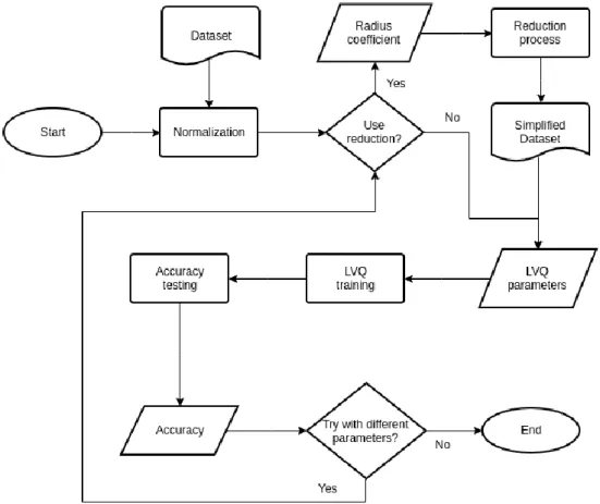
Fig. 2 depicts the flowchart of the proposed method. As previously described, the data reduction method is carried out as optional preprocessing steps before LVQ training. In the beginning, all data points in the dataset are normalized before the data reduction method is applied. For the data reduction method, the user must provide the radius coefficient, which determines the granularity of the data reduction. Once the data reduction method is completed, the user determines the LVQ parameters, such as the learning rate, the number of vector references, and the maximal iteration. The geometrical-based data reduction method will reduce the number of data points in the dataset. Outputs of these preprocessing steps are a smaller sized dataset, which will become inputs to LVQ training. Once LVQ training is completed, its accuracy is then evaluated.
Fig. 2.Flowchart of the proposed method
3.
Results and Discussion
This section details the experimental setting as well as the results of the experiments we have conducted to evaluate the proposed method. In the evaluation, two standard benchmark datasets are used, namely abalone and bank marketing. The abalone dataset consists of 2 classes, 4177 data points, each with 11 attributes after nominal-to-binary conversion. The bank marketing dataset consists of 2 classes, 4521 data points, each possessing 49 attributes after nominal-to-binary conversion.
In the evaluation, two series of experiments are conducted for each dataset by varying the radius coefficient from 0.0, 0.01, 0.02, until 0.1 for the abalone dataset and from 0.0, 0.1, 0.2, until 1.0 for the bank marketing dataset. The abalone dataset is more sensitive to the radius coefficient, so the coefficient applied is smaller. In the first series of experiments, the data reduction method is applied before LVQ training, while in the second, the data reduction method is applied to other classification methods, namely self-organizing map (SOM), decision tree J48, and backpropagation, to compare their testing accuracy.
Two measures will be collected and computed from these series of experiments, namely accuracy and training time. Accuracy refers to the training as well as testing phases of LVQ on each dataset, while the training time refers to the time it takes to run the LVQ training process. For each value of the radius coefficient, five LVQ training processes are run. For the training time, the average value, as well as the corresponding standard deviation, will be collected.
Table 1 and Table 2 show the results of the series of experiments for abalone and bank marketing datasets, respectively. Each table comprises five columns, listing the radius coefficient used, the percentage of the remaining data from the original dataset once the data reduction process is applied, the training and testing accuracy in percentage, and the mean LVQ training time and its standard deviation in milliseconds. Even though the LVQ training is performed using the reduced training dataset, the training accuracy is measured using the original training dataset.
Table 1. Results of applying the data reduction method on the abalone dataset Radius coefficient % Data remaining Training accuracy (%) Testing accuracy (%) LVQ training time Mean (ms) Stdev 0 100 77.55 75.96 20.6 2.70 0.01 99.57 77.55 75.91 20.6 3.58 0.02 93.63 77.93 76.15 19.0 3.39 0.03 82.77 77.93 77.25 18.6 3.05 0.04 71.61 78.08 76.10 18.0 3.46 0.05 56.58 76.64 74.90 17.6 2.30 0.06 43.71 77.60 76.01 16.8 2.77 0.07 33.22 76.64 75.72 16.4 2.61 0.08 26.76 75.39 73.90 15.8 0.84 0.09 21.69 75.20 72.13 15.4 0.89 0.1 18.24 75.11 70.59 14.4 1.52
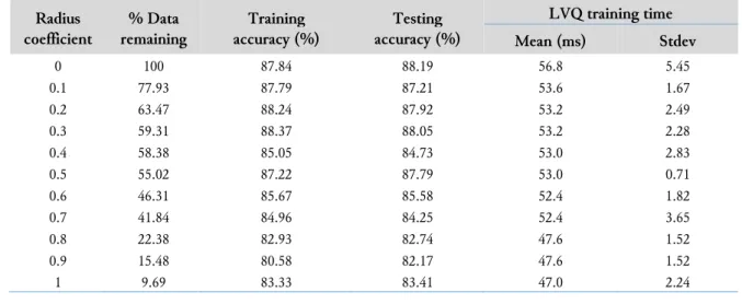
Table 2. Results of applying the data reduction method on the bank marketing dataset Radius coefficient % Data remaining Training accuracy (%) Testing accuracy (%) LVQ training time Mean (ms) Stdev 0 100 87.84 88.19 56.8 5.45 0.1 77.93 87.79 87.21 53.6 1.67 0.2 63.47 88.24 87.92 53.2 2.49 0.3 59.31 88.37 88.05 53.2 2.28 0.4 58.38 85.05 84.73 53.0 2.83 0.5 55.02 87.22 87.79 53.0 0.71 0.6 46.31 85.67 85.58 52.4 1.82 0.7 41.84 84.96 84.25 52.4 3.65 0.8 22.38 82.93 82.74 47.6 1.52 0.9 15.48 80.58 82.17 47.6 1.52 1 9.69 83.33 83.41 47.0 2.24
3.1.Trade-off between storage and accuracy
Before applying the preprocessing, we perform preliminary experiments to measure the accuracy of the standard implementation of LVQ. The training accuracy of abalone and bank marketing datasets is 77.5491% and 87.8372%, respectively, while the testing accuracy of abalone and bank marketing datasets is 75.9579% and 88.1858%, respectively. These values correspond to the first row of each table. LVQ parameters used in this experiment are learning rate 0.1, 50 randomly generated proportional reference vectors, and maximum iteration 10000.
The evaluation of the data reduction method indicates that the accuracy of LVQ can be maintained close to the original one with less amount of training data. The critical value of the radius coefficient— namely, a value once exceeded results in an accuracy that is no longer considered viable—differs for each dataset. The critical value of the radius coefficient is 0.07 for the abalone dataset and 0.5 for the bank marketing dataset. The advantages enjoyed by each dataset are as follow:
1) When the radius coefficient is 0.07 in the abalone dataset, the remaining data is only 33.22% or, in other words, a saving of 66.78% of the storage. The classification accuracy in this case only decreases 0.9096% for the training data and 0.2395% for the testing data. The LVQ training time also gets reduced and only needs 79.61% of the time required by the standard training dataset.
2) When the radius coefficient is 0.5 in the bank marketing dataset, the remaining data is only 55.02%, namely, a saving of 44.98% of the storage. The classification accuracy in this case only decreases 0.6192% for the training data and 0.3982% for the testing data. The LVQ training time also decreases to 93.3% of the time needed by the standard training dataset.
For the two datasets, it is evident that the data reduction method achieves a significant reduction of data (all manage a reduction of more than 40% of the original size) while only sacrificing little accuracy. It should also be noted that data reduction may sometimes result in even better accuracy, as seen on the abalone dataset, despite the smaller set of data used in training. Previous research [20] suggested that this may be because data reduction manages to eliminate noises in the dataset. In our experiments, improvements in the accuracy occur when the radius coefficient is 0.02 until 0.04 for the abalone dataset.
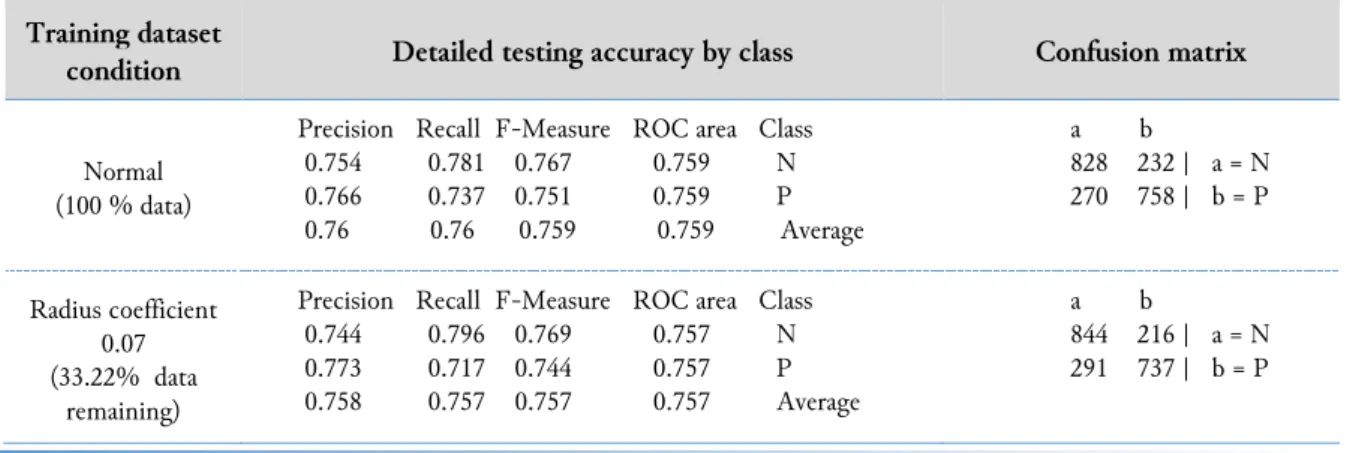
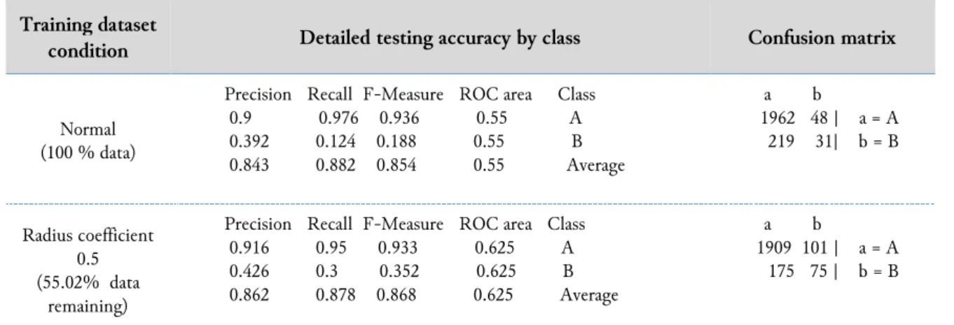
Table 3 and Table 4 show the details of the testing accuracy for both datasets. Inspecting Table 3, we can observe that both the average F-measure and the average receiver operating characteristics (ROC) area, when data is 100% and when the radius coefficient is critical, are not significantly different. This implies that the accuracy and threshold before and after applying the data reduction in the abalone dataset are similar. From Table 4, on the other hand, we can observe that, in the bank marketing dataset, when the radius coefficient is critical—namely, when the data reduction is in full capacity—the increase in the average F-measure and the average ROC area is more significant. This means that data reduction has more impact on this dataset. Furthermore, from the confusion matrix, we can observe that a better classification result is produced for class B. A better ROC value indicates that the model is better in discriminating classes A and B. Note that the class distribution in the bank marketing dataset is unbalanced.
Table 3. Detailed testing accuracy of the abalone dataset when the radius coefficient is critical Training dataset
condition Detailed testing accuracy by class Confusion matrix
Normal (100 % data)
Precision Recall F-Measure ROC area Class 0.754 0.781 0.767 0.759 N 0.766 0.737 0.751 0.759 P 0.76 0.76 0.759 0.759 Average a b 828 232 | a = N 270 758 | b = P Radius coefficient 0.07 (33.22% data remaining)
Precision Recall F-Measure ROC area Class 0.744 0.796 0.769 0.757 N 0.773 0.717 0.744 0.757 P 0.758 0.757 0.757 0.757 Average a b 844 216 | a = N 291 737 | b = P
Table 4. Detailed testing accuracy of the bank marketing dataset when the radius coefficient is critical Training dataset
condition Detailed testing accuracy by class Confusion matrix
Normal (100 % data)
Precision Recall F-Measure ROC area Class 0.9 0.976 0.936 0.55 A 0.392 0.124 0.188 0.55 B 0.843 0.882 0.854 0.55 Average a b 1962 48 | a = A 219 31| b = B Radius coefficient 0.5 (55.02% data remaining)
Precision Recall F-Measure ROC area Class 0.916 0.95 0.933 0.625 A 0.426 0.3 0.352 0.625 B 0.862 0.878 0.868 0.625 Average a b 1909 101 | a = A 175 75 | b = B
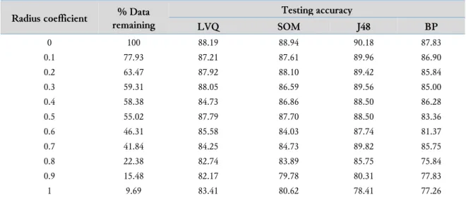
3.2.Testing accuracy comparison with other classification algorithms
Another series of experiments are carried out to investigate the influence of the data reduction method on the testing accuracy of LVQ compared with other classifier algorithms, namely SOM, J48, and backpropagation, on the two datasets. Table 5 shows the parameters used for the classification algorithms. Table 6 and Table 7 depict the testing accuracies of the four classifier algorithms for abalone and bank marketing datasets for various radius coefficients.
Table 5. Parameters of each classification algorithm Learning vector
quantization Self-organizing map Decision tree J48 Backpropagation
Learning rate: 0.1,
maximum training iterations: 10000,
total codebook: 50.
Learning rate; 0.1,
maximum training iterations: 10000.
Confidence factor: 0.1, unpruned: false,
minimum object per leaf: 2.
Learning rate: 0.1, hidden nodes: 5, maximum epoch: 1000.
Table 6. Testing accuracy comparison for the abalone dataset
Radius coefficient % Data remaining Testing accuracy LVQ SOM J48 BP 0 100 75.96 73.47 77.39 78.93 0.01 99.57 75.91 72.89 77.39 79.69 0.02 93.63 76.15 73.28 77.39 79.17 0.03 82.77 77.25 71.98 77.35 78.93 0.04 71.61 76.10 72.89 76.77 79.89 0.05 56.58 74.90 72.46 71.70 78.30 0.06 43.71 76.01 71.36 71.89 78.35 0.07 33.22 75.72 70.11 72.61 76.48 0.08 26.76 73.90 72.51 75.10 74.28 0.09 21.69 72.13 69.64 71.26 77.83 0.1 18.24 70.59 69.35 71.89 78.83
Table 7. Testing accuracy comparison for the bank marketing dataset Radius coefficient % Data
remaining Testing accuracy LVQ SOM J48 BP 0 100 88.19 88.94 90.18 87.83 0.1 77.93 87.21 87.61 89.96 86.90 0.2 63.47 87.92 88.10 89.42 85.84 0.3 59.31 88.05 86.59 89.56 85.00 0.4 58.38 84.73 86.86 88.50 86.28 0.5 55.02 87.79 87.70 88.50 83.36 0.6 46.31 85.58 84.03 87.74 81.37 0.7 41.84 84.25 84.73 89.82 85.75 0.8 22.38 82.74 83.89 85.75 75.84 0.9 15.48 82.17 79.78 80.31 77.83 1 9.69 83.41 80.62 78.41 77.26
From both tables, we can observe that LVQ is slightly better than SOM in retaining accuracy because SOM experiences a more significant decrease in accuracy for larger radius coefficients. In J48, the critical value of the radius coefficient is smaller, which means that only a smaller amount of data can be reduced when a similar accuracy is maintained. A unique pattern occurs in experiments using the backpropagation algorithm. For the abalone dataset, the accuracy of the backpropagation algorithm is good for almost every condition. A different result happens for the bank marketing dataset, though, namely, a decrease in accuracy even more severe than LVQ.
4.
Conclusion
In this paper, we have proposed a preprocessing method to improve the LVQ training in terms of storage and computation time. The proposed method indeed improves the training time of LVQ without a significant decrease in training and testing accuracy. In some cases, the reduction may even increase the training accuracy. Furthermore, a viable accuracy can still be achieved when the radius coefficient is 0.07 for the abalone dataset and 0.5 for the bank marketing dataset. At these values of the radius coefficient, there are only 33.22% and 55.02% data left in abalone and bank marketing datasets, respectively. This is a significant reduction of data for a still-acceptable level of accuracy. In principle, the data reduction method is orthogonal to the LVQ algorithm. The method is general, which can be applied as general preprocessing steps in any vector-based classification or pattern recognition algorithm. Researches on applying the data reduction methods on other learning algorithms are worth pursuing. We also plan to try to shorten the computation times of the data reduction method to improve the training time of the learning algorithms further.
References
[1] T. Kohonen, Self-Organizing Maps, 2001, vol. 30, doi: 10.1007/978-3-642-56927-2.
[2] K. M. O. Nahar, M. Abu Shquier, W. G. Al-Khatib, H. Al-Muhtaseb, and M. Elshafei, “Arabic phonemes recognition using hybrid LVQ/HMM model for continuous speech recognition,” Int. J. Speech Technol., vol. 19, no. 3, pp. 495–508, Sep. 2016, doi: 10.1007/s10772-016-9337-5.
[3] F. Camastra, “Handwritten Greek Character Recognition with Learning Vector Quantization,” in: Apolloni B., Howlett R.J., Jain L. (eds) International Conference on Knowledge-Based and Intelligent Information and
Engineering Systems (KES 2007), Lecture Notes in Computer Science, vol. 4694, pp. 267–274, doi:
10.1007/978-3-540-74829-8_33.
[4] Chuanfeng Lv, Xing An, Zhiwen Liu, and Qiangfu Zhao, “Dual Weight Learning Vector Quantization,” in
2008 9th International Conference on Signal Processing, 2008, pp. 1722–1725, doi:
[5] J. C. Yang, S. Yoon, and D. S. Park, “Applying Learning Vector Quantization Neural Network for Fingerprint Matching,” in: Sattar A., Kang B. (eds) Australasian Joint Conference on Artificial Intelligence (AI
2006), Lecture Notes in Computer Science, vol. 4304, 2006, pp. 500–509, doi: 10.1007/11941439_54.
[6] C. A. de Luna-Ortega, J. A. Ramirez-Marquez, M. Mora-Gonzalez, J. C. Martinez-Romo, and C. A. Lopez-Luevano, “Fingerprint Verification Using the Center of Mass and Learning Vector Quantization,” in 2013
12th Mexican International Conference on Artificial Intelligence, 2013, pp. 123–127, doi:
10.1109/MICAI.2013.21.
[7] R. J. T. Morris, L. D. Rubin, and H. Tirri, “Neural network techniques for object orientation detection. Solution by optimal feedforward network and learning vector quantization approaches,” IEEE Trans. Pattern
Anal. Mach. Intell., vol. 12, no. 11, pp. 1107–1115, 1990, doi: 10.1109/34.61712.
[8] J. Cannady, “Distributed Detection of Attacks in Mobile Ad Hoc Networks Using Learning Vector Quantization,” in 2009 Third International Conference on Network and System Security, 2009, pp. 571–574, doi: 10.1109/NSS.2009.99.
[9] J. Jing, J. Wang, P. Li, and Y. Li, “Automatic Classification of Woven Fabric Structure by Using Learning Vector Quantization,” Procedia Eng., vol. 15, pp. 5005–5009, 2011, doi: 10.1016/j.proeng.2011.08.930. [10] J. C. Ortiz-Bayliss, H. Terashima-Marín, and S. E. Conant-Pablos, “Learning vector quantization for
variable ordering in constraint satisfaction problems,” Pattern Recognit. Lett., vol. 34, no. 4, pp. 423–432, Mar. 2013, doi: 10.1016/j.patrec.2012.09.009.
[11] K. Song et al., “Multi-mode energy management strategy for fuel cell electric vehicles based on driving pattern identification using learning vector quantization neural network algorithm,” J. Power Sources, vol. 389, pp. 230–239, Jun. 2018, doi: 10.1016/j.jpowsour.2018.04.024.
[12] M. A. Syufagi, M. Hariadi, and M. H. Purnomo, “A Cognitive Skill Classification Based on Multi Objective Optimization Using Learning Vector Quantization for Serious Games,” ITB J. Inf. Commun. Technol., vol. 5, no. 3, pp. 189–206, 2011, doi: 10.5614/itbj.ict.2011.5.3.3.
[13] M. F. Umer and M. S. H. Khiyal, “Classification of Textual Documents Using Learning Vector Quantization,” Inf. Technol. J., vol. 6, no. 1, pp. 154–159, Jan. 2007, doi: 10.3923/itj.2007.154.159. [14] M. Strickert, T. Bojer, and B. Hammer, “Generalized Relevance LVQ for Time Series,” in: Dorffner G.,
Bischof H., Hornik K. (eds) International Conference on Artificial Neural Networks (ICANN 2001), Lecture Notes in Computer Science, vol. 2130, 2001, pp. 677–683, doi: 10.1007/3-540-44668-0_94.
[15] L. Sa Silva, A. Ferrari Dos Santos, A. Montes, and J. Da Silva Simoes, “Hamming Net and LVQ Neural Networks for Classification of Computer Network Attacks: A Comparative Analysis,” in 2006 Ninth
Brazilian Symposium on Neural Networks (SBRN’06), 2006, pp. 13–13, doi: 10.1109/SBRN.2006.21.
[16] C.-R. Chen, L.-T. Tsai, and C.-C. Yang, “Supervised learning vector quantization for projecting missing weights of hierarchical neural networks,” WSEAS Trans. Inf. Sci. Appl., vol. 7, no. 6, pp. 799–808, 2010, available at : Google Scholar.
[17] N. Kitajima, “A new method for initializing reference vectors in LVQ,” in Proceedings of ICNN’95 -
International Conference on Neural Networks, 1995, vol. 5, pp. 2775–2779 vol.5, doi:
10.1109/ICNN.1995.488170.
[18] M. Blachnik and W. Duch, “LVQ algorithm with instance weighting for generation of prototype-based rules,” Neural Networks, vol. 24, no. 8, pp. 824–830, Oct. 2011, doi: 10.1016/j.neunet.2011.05.013. [19] M.-T. Vakil-Baghmisheh and N. Pavešić, “Premature clustering phenomenon and new training algorithms
for LVQ,” Pattern Recognit., vol. 36, no. 8, pp. 1901–1912, Aug. 2003, doi: 10.1016/S0031-3203(02)00291-1.
[20] D. R. Wilson and T. R. Martinez, “Reduction Techniques for Instance-Based Learning Algorithms,” Mach.
Learn., vol. 38, no. 3, pp. 257–286, Mar. 2000, doi: 10.1023/A:1007626913721.
[21] D. P. Ismi, S. Panchoo, and M. Murinto, “K-means clustering based filter feature selection on high dimensional data,” Int. J. Adv. Intell. Informatics, vol. 2, no. 1, pp. 38–45, Mar. 2016, doi:
[22] D. R. Wilson and T. R. Martinez, “Instance pruning techniques,” in Proceedings of the Fourteenth
International Conference on Machine Learning (ICML 1997), 1997, vol. 97, no. 1997, pp. 400–411, available
at : Google Scholar.
[23] C. E. Pedreira, “Learning vector quantization with training data selection,” IEEE Trans. Pattern Anal. Mach.
Intell., vol. 28, no. 1, pp. 157–162, Jan. 2006, doi: 10.1109/TPAMI.2006.14.
[24] Chien-Hsing Chou, Bo-Han Kuo, and Fu Chang, “The Generalized Condensed Nearest Neighbor Rule as A Data Reduction Method,” in 18th International Conference on Pattern Recognition (ICPR’06), 2006, vol. 2, pp. 556–559, doi: 10.1109/ICPR.2006.1119.
[25] J. Wang, S. Yue, X. Yu, and Y. Wang, “An efficient data reduction method and its application to cluster analysis,” Neurocomputing, vol. 238, pp. 234–244, May 2017, doi: 10.1016/j.neucom.2017.01.059.
[26] S. Ougiaroglou, K. I. Diamantaras, and G. Evangelidis, “Exploring the effect of data reduction on Neural Network and Support Vector Machine classification,” Neurocomputing, vol. 280, pp. 101–110, Mar. 2018, doi: 10.1016/j.neucom.2017.08.076.
[27] L. Fausett, Ed., Fundamentals of Neural Networks: Architectures, Algorithms, and Applications. Upper Saddle River, NJ, USA: Prentice-Hall, Inc., 1994, available at: https://dl.acm.org/citation.cfm?id=197023. [28] A. Apriliani, R. Kusumaningrum, S. N. Endah, and Y. Prasetyo, “Suitability analysis of rice varieties using
learning vector quantization and remote sensing images,” TELKOMNIKA (Telecommunication Comput.
Electron. Control., vol. 17, no. 3, p. 1290, Jun. 2019, doi: 10.12928/telkomnika.v17i3.12234.
[29] G. Kumar, S. Sharma, and H. Malik, “Learning Vector Quantization Neural Network Based External Fault Diagnosis Model for Three Phase Induction Motor Using Current Signature Analysis,” Procedia Comput.
Sci., vol. 93, pp. 1010–1016, 2016, doi: 10.1016/j.procs.2016.07.304.
[30] W. H. Nugroho, S. Handoyo, and Y. J. Akri, “An Influence of Measurement Scale of Predictor Variable on Logistic Regression Modeling and Learning Vector Quntization Modeling for Object Classification,” Int. J.
Electr. Comput. Eng., vol. 8, no. 1, p. 333, Feb. 2018, doi: 10.11591/ijece.v8i1.pp333-343.
[31] H. Hartono, O. S. Sitompul, T. Tulus, and E. B. Nababan, “Biased support vector machine and weighted-smote in handling class imbalance problem,” Int. J. Adv. Intell. Informatics, vol. 4, no. 1, p. 21, Mar. 2018, doi: 10.26555/ijain.v4i1.146.
[32] Z. P. Agusta and A. Adiwijaya, “Modified balanced random forest for improving imbalanced data prediction,” Int. J. Adv. Intell. Informatics, vol. 5, no. 1, p. 58, Dec. 2018, doi: 10.26555/ijain.v5i1.255. [33] Huan Liu and Lei Yu, “Toward integrating feature selection algorithms for classification and clustering,”
IEEE Trans. Knowl. Data Eng., vol. 17, no. 4, pp. 491–502, Apr. 2005, doi: 10.1109/TKDE.2005.66.
[34] X.-B. Li, “Data reduction via adaptive sampling,” Commun. Inf. Syst., vol. 2, no. 1, pp. 53–68, 2002, doi:
10.4310/CIS.2002.v2.n1.a3.
[35] P. N. A. Semadi, “Pengembangan metode reduksi data dan inisialisasi vektor referensi pada algoritma learning
vector quantization [Development of data reduction method and reference vector initialization on learning
vector quantization algorithm],” Master’s Thesis, Universitas Gadjah Mada, 2016, [in Bahasa Indonesia], available at: Google Scholar.