Spatio-/Spectro-Temporal
Pattern Recognition using
Evolving Probabilistic Spiking
Neural Networks
Kshitij Dhoble
A thesis submitted to
The Auckland University of Technology in fulfillment of the requirements
for the degree of Doctor of Philosophy (PhD)
2013
Primary Supervisor: Prof. Nikola Kasabov Secondary Supervisor: Prof. Giacomo Indiveri
Knowledge Engineering & Discovery Research Institute Faculty of Design and Creative Technologies
Auckland University of Technology Auckland, New Zealand
“I hereby declare that this submission is my own work and that, to the best of my knowledge and belief, it contains no material previously published or written by another person (except where explicitly defined in the acknowledgements), nor material which to a substantial extent has been submitted for the award of any other degree or diploma of a university or other institution of higher learning.“
This thesis is dedicated to my parents
Thank you for your unconditional love and support through all my walks of life. For inspiring me to be innovative, for motivating me to try new things, for
Acknowledgments
I have the pleasure to acknowledge some of the many people who have inspired, supported, and educated me over the past three years. First and foremost, I am very grateful to my primary supervisor Prof. Nikola Kasabov who gave me the opportunity to study PhD degree under his supervision. I wish to express my sincere appreciation to my secondary supervisor Dr. Giacomo Indiveri who has provided me with valuable insight into the neuromorphic hardware; his student Fabio Stefanini for the discussions on artificial silicon retina. I would also like to thank the past and present members of KEDRI at the Auckland University of Technology, who provided me with an inquisitive research environment. I am especially grateful to Nuttapod Nuntalid with whom I was able to implement many methods collaboratively along with productive discussions about spiking neural networks; to Stefan Schlibes for his goofy jokes; to Russel Pears and Ammar Mohhemed for their insights and discussions relating to machine learning; to Harya Widiputra, Haza Nuzly, Raphael Hu and Gary Chen for their discussions on how not to do a PhD degree. Also, many thanks to Diana Kassabova for proofreading my thesis.
Special thanks also to Joyce DMello, the soul of Knowledge Engineering and Discovery Research Institute. I am very indebted to her for the encouraging words and her guidance throughout my studies which are highly appreciated. Many thanks to Hien Nguyen, for love, support and the delicious Vietnamese dishes. Last but not least, I am delighted to thank my parents for their
tremendous support throughout my entire education. Their insight, wisdom and emotional support have been invaluable for me. My research has been carried out with the partial financial support of AUT-KEDRI PhD Scholarship.
Contents
Abstract xxii
1 Introduction 1
1.1 Rationale and Significance of the Study . . . 2
1.2 Definition and Motivation . . . 3
1.3 Research Objectives . . . 5
1.4 Specific Research Questions . . . 6
1.5 Scientific Contribution . . . 7
1.6 Publications . . . 9
1.7 Structure of the thesis . . . 10
1.8 Summary . . . 14
2 Why use Spiking Neural Networks for SSTD? 15 2.1 What is SSTD and why it is difficult to process it? . . . 16
2.2 SSTD Processing Approaches . . . 17
2.4 Spiking Neural Networks . . . 25
2.5 Neuronal Models . . . 28
2.6 Methods for encoding information into spikes . . . 42
2.7 Summary . . . 49
3 Spiking Neural Network Reservoirs: A review 51 3.1 Introduction to Reservoir Computing . . . 52
3.2 Types of Reservoirs . . . 53
3.3 Summary . . . 62
4 A novel evolving probabilistic SNN reservoir architecture for SSTD 63 4.1 Aim of the study . . . 64
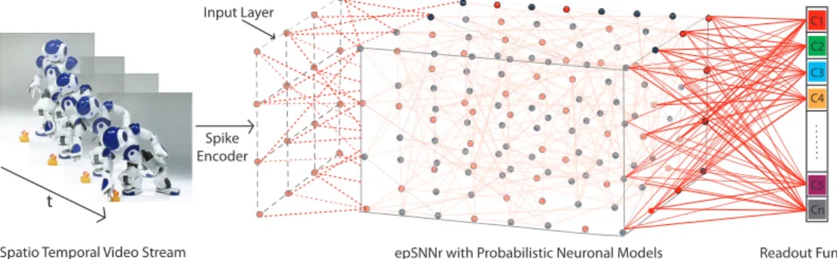
4.2 The proposed epSNNr Architecture . . . 66
4.3 Probabilistic neuronal models in the epSNNr as extensions of the LIF model . . . 68
4.4 epSNNr Pilot Study: Synthetic Video Dataset . . . 71
4.5 Design of the experiment . . . 72
4.6 epSNNr parameter settings . . . 75
4.7 Experimental results and discussions . . . 76
4.8 Summary . . . 78
5 Address Event Representation (AER): a method and its im-plementation 79 5.1 Artificial Silicon Retina - Neuromorphic Hardware utilizing AER . 81 5.2 Artificial Silicon Retina - Software Simulator utilizing AER . . . . 84
5.3 Summary . . . 90
6 Dynamic Evolving Spiking Neural Network (deSNN): a new generic method 91 6.1 Evolving Spiking Neural Networks (eSNN) . . . 92
6.2 The proposed Dynamic Evolving Spiking Neural Network (deSNN) 98 6.3 deSNN Examples . . . 104
6.4 Discussion . . . 109
6.5 Summary . . . 110
7 AER based Simple Motion Recognition with the deSNN method 111 7.1 Introduction . . . 112
7.2 Experimental Setting and Results for deSNN . . . 114
7.3 Summary . . . 118
8 A Novel epSNNr Architecture for Visual Data (epSNNA-v)120 8.1 A Novel Evolving Probabilistic Spiking Neural Network Architec-ture for spatio-temporal data (epSNNA-v) . . . 121
8.2 Data Acquisition Module . . . 123
8.3 Transformation Module . . . 123
8.4 Learning Module . . . 125
8.5 Summary . . . 126
9 Human Action Recognition with epSNNA-v 127 9.1 Case Study: AER based Human Action Recognition . . . 128
9.3 Experimental settings and results for deSNNr and learning deSNNr 134
9.4 Summary . . . 136
10 A Novel eSNN Architecture for Spectro-Temporal Data (epSNNA-s) 138 10.1 A Novel Evolving Spiking Neural Network Architecture for Spectro-Temporal Data (epSNNA-s) . . . 139
10.2 Data Acquisition Module . . . 139
10.3 Transformation Module . . . 145
10.4 Learning Module . . . 146
10.5 Summary . . . 147
11 Spectro-Temporal Pattern Recognition using the epSNNA-s148 11.1 Spectro-Temporal Dataset . . . 150
11.2 Case Study: Heart Sound Dataset . . . 154
11.3 Case Study: Isolated Spoken Words Dataset . . . 160
11.4 Summary . . . 165
12 Conclusion and future directions 167 12.1 Introduction . . . 167
12.2 Summary of achievements . . . 168
12.3 Future directions . . . 174
References . . . 179
A Appendix: Algorithms 196 A.1 KEDRI’s AER Software Simulator . . . 196
A.3 deSNN Algorithm . . . 198 A.4 Reservoir . . . 201
List of Figures
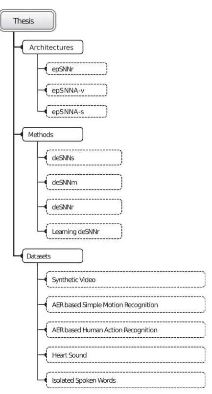
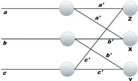
1.5.1 Architectures and methods developed in this study and datasets used for evaluating their performance. . . 8 2.3.1 Bain’s summation threshold network. It illustrates the way in
which the connections in a neural network can channel activation in different directions. The fiber a branches into two a′
, a′
; the fiber b into b′
, b′
; and cbranches into c′
, c′
. One of the branches a′
of a unites with one of the branches b′
of b, in a cell X; b′
and c′
unite in Y; a′
, c′
2.3.2 Hodgkin-Huxley type models represent the biophysical charac-teristic of cell membranes. The lipid bilayer is represented as a capacitance (Cm). Voltage-gated and leak ion channels are
represented by nonlinear (gn) and linear (gL) conductances,
re-spectively. The electrochemical gradients driving the flow of ions are represented by batteries (E), and ion pumps and exchangers are represented by current sources (Ip). Adapted from Hodgkin
and Huxley (1952c). . . 21 2.4.1 Schematics of Biological Neuron illustrating signal propagation
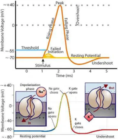
and synapsis. Taken from Wikipedia (2010) . . . 26 2.5.1 Action potential schematics: an ideal action potential shows its
various phases as the action potential passes a point on a cell membrane. Adapted from Wikipedia (2010). . . 31 2.5.2 The figure shows the probabilistic parameters used to extend the
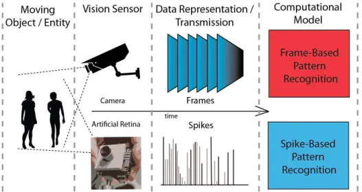
LIF model. This probabilistic neuron model was introduced by Kasabov (2010b). . . 41 2.6.1 This conceptual diagram illustrates the difference between the
Frame-based (top) and Spike-based (bottom) vision sensor, data representation and processing system. Depending on the com-putational model, the Frame-based method may involve compu-tationally intensive pre-processing steps such as feature selection and spike encoding, thereby rendering the Spike-based method faster and computationally less intensive. . . 46
2.6.2 These two plots show the idealized pixel encoding and reconstruc-tion of video data. The ON and OFF events represent significant changes in log I. It can be seen that changes greater than the threshold generate events, while changes that are smaller than the threshold are still represented internally in the differentiator. Adapted from Lichtsteiner and Delbr¨uck (2005). . . 47 4.2.1 A generic epSNNr architecture for spatio-temporal data modeling
and pattern recognition. . . 67 4.4.1 The figure illustrates the synthetic video dataset. There are four
classes corresponding to the 4 different directions of the object movement where each class consists of five samples. The arrows represent the direction in which the objects are moving. . . 71 4.5.1 The figure shows the raster plots and PSTH of 4 typical states for
the 4 classes produced by Step-wise Noisy Threshold (SNT). The top row shows the raster plot of the neural response of epSNNr with SNT probabilistic neurons recorded in 64 repetitions. The bottom row presents the corresponding smoothed PSTH for each raster plot. Each column corresponds to 4 different classes as indicated by the plot labels. . . 73 5.1.1 The figure shows the artificial silicon retina (DVS 128). This
neuromorphic hardware was used to acquire data for experiments in our study. . . 81 5.1.2 The figure shows the two different lighting conditions under
which the AER data was recorded for the Human Action Recog-nition Dataset using Artificial Silicon Retina (DVS128). . . 82
5.1.3 The figure shows the noise captured by the Artificial Silicon Retina when focused on fluorescent light source such as a tube light. The photo on the left shows the actual image and the plot on the right shows the AER snapshot. . . 83 5.1.4 The figure shows the raster plot, i.e. the spikes that represent
noise captured by the Artificial Silicon Retina when focused on fluorescent light source such as a tube light. The seven different spike colors represent noise from seven samples. The plot on the left is the raster plot for noise under fluorescent light conditions and figure on the right is the raster plot for noise under natural light conditions. . . 83 5.1.5 This bar graph compares the noise level from AER data acquired
under fluorescent (left) and natural (right) light conditions. . . . 84 5.2.1 (a) shows the disparity map of a video sample from KTH
dataset (Schuldt, Laptev, & Caputo, 2004). (b) shows the Ad-dress Event Representation (AER) generated by our simulator for Video Sample shown in (a). Here the red and blue color represent the On and Off events respectively. . . 85 5.2.2 These figure shows the idealized pixel encoding and
reconstruc-tion of video data. The ON and OFF events represent significant changes in log I. It can be seen that the changes are greater than the threshold generated events. Adapted from (Lichtsteiner & Delbr¨uck, 2005). . . 86
5.2.3 The figure shows the On and Off spike events for three human actions, namely a) Boxing, b) Hand Clapping and c) Jogging. It can be seen that the On and Off event map for each of the actions are quite similar especially for actions such as a) Boxing and b) Jogging. All the above three actions are performed by subject 1. At this stage we notice that the AER spike encoding for each of the actions are very much distinctive. . . 87 5.2.4 The figure shows that similar actions such as Walking, Running
and Jogging produce spike events that are visually alike. In this figure we have only shown ’On’ spike event map for 4 different subjects for easy comparison. It can be observed that different subjects performing the same action produce characteristically different spiking events. . . 88 5.2.5 The above figure shows the spiking events for four actions,
namely boxing, walking, running and hand clapping performed by the same subject. For each of the four activities the corre-sponding AER spike events, spikes from LSM using LIF neuron model and spikes from LSM using ST neuron model are pre-sented. The x-axis represents time in milliseconds for LSM and time in seconds for AER. The y-axis represents the number of neurons . . . 89 6.1.1 Integrate-and-fire neuron with RO learning . . . 95 6.1.2 eSNN for classification using population coding of inputs. Taken
6.2.1 An illustration of the STDP learning rule. Taken from (S. Song, Miller, Abbott, et al., 2000) . . . 102 6.2.2 An example of using SDSP neurons. Taken from (Brader, Senn,
& Fusi, 2007) . . . 102 6.3.1 A simple example to illustrate the main principle of the deSNN
learning algorithm. . . 105 6.3.2 This figure illustrates example 2 where two spatio-temporal
pat-terns are to be learned by two output neurons. . . 107 6.3.3 This figure shows the initial and final synaptic weights for
pat-terns 1 and 2 for the first four neurons. The difference in final weights for the two spatio-temporal pattern can be clearly seen. 107 7.2.1 Raster plots for the AER encoded samples from the Crash and
No crash classes. It can be seen that there is a similarity between the spike trains of Crash class, sample 1 (left figure) & No crash class, sample 2 (right figure). . . 115 7.2.2 The figure shows the spike raster plot, weights change and the
membrane potential (for neuron 0) for the eSNNs that utilizes rank order without the SDSP dynamics . . . 115 7.2.3 This figure shows the spike raster plot, weights change and the
membrane potential (mV) for the deSNNs. From the weights and the membrane potential graph (of neuron 0) it can be seen that due to the SDSP, the synaptic weights adjustments are faster compared to Fig. 7.2.2, for the sample from the same class . . . 117
8.1.1 A novel generic architecture is an evolving probabilistic spiking neural network architecture for spatio-temporal pattern recogni-tion (epSNNA-v). It consists of three mail modules. . . 122 9.1.1 This figure shows the raster plots of two samples, for each of the
three classes, where the samples in the first column were obtained under natural lighting conditions, and those in the second column were obtained under florescent lighting conditions. The higher level of noise present in the samples obtained under florescent lighting is apparent. . . 130 10.1.1 A generic spectro-temporal pattern recognition framework
(epSNNA-s). . . 140 10.2.1 This figure shows the anatomy of human inner ear. The anatomy
of the basilar membrane (BM) and its location in the cochlea is also depicted in this figure. The cochleagram’s function is based on the working of cochlea. Adapted from Wikipedia (2012). . . . 142 10.2.2 The above figure represents the cochleagram based spike
encod-ing method. From the above figure, it can be seen that we use the same number of LIF neurons as the number of gammatone filters in cochleagram. . . 145 11.1.1 This figure shows the waveform and spectrogram of heart
mur-mur sound sample. The region in the waveform graph that is highlighted in light green shows significant presence of noise es-pecially within the 2 - 2.5 seconds range. This noise can also be seen in the spectrogram. . . 151
11.1.2 This figure shows the cochleagram for the heart murmur sample whose waveform and spectrogram are shown in figure 11.1.1. This figure shows the difference in sound processing between standard cochleagram and spectrogram (from figure 11.1.1), where the cochleagram-processed sound has significantly less noise.152 11.1.3 This figure shows the waveform of normal heart sound sample.
It can be seen that the normal heart’s waveform is much cleaner than the heart murmur sound. However, there is noise present from external sources which can be seen at the end of the waveform.153 11.2.1 The above figure shows the cochleagram encoded spikes for a
heart murmur sample. This cochleagram encoded spikes are fed to the LSM reservoir having STDP learning. The plot below shows the raster plot for LSM with STDP learning. It can be seen that the spikes are highly synchronous. . . 159
List of Abbreviations
AER: Address Event Representation ANN: Artificial Neural Network BPDC: Backpropagation-Decorrelation
deSNN: Dynamic Evolving Spiking Neural Network
deSNNr: Dynamic Evolving Spiking Neural Network Reservoir DVS: Dynamic Vision Sensor
ECOS: Evolving Connectionist Systems
epSNN: Evolving Probabilistic Spiking Neural Network epSNNA-s: epSNNr Architecture for Spectro-Temporal Data epSNNA-v: epSNNr Architecture for Spatio-Temporal Data
epSNNr: Evolving Probabilistic Spiking Neural Network Reservoir ESN: Echo State Network
eSNN: Evolving Spiking Neural Network GRN: Gene Regulatory Network
LIF: Leaky Integrate-and-Fire Neuron LSM: Liquid State Machine
NR: Noisy Reset Neuron Model NT: Noisy Threshold Neuron Model ROSC: Rank Order Spike Coding SDSP: Spike-Driven Synaptic Plasticity SNN: Spiking Neural Network
SNT: Step-wise Noisy Threshold Neuron Model SOM: Self-Organizing Map
SSTD: Spatio- and Spectro-Temporal Data STDP: Spike-timing dependent plasticity STPR: Spatio-Temporal Pattern Recognition TSC: Temporal Spike Coding
Abstract
Video and audio information is spatio- or spectro- (sound/frequency) temporal in nature and processing of such complex Spatio/Spectro Temporal Data (SSTD) is a challenging task in the machine learning domain. SSTD contains both the spatial (space) and temporal (time) components and most often both these two components are highly correlated.
Due to the existence of high correlations between these two components, it is essential to process them together. However, many of the existing
computational methods either process spatial and temporal components separately, or processing them together then the significant correlation
information present in the SSTD is not considered. Comparatively, the brain is capable of performing such tasks in a fast and robust manner. Inspired by the innate cognitive functions of our brain, the proposed study investigates how various biological and cognitive aspects such as learning, evolution and neural information processing tasks can be applied to our computational model. We have shown that this enables efficient data acquisition, processing and learning of complex video and audio patterns thereby resulting in improved classification
performance.
This thesis proposes novel frameworks and classification methods employing a class of evolving spiking neural networks (eSNN) called dynamic evolving
spiking neural networks (deSNN) along with reservoir computing. In our study, we have shown that using the proposed frameworks results in (1) better
classification performance when compared to standalone spiking neural network classifiers such as eSNN, (2) better understanding of the data and the problem being solved, (3) faster SSTD processing due to the online one-pass spike-based computational approaches.
All the frameworks and methods proposed in this thesis have been evaluated on synthetic and real world problems. In order to evaluate the efficacy of the new methodology, initially a pilot experiment has been performed as a
benchmark test using a synthetic video dataset, followed by experiments on real world problems relating to motion and sound such as human action recognition and heart sound recognition.
“There are billions of neurons in our brains, but what are neurons? Just cells. The brain has no knowledge until connections are made between neurons. All that we know, all that we are, comes from the way our neurons are connected.”
Allen (2009)
1
Introduction
Existing statistical and artificial neural networks (ANN) machine learning approaches fail to model the complex spatio-temporal dynamics optimally. Since they either process spatial and temporal component separately the significant correlation information present in the Spatio and Spectro-Temporal Data (SSTD) is lost. Some of the existing methods that do consider both the space and the time component often input the spatio-temporal and
frame-by-frame basis. The historical information / event influences future events, hence they share a level of correlation with the future events occurring over time. Many of the traditional machine learning systems fail to consider the entirety of the SSTD pattern, therefore losing the significant spatio-temporal correlation information. This study takes the current spiking neural network based approach in machine learning to new conceptual and operational levels. We have proposed a spiking neural network (SNN) learning approach utilizing the spatio- and spectro-temporal architectures (epSNNA-v and epSNNA-s) that are expected to successfully achieve this holistic integration of spatio- and spectro-temporal events; they can also be further applied to solving real world problems. These architectures allow us to process continuous SSTD in a faster and computationally efficient manner.
1.1
Rationale and Significance of the Study
In spite of the recent research and development of SNN, there is a significant gap in finding the most effective approach and method for processing SSTD. This research aims at addressing this challenge with the development of a new SSTD modeling technique using evolving probabilistic Spiking Neural Networks (epSNN) for AudioVisual pattern recognition, including epSNN reservoir
systems (epSNNr).
Initial studies on reservoir systems such as Liquid State Machine (LSM) have shown promising results. Also, the evolving and stochastic nature of our system
will allow the model to adapt to new incoming data and learn incrementally. Moreover, the spikebased computation approach is expected to improve the processing time and accuracy considerably.
Video and audio information are spatio- or spectro- (sound/frequency) temporal in nature and processing such complex SSTD is a challenging task in the machine learning domain. Recent studies (Hamed, Kasabov, Shamsuddin, Widiputra, & Dhoble, 2011; Schliebs, Hamed, & Kasabov, 2011; Mohemmed, Schlibes, Matsuda, & Kasabov, 2012) have shown the SNNs capability of processing the SSTD simultaneously while retaining the significant correlation information between the space and time component. Therefore, we hypothesize that spiking neural network based methods and architectures will be capable of processing SSTD from real-world in a fast, one-pass, on-line and efficient
manner.
1.2
Definition and Motivation
The human brain studies date back many years. The recent scientific advances (such as electronics, cognitive and computer science) have made it possible to partially emulate the human brain and its innate cognitive ability. Learning is one such innate cognitive ability which has empowered the living animate entities and especially humans with intelligence. It is demonstrated by the ability to acquire new knowledge and skills that enable them to adapt and survive.
The exact working of the human brain is still only partially understood. It is assumed that the human brain’s ability to learn arises from the vast number of neurons and their interconnections. The number of connections for a neuron can range from 1000 to 200000 (Haykin, 1994). The latest study by Azevedo et al. (2009) show that the average human brain (weighing 1,508.91± 299.14 g,
age ≈ 50 years) has on average about 86.1 ± 8.1 billion (86.1 x 10¹¹) neurons.
The artificial neural networks are modeled after the most basic unit of the brain called neuron. Due to this there is certain similarity between artificial and biological neurons, and thus a biological counterpart for a component can always be found in an artificial neuron. Comparison between the biological and artificial neurons makes similarities between the two more evident.
Although, many existing traditional machine learning methods perform classification tasks much better than the artificial neural network, its ability is still not comparable to the any of the species biological neural network
especially the human brain. Since the ultimate goal of machine learning is to carry out cognitive tasks similar to the human brain, it takes its inspiration from it.
Motivated by the brain’s ability to learn autonomously by means of biological neural networks, we are looking to develop biologically inspired methods and architectures, that are designed to mimic some aspects of humans’ cognitive learning ability. This study aims not only to further new developments in
artificial spiking neural networks (SNN), but also to demonstrate the potential of SNN’s, for solving real world problems that involve the modeling of SSTD.
1.3
Research Objectives
Considering the fact that some novel, generic and specific spike-based data processing methods are required for SSTD modeling and pattern recognition, the study is divided into several parts as follows: development of novel SNN based classification methods, development of a novel spatio-temporal
architecture, development of a novel spectro-temporal architecture, and applications for visual and audio SSTD processing.
Both methods and architectures can be applied to the real world problems either independently or in combination by using spike-based computation approach. Combining the two architectures with the novel classification
methods results in hybrid algorithms (deSNNr and learning deSNNr), which are finally employed to work on real world dataset.
Based on the above discussion, we have arrived at the following research objectives:
• Develop some new classification methods for SSTD based on eSNN; • Develop a new generic eSNN method for SSTD based on reservoir
• Develop a generic method and a system for spatio-temporal pattern
recognition using Address Event Representation (AER). This will allow a model to directly utilize input spikes produced by an artificial silicon retina for preprocessing;
• Develop a software simulator for artificial silicon retina. This will allow
the usage of visual data that has not been obtained from the artificial silicon retina;
• Develop a generic method and a system for spectro-temporal pattern
recognition;
• Through comprehensive experimental analysis, evaluate the classification
performance of the architectures and methods in different combinations.
• Demonstrate the feasibility and applicability of the developed generic
architecture and methods by applying them to visual and audio SSTD from real world problems.
1.4
Specific Research Questions
Corresponding to the research objectives, the following specific research questions pertaining to this study have been formulated:
• How to improve/extend the existing eSNN method for application on
spatio- / spectro-temporal pattern recognition problems?
• Which spike information encoding scheme will be appropriate for SSTD
• Can the reservoir computing approach improve the classification
performance? Will the addition of stochastic neuron models further improve the reservoir performance? What is the optimal parameter setting for the neural networks? Can the reservoir states consisting of spikes be directly utilized by SNN methods for processing?
• Will the developed system be capable of processing the entire SSTD set?
How will the developed system perform with data having varying spike-times and temporal length (in milliseconds and minutes)?
• Will the system be capable of performing fast, one-pass, on-line learning?
1.5
Scientific Contribution
Figure 1.5.1 presents a visual summary of datasets, classification methods and generic architectures used and developed in the study. The items included under the architectures and methods branches are the main contributions of the study.
Architectures: This study proposes three new generic architectures for spatio-temporal and spectro-temporal pattern recognition (Figure 1.5.1),
namely epSNNr, epSNNA-v and epSNNA-s. Each architecture consists of many modules such as reservoir, STDP learning in reservoir, stochastic neuron
models, spike encoding module and learning algorithms. In the later chapters, the generic architectures will be explained in more details.
Methods: Four new spiking neural network based generic classifiers are proposed in this thesis. The proposed deSNNm and deSNNs are extensions of
Isolated Spoken Words Heart Sound
AERbased Human Action Recognition AERbased Simple Motion Recognition Synthetic Video Datasets Learning deSNNr deSNNr deSNNm deSNNs Methods epSNNr epSNNA-s epSNNA-v Architectures Thesis
Figure 1.5.1: Architectures and methods developed in this study and datasets used for evaluating their performance.
the eSNN algorithm (S. Wysoski, Benuskova, & Kasabov, 2008). The other two methods called deSNNr and learning deSNNr are hybrid algorithms obtained by combining the earlier proposed architecture and deSNNm/s algorithms.
Datasets: We have used five datasets to evaluate the classification performance of the proposed architectures and methods. It includes one
synthetic video dataset for benchmark testing and four real world datasets. The datasets have been described in details in their respective chapters.
1.6
Publications
The content put forth in this thesis was partially published in a number of international conference and journal articles:
• Dhoble, K., Nuntalid, N., Indivery, G., Kasabov, N. (2012) Online
Spatio-Temporal Pattern Recognition with Evolving Spiking Neural Networks utilising Address Event Representation, Rank Order, and Temporal Spike Learning, Proc. WCCI 2012: IEEE World Congress on Computational Intelligence, IEEE Press, (pp. 17).
• Kasabov, N.,Dhoble, K., Nuntalid, N., Indivery, G. (May, 2013)
Dynamic evolving spiking neural networks for on-line spatio- and
spectro-temporal pattern recognition. Neural Networks, Elsevier, Volume 41, (pp. 188-201).
• Kasabov, N.,Dhoble, K., Nuntalid, N., & Mohemmed, A.
pattern recognition: A preliminary study on moving object recognition.
ICONIP 2011 - In 18th International Conference on Neural Information Processing, Springer, Heidelberg. LNCS 7064, pp.230-239, Shanghai, China.
• Mohemmed, A., Matsuda, S., Kasabov, N., & Dhoble, K. (2011).
Optimization of Spiking Neural Networks with Dynamic Synapses for Spike Sequence Generation using Particle Swarm Optimization. IJCNN 2011 - In Proceedings of International Joint Conference on Neural Networks, (pp. 2969-2974), San Jose, California.
• Hamed, H. N. A., Kasabov, K., Shamsuddin, S. M., Widiputra, H., &
Dhoble, K.(2011). An Extended Evolving Spiking Neural Network Model for Spatio-Temporal Pattern Classification, IJCNN 2011 - In Proceedings of International Joint Conference on Neural Networks, (pp. 2653-2656), San Jose, California.
• Dhoble, K., Kasabov, N., Indivery, G. (2013) Dynamic evolving Spiking
Neural Networks for Spectro-temporal pattern recognition, IEEE
Transactions on Neural Networks and Learning Systems, IEEE Press, (in preparation).
1.7
Structure of the thesis
This thesis is organized into twelve chapters. A brief summary of the chapters is presented in this section.
Chapter 1 provides an introduction to the study and its objectives
Chapter 2 presents a literature review covering the theory of neural networks. This is followed by a discussion about the differences between traditional
artificial neural networks, artificial spiking neural networks (SNN) and biological neural networks. Various mechanisms of the biological neural networks have also been explained in details in order to show the biological plausibility of the artificial spiking neural network. The main concepts related to spiking neural networks such as neuronal models, spike encoding methods, working memories, learning mechanisms and their applications have been discussed in this chapter.
Chapter 3 reviews recurrent spiking neural network reservoirs structures. It also presents a summary on various reservoir computing approaches.
Chapter 4 proposes new generic architecture called epSNNr. The epSNNr is a Liquid State Machine (LSM) reservoir using various stochastic neural models. A pilot study is carried out using synthetic video dataset to test the feasibility and applicability of the architecture. The classification performance of epSNNr is carried out with various traditional classifiers. Also, we have compared the classification performance of epSNNr using the traditional Leaky Integrate and Fire (LIF) neural model with various stochastic neural models. This pilot study provides us with the feasibility test of using LSM on an entire spatio-temporal data for a pattern recognition task.
the artificial silicon retina. The workings and advantages of the AER approach for motion recognition are presented. In our spatio-temporal pattern case studies, we have utilized the data obtained from the artificial silicon retina. Therefore, we have discussed the attributes of the data obtained through this method. Also, developed as a part of this study, a software simulator of AER is presented.
Chapter 6 contains one of the main contributions of this thesis which is a novel dynamic evolving spiking neural network (deSNN) method. It is an extension of the evolving spiking neural network (eSNN) proposed by S. Wysoski,
Benuskova, and Kasabov (2008). This chapter introduces the eSNN method which is a part of evolving connectionist systems (ECOS) (Kasabov et al., 1998; Kasabov, 2002, 2003; Watts, 2009), followed by the characteristics and specifics of the two deSNN classifiers.
Chapter 7 presents how deSNN classifiers are applied on AER data obtained from the artificial silicon retina. This feasibility study provides us with a working proof on the ability of the deSNN method. Since the output of the AER based artificial silicon retina is in the form of spikes, we show that deSNN method is able to carry out direct spike-time computation instead of the
traditional frame-by-frame based computation. Also, a classification performance comparison is carried out between spiking neural network classifiers consisting of eSNN, deSNN and a feed-forward network with spike-driven synaptic plasticity learning rule (SDSP-SNN).
Chapter 8 presents a novel spiking neural network architecture for
spatio-temporal pattern recognition (epSNNA-v) along with two new methods namely deSNN reservoir (deSNNr) and learning deSNNr. All the earlier proposed methods, stochastic neuronal models, AER spike encoded data and the reservoir are incorporated into this generic architecture.
Chapter 9 evaluates the performance of the proposed epSNNA-v architecture for spatio-temporal data. Real world human action recognition data acquired from the AER silicon retina is used for performance comparison.
Chapter 10 proposes a new generic architecture for spectro-temporal pattern recognition (epSNNA-s). The proposed generic architecture epSNNA-s is different from epSNNA-v in terms of the spike information encoding scheme.
Chapter 11 evaluates the performance of the proposed epSNNA-s architecture two case studies, namely Heart Sound dataset and Isolated Spoken Words dataset.
Chapter 12 concludes the thesis by summarizing the achievements of the work and contains the overall conclusion. Neuromorphic hardware implementation and applications are also briefly discussed as future directions.
1.8
Summary
This chapter provides the background, motivation, research objectives and research questions addressed in this research.
More background information on the problem of SSTD modeling and pattern recognition can be found from the web page of EV FP7 Marie Curie funded project EvoSpike (http://ncs.ethz.ch/projects/evospike) led by Prof. Nikola Kasabov and Prof. Giacomo Indiveri, in which the candidate (myself) also took part.
The next chapter reviews the main aspects of spiking neural networks (SNN) which are used in this study to derived the generic SNN architectures and methods.
“In the study of brain functions we rely upon a biased, poorly understood, and frequently unpre-dictable organ in order to study the properties of another such organ; we have to use a brain to study a brain.”
Corning and Balaban (1968)
2
Why use Spiking Neural Networks for
SSTD?
In order to justify our methodology, it is necessary to become acquainted with various approaches to modeling Spatio / Spectro-Temporal Data (SSTD) and some SNN principles along with the expected benefits and possible inherent limitations. Here we have outlined the past and present research relevant to our study and have explained how our research addresses some of the issues in the
machine learning domain.
In the following subsection, we provide a brief introduction to the SSTD modeling techniques that have been researched and the inherent limitations they contain.
2.1
What is SSTD and why it is difficult to process it?
Video and audio information is spatio- or spectro- (sound/frequency) temporal in nature and processing of such complex Spatio-/Spectro-Temporal Data (SSTD) is a challenging task in the machine learning domain. SSTD contains both the spatial (space) and temporal (time) component and most often both these components are highly correlated.
Due to the existence of strong correlations between these two components, it is essential to process them together. However, many of the existing
computational methods either process spatial and temporal components separately or when processing them together the significant correlation information present in the SSTD is ignored. However, the brain is capable of performing such tasks in a fast and robust manner. Inspired by the innate cognitive functions of the brain, the proposed study investigates how various biological and cognitive aspects such as learning, evolution and neural information processing can be applied to our computational model.
2.2
SSTD Processing Approaches
Many of the traditional machine learning systems fail to consider the entirety of the SSTD pattern, therefore losing the significant information about the
spatio-temporal correlation. This study takes the innovative work in machine learning done at KEDRI to new conceptual and operational levels. We have proposed a novel machine learning approach utilizing the epSNNr architecture that is expected to successfully achieve this holistic integration of
spatio-temporal events. The new approach would allow us to process continuous SSTD in a faster and computationally efficient manner.
Hidden Markov Models (HMM) is one of the popular statistical approaches that is widely used for processing temporal information (Rabiner, 1989). It is often used either with traditional neural networks (Trentin & Gori, 2001) or on its own (Waibel et al., 1989; Poppe, 2010). However, it has an inherent
limitation when defining the HMM for more than a single independent variable. This means that they can only be defined for a process that is a function of a single variable, such as time or one-dimensional position (Trentin & Gori, 2001; Turaga et al., 2008), rendering them incapable of optimally learning from SSTD patterns which are two-dimensional in nature. Also, there are other emerging approaches such as deep machine learning which involves the combination of Deep Belief Networks (DBNs - Generative Model) and Convolutional Neural Networks (CNNs - Discriminative Model) (Arel, Rose, & Karnowski, 2010). The proposed DBNs model nevertheless carries out learning in a frame by frame manner, rather than learning the entire SSTD patterns. On the other hand,
Gerstner and Kistler (2002b) state that the brain-inspired SNN has the ability to learn spatio-temporal patterns by using trains of spikes (which are
spatio-temporal events). Furthermore, the 3D topology of the spiking neural network reservoir allows us to capture the whole SSTD patterns at any given time points. The neurons in this reservoir system transmit spikes via synapses that are dynamic in nature, collectively forming a SSTD memory (Maass & Zador, 1999; Maass & Markram, 2002). Often, learning rules such as
Spike-Time-Dependent-Plasticity (STDP) (Legenstein, Naeger, & Maass, 2005) are commonly utilized in SNN models.
Recently, several SNN models and their applications have been developed by numerous research groups (Verstraeten et al., 2007; Buonomano & Maass, 2009; Maass et al., 2002; Brader et al., 2007; Bohte & Kok, 2005; Natschlager & Maass, 2002) as well as by our research group at KEDRI (Kasabov, 2007; S. Wysoski et al., 2010; Soltic & Kasabov, 2010a; Kasabov, 2010a; Schliebs, Kasabov, & Defoin-Platel, 2010; Soltic & Kasabov, 2010b; S. Wysoski et al., 2008; Kasabov, 2010b). However, they process the SSTD as a sequence of static feature vectors extracted from segments of data, without utilizing the SNN’s capability of learning whole SST patterns.
2.3
A brief History of Neural Networks
The study of human anatomy, especially brain studies date back thousands of years. The recent advances in science (such as electronics, cognitive and
innate cognitive ability. This section introduces the general underlying
principles of neural networks as well as the strengths and weakness of different types of neural network and how they relate to each other. Some of the most significant neural network designs are presented in details below.
In late 18 century, based on the neuroanatomical findings led by the neurobiologists such as Gerlach (1858), Nissl (1858), and Waldeyerin (1863) (Swanson, 2000; Nissl, 1894), Alexander Bain presented the first neural network in his 1873 book entitled ”Mind and Body. The Theories and Their Relation” (Wilkes & Wade, 1997).
Figure 2.3.1: Bain’s summation threshold network. It illustrates the way in which the connections in a neural network can channel activation in different directions. The fiber
abranches into two a′
,a′
; the fiberb intob′
,b′
; andc branches intoc′
,c′
. One of the
branches a′
of aunites with one of the branchesb′
ofb, in a cell X;b′
andc′
unite in Y;
a′
,c′
in Z. Adapted from Wilkes and Wade (1997).
In 1943, Warren McCulloch and Walter Pitts designed and built a primitive artificial neural network using simple electric circuits that formed the basis for modern era of neural network research (McCulloch & Pitts, 1943; Haykin, 1994).
There was significant development after the publication of ’The Organization of Behavior: A Neuropsychological Theory’ by Hebb (1949). It introduced theoretical concepts such as cell assembly, phase sequence, and Hebb synapse that set forth his hebbian learning rule. The major point brought forward was the strengthening of neural pathways after each use. This rule is especially applicable for the more bio-plausible spiking neural networks. Hebb (1949) findings further reinforced McCulloch-Pitts’s theory on neurons and their functions (Haykin, 1994).
With the emergence of computers in the 1950s, the neural models were ported from hardware to the digital realm. Alan Lloyd Hodgkin and Andrew Huxley described a scientific model of a spiking neuron in 1952 (Hodgkin & Huxley, 1952a, 1952b, 1952c). They explained the ionic mechanisms underlying the initiation and propagation of action potentials in the squid giant axon. Hodgkin-Huxley model is widely regarded as one of the great achievements of 20th-century biophysics that describes how action potentials in neurons are initiated and propagated (Hodgkin & Huxley, 1952a, 1952b, 1952c).
In 1954 Marvin Minsky carried out research on neural networks (Minsky, 1954) that was presented in his doctoral dissertation titled ”Theory of
Neural-Analog Reinforcement Systems and its Application to the Brain-Model Problem” (Harmon, 1962). In 1957, John von Neumann anticipated that computer design based on brain had great prospects and could be implemented by using telegraph relays or vacuum tubes to emulate simple neuron functions.
Figure 2.3.2: Hodgkin-Huxley type models represent the biophysical characteristic of
cell membranes. The lipid bilayer is represented as a capacitance (Cm). Voltage-gated
and leak ion channels are represented by nonlinear (gn) and linear (gL) conductances,
respectively. The electrochemical gradients driving the flow of ions are represented by
batteries (E), and ion pumps and exchangers are represented by current sources (Ip).
Adapted from Hodgkin and Huxley (1952c).
This idea led to the invention of the von Neumann machine (Boahen, 2007). Later, Minsky went on to publish the first paper on artificial intelligence entitled ”Steps Towards Artificial Intelligence” (Minsky, 1961).
In 1958, based on the idea of McCulloch-Pitt’s theory and research done on the fly’s eye, a neurobiologist named Frank Rosenblatt worked on the idea of perceptron. He built the first artificial neural network realized in hardware (Masters, 1993).
In 1960, Bernard Wildrow and Marcian Hoff developed the Adaptive Linear Neuron or later known as Adaptive Linear Element (ADALINE) and Multiple
Adaptive Linear Neuron (MADELINE) models which were the first neural networks applied to real problems. ADALINE is a convergent type single layer neural network based on the McCulloch-Pitts neuron consisting of a weight, a bias and a summation function. It’s used for prediction involving binary
patterns as its input and one output. Similarly, for problems requiring multiple outputs, multiple sets of ADALINEs are used in parallel and this model is known as MADELINE. These models introduced the then novel least mean square (LMS) error training algorithm, also called the Widrow-Hoff Delta Rule (Widrow & Lehr, 1990). ADALINE perceptrons learning procedure is attractor driven (positive reinforcement) in which a convergent subcircuit output value is specified as the goal for each pattern. Therefore, it is necessary for the
subcircuit to learn the proper weight values to produce that goal value for any input patterns. Later perceptrons (negative reinforcement type) used
misclassification errors instead of using a defined goal for each subcircuit (Widrow & Hoff, 1988; Widrow & Lehr, 1990; Widrow, 2005). In the standard McCulloch-Pitts based perceptron, the weighted sum of the inputs is passed to the activation (transfer) function and its output is used for adjusting weights. Whereas in ADALINE, based on weighted sum of the inputs, the weights drawn from subcircuits are adjusted in the learning phase.
Kohonen introduced self-organizing maps (SOMs) in the 1970s, also
commonly known as Kohonen networks (Kohonen, 1989; Kohonen & Honkela, 2007). SOM is an artificial neural network used for visualization and analysis of high-dimensional data in an unsupervised setting. It uses a neighborhood function to preserve the topological properties of the high dimensional input
space when projecting it into a low dimensional discretized space called Kohonen map (Kohonen, 1989).
Hopfield (1982) introduced a new form of recurrent artificial neural network as content-addressable memory systems (associative memories) with binary threshold units. This form of ANN is now also known as Hopfield network. The Hopfield networks convergence properties could be analyzed due to the
introduction of the energy function. A Hopfield network can be used as an associative memory through Hebbian learning (Hopfield, 1988; Sulehria & Zhang, 2007; Haykin, 1994).
Powell (1987) invented the Radial-Basis Function (RBF) network in 1985. The idea for RBF originates from older pattern recognition techniques (Tou & Gonzalez, 1974) such as potential function, clustering, functional
approximation, mixture models and spline interpolation. The RBF employs a clustering algorithm to find the most prominent clusters in the input
hyperspace of multivariate data. It then linearly combines hyperspheres around these clusters to determine the classifications of specific input patterns based on previously classified training patterns (Powell, 1987). RBF networks are able to model complex mappings due to their nonlinear approximation properties, whereas perceptrons can only model by means of multiple intermediary layers (Haykin, 1994).
First introduced by Bryson and Ho (1975), the Backpropogation neural networks gained recognition through the work of David E. Rumelhart, Geoffrey
E. Hinton and Ronald J. Williams in 1986 (Russell & Norvig, 1995; Rumelhart, Hinton, & Williams, 1986). They extended the Widrow and Hoff’s delta rule to networks with multiple hidden layers by means of generalized delta rule. This model was based on the perceptron and came to be known as the Back
Propagation Network. Back Propagation requires differentiable activation (transfer) function. It is one of the most widely used artificial neural network model.
The underlying mechanisms of the Back Propagation paradigm, which solved the problem of training hidden neuron layers, was actually discovered earlier by Paul Werbos in 1974 (Werbos, 1974, 1994), and Parker and LeCun (Parker, 1985; LeCun, 1985, 1986) in 1985, but it was Rumelhart (Rumelhart, Hinton, & Williams, 1986) who made it universally known.
The Boltzmann machine is a type of stochastic recurrent neural network introduced in 1986 by Geoffrey Hinton and Terry Sejnowski (Hinton &
Sejnowski, 1986). The Boltzmann machine is derived from Hopfield network but with sophisticated elaborations like the inclusion of annealing and stochastic processes used for tasks such as pattern completion; therefore it is used for solving pattern classification problems with noisy, incomplete data (Hinton & Sejnowski, 1983b, 1983a, 1986). Similar to Hopfield network, the Boltzmann machine has an energy function defined for the network but it is different from the Hopfield network as it is stochastic in nature (Ackley, Hinton, & Sejnowski, 1987).
feed-forward network modified by one or more feedback connections (Elman, 1991). The ”Elman net” functionality produces a pattern-holding reservoir over a certain period of time, therefore allowing detection of temporal patterns in time series.
More recently spiking neural networks (SNN) (Gerstner & Kistler, 2002a; Izhikevich, 2003) have been developed. SNNs belong to the third generation of neural networks. Their mechanism is more realistic in terms of their spiking processes resembling the biological neurons (Maass & Bishop, 1999). In the following section we explain why SNNs are advantageous over traditional neural networks.
2.4
Spiking Neural Networks
The exact workings of the human brain still remain a mystery to the scientific community. It is assumed that the human brain’s capability arises from the vast number of neurons and their interconnections. The number of connections for a neuron can range from 1000 to 200000 (Haykin, 1994). The latest study by Azevedo et al. (2009) shows that the average human brain (weighing 1,508.91 ±
299.14 g, age≈ 50 years) has on average about 86.1 ± 8.1 billion (86.1 x 10¹¹)
NeuN-positive cells (“neurons”).
We do not understand the exact workings of the brain yet. In fact,
understanding the functioning of a single neuron and its chemical synapses in itself proves to be much more complex than previously assumed.
Figure 2.4.1: Schematics of Biological Neuron illustrating signal propagation and synap-sis. Taken from Wikipedia (2010)
The artificial neural networks are modelled after the most basic components of the brain, which is the neurons. There is a strong similarity between artificial and biological neurons, and thus a biological counterpart for a component can always be found in an artificial neuron. When comparing the biological and artificial neurons, similarities between the two become more evident.
SNNs are made up of artificial neurons that use trains of spikes to represent and process pulse-coded information (Maass & Bishop, 1999). The biologically realistic information processing capability of spiking neural networks will allow the development novel neural models that enhances the ability to solve various problems. Gerstner and Kistler (2002a) stated that, in order to avoid any prior
assumptions on neural computation, the processing and exchange of information between neurons should be carried out at the level of spikes. This resulted in the emergence of spiking neural networks as the new generation of neural network models that are imperative to the computational functionality.
In biological neural networks, neurons are connected at synapses and electrical signals (spikes) pass information from one neuron to another. SNNs are biologically plausible and offer some means for representing time, frequency, phase and other features of the information being processed. This allows
incorporating spatio-temporal information in communication and computation, similarly to real neurons. There are many models of biological spiking neurons such as Hodgkin-Huxley’s model (Hodgkin & Huxley, 1952c), Spike Response Models (SRM) (Gerstner, 1995; Kistler, Gerstner, & van Hemmen, 1997; Gerstner & Kistler, 2002a), Integrate-and-Fire Models (Maass & Bishop, 1999; Gerstner & Kistler, 2002a), Izhikevich models (Izhikevich, 2004, 2006, 2007; Izhikevich & Edelman, 2008). Although numerous models of SNNs and their applications have been developed, they have not been successfully used for solving large scale, complex AI problems of classification, temporal and string sequence pattern recognition and associative memory (Kasabov, 2010b). According to Kasabov (2010b), since “the spiking processes in biological neurons are stochastic by nature it would be appropriate to look for new inspirations to enhance the current SNN models with probabilistic parameters” (Schliebs, Defoin-Platel, & Kasabov, 2009; Kasabov, 2009).
2.4.1 Spiking Neural Networks Versus Traditional Neural Net-works
Although SNNs can perform all the afore mentioned tasks of traditional neural networks, they have some additional capabilities in a range of domains such as;
1. Spatio-temporal domain (e.g. time series).
2. Complex domains requiring massive scale networks with several thousand neurons (e.g. VLSI).
3. Domains requiring biologically derived models (biological fidelity). Maass and Bishop (1999) state that compared to traditional ANNs, SNN requires fewer neurons to accomplish the same task (Maass & Bishop, 1999; Gerstner & Kistler, 2002a), it is more biologically plausible (Maass & Bishop, 1999) and has the capability of approximating any function. Moreover, since SNN uses spikes instead of analog values to communicate between neurons, they can be multiplexed (as binary codes) thereby requiring less time and space to compute.
SNNs are made up of artificial neurons that use trains of spikes to represent and process pulse coded information (Maass & Bishop, 1999). SNN use trains of spikes for internal information representation (Huguenard, 2000).
2.5
Neuronal Models
• neuronal models;
• encoding information into spikes; • learning algorithms;
• network structure and connectivity.
The counterpart or the abstraction of the biological neuron can always be found in the spiking neuron models. In order to understand why and how the SNN neuron models work, we have first provided a brief explanation of the workings of a biological neuron followed by the artificial neuron models.
2.5.1 Biological Neurons
The basic characteristics and parts of the neurons are identical to other cells; however, they are specialized cells that have the ability to gather and transmit electrochemical signals (i.e. communicate/pass messages to each other) over a particular distance. As illustrated in figure 2.4.1, a neuron has three basic parts:
Cell body: This part consists of cell components such as nucleus also sometimes referred to as the ”control center” (which contains genetic material), endoplasmic reticulum and ribosomes (for building proteins from amino acids.) and mitochondria (generates adenosine triphosphate (ATP), used as source of chemical energy).
Axons: These are long nerve fibers that carry electrochemical impulses (action potentials) away from the cell body or soma. Within the brain,
Dendrites: These nerve endings are branchlike projections of the cell that conduct the action potentials received from other neural cells to its cell body, or soma. Depending on the type of neuron, dendrites can exist on one or both ends of the cell.
2.5.2 Action potential
An action potential (nerve impulse) results from a brief change of membrane potential across an excitable membrane in a neuron that is produced due to the voltage-gated ion channels activity in the membrane (Purves et al., 2008). In order to understand how the initiation and transmission of nerve impulses take place in neurons, we need to understand the neurons structure and mechanism in details. The neurons cell membrane is made up of phospholipids. It is arranged in two-layer lipid sandwich with the electrically charged polar heads exposed to water and the polar tails sticking near each other, barricading the cell from the outside water-soluble or charged particles (such as ions). How exactly the charged particles get into the cells is explained in the next section.
Ion Channels
Ions are charged atoms (or water soluble molecules) that are able to move through channels that are present across the cell membranes (phospholipids) bilayer. Sodium, potassium, calcium and chloride ions have their own specific permeable channels in the cell membrane allowing the cell to maintain
Figure 2.5.1: Action potential schematics: an ideal action potential shows its vari-ous phases as the action potential passes a point on a cell membrane. Adapted from Wikipedia (2010).
of the cell membrane allows the maintenance of outside concentration of sodium to be 10 times higher than inside and inside potassium concentration to be approximately 20 times higher than cells outside. This creates a negative electrical charge (of about∼ 70 mV to ∼ 1 mV) inside the cell. The cell
membrane is semi-permeable, i.e. leaky, to the tiny positively charged sodium and potassium ions in the cells outside. This difference in charge between the cells inside and outside creates an affinity. The selective ion pumps spanning across the cell membrane uses ATP as energy for exchange of the sodium and
potassium ions across the cell membrane generating a tiny electrical current (as seen in Figure 2.5.1).
Nerve Signals
The action potential (i.e. nerve signal) is generated from the sodium and
potassium ions coordinated movement across the cell membrane. The details on how the action potential initiates is discussed below.
Action Potential Initiation:
As mentioned previously, the inside of a cell is negatively charged and has a resting membrane potential of approximately -70 to -80 mV. This chemical or electrical imbalance between the inside and outside cell fluid opens up some of the sodium ion channels in the cell membrane. The transfer of the positively charged sodium (+Na) ions into the cell results in depolarization (reduced negative charge inside the cell). When the depolarization reaches a certain threshold value, it opens more sodium ion channels. Consequently this triggers an action potential due to more inflow of sodium ions in the nerve cell. The high concentration of +Na ions (inside the nerve cell) reverses the local membrane potential. At this point as seen in Figure 2.5.1, the electrical potential inside the cell goes to about ∼ +40 mV. At this electrical potential,
the sodium ion channel closes resulting in sodium inactivation (inflow of sodium ion stops) and simultaneously triggers the opening of the potassium ion
toward the resting membrane potential and causes the shutdown of potassium ion channels. Although, the membrane potential overshoots the resting
potential, the ion balance is quickly restored by the sodium-potassium pump bringing the membrane potential to its resting level. This ion flux triggers an action potential (Hodgkin & Huxley, 1952c).
Action Potential Propagation
After the action potential is passed on to the next area of the cell membrane, the previous area enters into a refractory period (depolarizes again) preventing the backward movement of the action potential. Thus the action potential is conducted only in one direction at the speed of 10 to 100 meters per second through the axon depending on the type of neuron (Hodgkin & Huxley, 1952a, 1952b, 1952c). Since the size of action potential remains the same, it is assumed that the information is encoded by the frequency (pulse or rate code is still debatable) of action potentials (Maass & Bishop, 1999).
Synaptic Transmission
Synapsis is the gap between neurons where the communication occurs. Synaptic transmission is also known as neurotransmission that occurs due to the
propagation of action potential within the synapses through neurotransmitters. The neuron that sends the action potential is known as presynaptic neuron and the receiving neuron cell is called the postsynaptic neuron. There are several types of neurotransmitters such as glutamate, serotonin, acetylcholine,
norepinephrine, dopamine, gamma-amino butyric acid (GABA) etc. Also, a nerve cell may have synapses on it from excitatory presynaptic neurons and from inhibitory presynaptic neurons. In addition to neurotransmitters, there are neuropeptides that modulate the effects of groups of neurotransmitters and single neurotransmitters, over varying time scales (from milliseconds to days). Some of the neuropeptides are released from axonal terminals directly into the synaptic void, while others are released from hormone glands. This leads to a collective management of the control mechanisms that direct the action of intracellular ion flux.
As to how the synaptic transmission process takes place, neurotransmitter serotonin will be used as an example. The presynaptic cell makes serotonin (5-hydroxytryptamine, 5-HT) from the amino acid tryptophan and stores it in vesicles in its end terminals. When an action potential (called the presynaptic spike) passes down the presynaptic cell into its axonal terminals, the vesicles containing serotonin gets stimulated (by the action potential) to fuse with the cell membrane and releases the neurotransmitter into the synaptic cleft. The released serotonin traverses across the cleft and binds with receptors (ion
channels) on the membrane of the postsynaptic cell and causes depolarization in the postsynaptic cell. This is caused due to the influx of positive Na ions from the extracellular fluid, which thereby charges the intracellular fluid of the dendrite. As explained previously, when depolarizations reach a threshold level, a new action potential will be propagated in that cell. However, some
neurotransmitters hyperpolarizes the postsynaptic cell (more negatively
molecules in the synaptic cleft are then destroyed by enzymes such as
monoamine oxidase (MAO) and catechol-o-methyl transferase (COMT). Also some of the neurotransmitters are reabsorbed by the presynaptic cell
(reuptake), where MAO and COMT destroy the absorbed serotonin molecules. This prepares the synapse to receive another action potential. The soma, however, remains temporarily charged for a longer period than the dendrites, allowing it to work like an accumulation buffer (leaky reservoir) for new voltage promulgations from the dendrites (Hodgkin & Huxley, 1952c, 1952b, 1952a; Arbib, 2003; Amari & Kasabov, 1998; Purves et al., 2008).
2.5.3 Artificial Spiking Neuron Models:
Many of the traditional ANN’s neural models consisted of synaptic weights and activation / transfer function. The artificial neuron abstraction could be simply expressed in mathematical form as
yj =φ(
X
i
wijxi) (2.1)
where yj and xi are the neuronal output and input signals respectively, φ is the
activation function andwij represents the synaptic connection weight between
neurons i and j. Biological neurons, however, are described by ion currents that are transmitted through the cell membrane when neurotransmitters activate the ion channels in the cell. In order to simulate a biologically realistic neuron, many models have been proposed. The next section provides a short description on some of these neuron models.
Hodgkin-Huxley Model:
Based on the experiments on the giant axon of the squid, Hodgkin and Huxley found three different ion channels: sodium, potassium and a CI−
ions leak current (Hodgkin & Huxley, 1952b, 1952a, 1952c). The flow of ions through the cell membrane is controlled by voltage-dependent ion channels as explained previously. In mathematical terms, this model can be described as an electric circuit (see Fig.2.3.2) having a capacitance (C), batteries (E), and current sources (I). Thus, as seen in Fig.2.3.2, the current applied over time (I(t)), may be distributed as a capacitive current (IC) which charges the capacitor (C), and
the current (Ik) of each ion channel is:
I(t) =IC(t) +
X
k
Ik(t) (2.2)
where the P
k represents the sum of all ion channels. The capacitor (C) can
be defined as C =QIu, where Q and u are the charge and voltage across the capacitor. Therefore, charging capacitive current can be represented as
IC =C
du
dt (2.3)
Hence, according to Eq.2.2 and Eq.2.3:
Cdu dt =−
X
k
Ik(t) +I(t) (2.4)
channel model as:
X
k
Ik(t) =gN am3h(u−EN a) +gKn4h(u−EK) +gL(u−EL) (2.5)
where EN a, EK and EL are reversal potentials obtained from empirical
experiments. The gating variablesm, n and h evolve according to the differential equations
x=αx(u)(1−x)−βx(u)x (2.6)
where x represents m, n orh and αx, βx denote exponential function that can
be adjusted in order to simulate a specific neuron. It can be seen that the Hodgkin-Huxley model can reproduce electrophysiological measurements very accurately. However, due to the model’s complexity, it is computationally expensive, making it inappropriate for large networks of spiking neurons.
Leaky Integrate and Fire Model (LIF)
A LIF neuron is a simplified Hodgkin-Huxley model where all the ion channels are represented with a single current (Stein, 1967). Therefore, according to Eq.2.3 and IR =u/R (Ohm’s law) we get
I(t) = u(t) R +C
u
dt (2.7)
standard form
τm
du
dt =−u(t) +RI(t) (2.8)
where, uis the membrane potential, I(t) represents input current, τm is
membrane time constant and R represents (soma membrane) resistance. Apart from the stimulation by the external current I(t) =Iext(t) over time, in a
network the neurons can also be stimulated by presynaptic neuronj. The synaptic input of neuron i is the weighted sum over all the current generated by the presynaptic neurons and can be represented as :
Ii(t) = X j wij X f α(t−t(jf)) (2.9)
where, weight wij reflects the strength of the synapsis from neuron j to
neuron i,t(jf) represents the firing time of neuron j, while α represents the time
course of the postsynaptic current. The simplicity of the LIF model makes it suitable for use in large scale networks allowing efficient simulation.
Spike Response Model (SRM)
In Spike Response Model (SRM) (Lapicque, 1907; Hill, 1936; Brillinger, 1992; Gerstner, 1995; Keat, Reinagel, Reid, & Meister, 2001; Jolivet, Lewis, &
Gerstner, 2004), the state of the neuron i is defined by a single parameter ui(t)
(membrane potential). The LIF model can be considered as a special case of the general SRM that defines the spike dynamics. The ui continues to be at
threshold ϑ, the neuron fires and the membrane potential resets to its resting potential. Assuming that the neuron ihas fired its last spike at time ˆti, then
the evolution ofui after firing can be expressed as
ui(t) =η(t−ˆti)+ X j wij X f εij(t−ˆti, t−ˆt (f) j )+ Z ∞ 0 κ(t−ˆti, s)Iext(t−s)ds (2.10)
where the spike time of presynaptic neuron j is denoted by t(jf),η is a
function that describes the form of action potential and after potential, ε denotes the time course of the postsynaptic potential and wij represents
synaptic efficacy. The linear response of the membrane for external input current Iext is represented by kernal function κ. Compared to the LIF model,
the membrane threshold of SRM is not fixed but may depend on t−ˆti, hence
ϑ −→ϑ(t−ˆti) (2.11)
The SRM is ideal for simulating large number of neurons in a network due to its simplicity. Also, compared to LIF neuron, SRM allows to cover
refractoriness. The refractoriness is important because it allows forward propagation of emitted spike. This refractory period is due to the delay in closing of voltage-gated potassium channels that opened in response to depolarization. This delay causes extra potassium conductance and results in hyper polarization.
Fast Integrate and Fire Model
The system is based on SpikeNet introduced in (Delorme, Perrinet, & Thorpe, 2001; Delorme & Thorpe, 2003; S. G. Wysoski & Benuskova, 2006; S. Wysoski et al., 2008). The postsynaptic potential dynamics for neuron i can be
expressed as
ui(t) =
X
j
modorder(j)wij (2.12)
where order(j) determines the firing rank of neuronj, wij denotes synaptic
efficacy and mod∈[0,1]. The membrane potential ui fires on reaching threshold
ϑ and resets to resting potential after which the neuron is disabled. This neuron model is often used in image and speech recognition tasks due to its low <