Effects of ramped wall temperature and concentration on viscoelastic Jeffrey’s fluid flows from a vertical permeable cone

Effects of ramped wall temperature and 

concentration on viscoelastic Jeffrey’s 

fluid flows from a vertical permeable cone

Gaffar, SA, Prasad, VR, Beg, OA, Khan, MH and Venkatadri, K

http://dx.doi.org/10.1007/s40430­018­1354­7

Title Effects of ramped wall temperature and concentration on viscoelastic  Jeffrey’s fluid flows from a vertical permeable cone Authors Gaffar, SA, Prasad, VR, Beg, OA, Khan, MH and Venkatadri, K Type Article URL This version is available at: http://usir.salford.ac.uk/id/eprint/48158/ Published Date 2018 USIR is a digital collection of the research output of the University of Salford. Where copyright  permits, full text material held in the repository is made freely available online and can be read,  downloaded and copied for non­commercial private study or research purposes. Please check the  manuscript for any further copyright restrictions. For more information, including our policy and submission procedure, please contact the Repository Team at: [email protected].

JOURNAL OF THE BRAZILIAN SOCIETY OF MECHANICAL SCIENCES AND ENGINEERING PUBLISHER: SPRINGER

IMPACT FACTOR: 1.627

ISSN: 1678-5878 (PRINT VERSION); ISSN: 1806-3691 (ELECTRONIC VERSION) Accepted August 12th 2018

EFFECTS OF RAMPED WALL TEMPERATURE AND CONCENTRATION ON VISCOELASTIC JEFFREY’S FLUID FLOWS FROM A VERTICAL PERMEABLE CONE

S. Abdul Gaffar1*_{, V. Ramachandra Prasad}2_{, O. Anwar Bég}3_{, Md. Hidayathullah Khan}4_{, K. Venkatadri}5 1_{Department of Mathematics, Salalah College of Technology, Salalah, Oman}

2_{Department of Mathematics, School of Advanced Science, VIT University, Vellore, India}

3 _{Fluid Mechanics, Aeronautical and Mechanical Engineering Department, University of Salford, Manchester, M54WT, UK} 4_{Department of Mathematics, Sri Vishveshwaraiah Institute of Science and Technology, Madanapalle - 517325, India}

5_{Department of Mathematics, Vemu Institute of Technology, Kothakota, India}

ABSTRACT

In thermo-fluid dynamics, free convection flows external to different geometries such as cylinders, ellipses, spheres, curved walls, wavy plates, cones etc. play major role in various industrial and process engineering systems. The thermal buoyancy force associated with natural convection flows can exert a critical role in determining skin friction and heat transfer rates at the boundary. In thermal engineering, natural convection flows from cones has gained exceptional interest. A theoretical analysis is developed to investigate the nonlinear, steady-state, laminar, non-isothermal convection boundary layer flows of viscoelastic fluid from a vertical permeable cone with a power-law variation in both temperature and concentration. The Jeffery’s viscoelastic model simulates the non-Newtonian characteristics of polymers, which constitutes the novelty of the present work. The transformed conservation equations for linear momentum, energy and concentration are solved numerically under physically viable boundary conditions using the finite-differences Keller-Box scheme. The impact of Deborah number (De), ratio of relaxation to retardation time (), surface suction/injection parameter (fw), power-law exponent (n), buoyancy ratio parameter (N)

and dimensionless tangential coordinate () on velocity, surface temperature, concentration, local skin friction, heat transfer rate and mass transfer rate in the boundary layer regime are presented graphically. It is observed that increasing values of De reduces velocity whereas the temperature and concentration are increased slightly. Increasing  enhance velocity however reduces temperature and concentration slightly. The heat and mass transfer rate are found to decrease with increasing De and increase with increasing values of . The skin friction is found to decrease with a rise in De whereas it is elevated with increasing values of . Increasing values of fw and n, decelerates the flow and also cools the boundary layer i.e. reduces

temperature and also concentration. The study is relevant to chemical engineering systems, solvent and polymeric processes.

KEYWORDS:Viscoelastic Jeffrey’s fluid; implicit finite-differences method; Deborah number; relaxation time; retardation time; power-law index; suction/injection.

INTRODUCTION

In many fluids the flow properties are difficult to explain by a single constitutive equation like Newtonian model. Geological materials and polymer solutions used in different industries and engineering processes are such fluids which cannot be explained by Newtonian model. The materials that cannot be explained using Newtonian model are called Non-Newtonian fluid models. In past few decades, due to the applications in industries, engineering and technology, non-Newtonian fluid flows has gained interest in researchers. In such fluids the shear stress and strain rate relation is non-linear. The non-Newtonian fluid models are complicated and relate the shear stresses to the velocity field [1]. Different non-Newtonian fluid models have been discussed by different researchers that include oblique micropolar flows [2], Walter’s-B fluids [3], Jeffrey’s flows [4], Williamson fluid [5], nanofluid [6], Maxwell flows [7], Eyring-Powell flows [8], Tangent Hyperbolic flows [9], Oldroyd-B fluid [10] and Power-law fluid [11]. The classical Navier-Stokes theory does not describe sufficiently the flow properties of polymeric fluids and colloidal suspensions. Of the many non-Newtonian fluid models discussed in the literature, viscoelastic Jeffrey’s model is an interesting non-Newtonian fluid model which uses the time derivatives instead of converted derivatives and degenerates to Newtonian model at very high wall shear stress. Also, the Jeffrey’s fluid model approximates well the rheological behaviour of a wide range of industrial processes such as biotechnological detergents, physiological suspensions, dense foams, geological sediments, cosmetic creams, syrups, etc. Many researchers explored the industrial and biological flow problems using Jeffrey’s model that include Katini Ahmad et al.

[12] investigated the magnetohydrodynamic mixed convection boundary layer flow and heat transfer of Jeffrey fluid past an exponentially stretching sheet. Saqib et al. [13] reported the applications of Caputo-Fabrizio time-fractional derivatives to generalize the Jeffrey fluid past a vertical static plate. The effects of thermophoresis on an unsteady two-dimensional laminar incompressible mixed convective chemically reacting flow of Jeffrey fluid between two parallel porous plates in the presence of the induced magnetic field was considered by Ojjela [14]. Hayat

et al. [15] reported the Cattaneo-Christov heat flux model flow of Jeffrey fluid past the stretching surface. Bhatti et al. [16] explored the effects of variable magnetic field on peristaltic flow of Jeffrey fluid in a non-uniform rectangular duct have compliant walls using eigen function expansion method. Izani and Ali [17] analyzed the effect of magnetic field on a boundary layer flow and convective heat transfer of a dusty Jeffrey fluid over an exponentially stretching surface

using Runge-Kutta-Fehlberg fourth-fifth method. Hayat et al. [18] addressed the effects of homogeneous-heterogeneous reactions of a two-dimensional stretched flow of Jeffrey fluid in the presence of Cattaneo-Christov heat flux. An analysis of the boundary layer flow and heat transfer in a Jeffrey fluid containing nanoparticles was made by Hayat et al. [19] using homotopy analysis method. They considered that the thermal conductivity of the fluid to be temperature-dependent. Narayana and Harish [20] analyzed the chemical reaction and heat source effects on MHD flows of Jeffrey fluid over a stretching sheet in the presence of power-law form of temperature and concentration using Runge-Kutta fourth order scheme.

Javherdeh et al. [21] investigated the natural convection flow past a moving vertical plate in porous medium subjected to a transverse magnetic field assuming a power-law variation in temperature and concentration. Rajneesh et al. [22] reported the unsteady laminar convection flow of Rivlin-Ericksen viscoelastic fluid model past an impulsively started vertical plate with variable surface temperature and concentration using finite element method. Farhad et al. [23] studied the unsteady magnetohydrodynamic flow of Brinkman nanofluid past a vertical porous plate with variable surface velocity, temperature and concentration using Laplace transforms technique. Hari and Patel [24] reported the unsteady laminar convective MHD flow of radiating chemically reactive second grade fluid over an infinite vertical porous plate in the presence of heat generation/absorption and thermo-diffusion using Laplace transforms technique. Kandasamy et al. [25] presented the effects of chemical reaction on boundary layer flows past a porous wedge in the presence of heat radiation and suction or injection. They employed the power-law variation to both wall temperature and concentration. Hussain and Hossain [26] studied the laminar convection flows past a vertical permeable heated flat plate with variable surface temperature and species concentration using Keller-Box method.

To the authors’ knowledge no studies have been communicated with regard to viscoelastic laminar convection flows of vertical permeable cone with variable temperature and concentration.

In the present paper a non-similar mathematical model is presented for the steady, laminar convection flows of viscoelastic Jeffrey’s fluid past a vertical permeable cone with ramped wall temperature and concentration. The Keller-Box finite difference scheme is employed to solve the normalized boundary layer equations. The effects of the emerging thermophysical parameters, namely Deborah number (De), ratio of relaxation to retardation time (), power law exponent (n), wall mass flux i.e. suction/injection parameter (fw) and Prandtl number (Pr) on velocity,

temperature, concentration, skin friction (surface shear stress function), heat and mass transfer rate characteristics are studied. The present study finds applications in polymeric manufacturing processes, heat exchanger technology nuclear waste simulations, nuclear engineering, thermal fabrication of paint sprays, water-based rheological gel solvents and low density polymeric materials in process engineering industry.

MATHEMATICAL MODEL

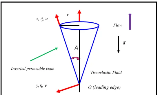
The natural convection boundary layer flow of incompressible viscoelastic fluid from a vertical permeable cone, as shown in Fig. 1, is considered. Both cone and the viscoelastic fluid are maintained initially at the same temperature and concentration. The Fourier’s law is considered for heat conduction. The influence of thermal relaxation is neglected. Viscous dissipation, thermal stratification and dispersion are also neglected. The flow is considered to be laminar and steady. The temperature and concentration of the fluid are raised instantaneously. With vertex of the cone placed at the origin, the x –coordinate is measured along the surface of the cone and the y –

coordinate is measured normal to it.The acceleration due to gravity g, acts vertically downwards. Fluid suction or injection i.e. lateral wall mass flux is imposed at the surface of the cone and the surface of the cone is held at a variable temperature and concentration proportional to the power of the distance along the slant surface i.e.

( )

1

n w T x =T_+Bd x and

( )

2 n w C x =C_+Bd x , where B,

d1, d2 are constansts and n is the power law exponent. The Jeffrey’s model accurately captures the

physical characteristic of certain polymers [27, 28]. The Cauchy stress tensor, S, of Jeffrey’s viscoelastic fluid [29] is given by:

1

,

(

)

1

p

  



= − +

=

+

+

T

I

S

S

(1)

where a dot above a quantity denotes the material time derivative, is the shear rate,  is the dynamic viscosity,  is the ratio of relaxation to retardation time and 1 is the retardation time. The

shear rate and gradient of shear rate are further defined in terms of velocity vector, V, as:

( )

. T V V



=  +  (2) .. _d . dt



=  _{ }



  (3)

With the Boussinesq approximation boundary layer approximations, the governing equations take the form:

( )

( )

0 ru rv x y   + =   ₍₄₎

(

)

(

)

2 3 2 2 3 1 2 2 2 3 * 1 cos u u u u u u u u u u v u v x y y x y x y y x y y g T T g C C A  _          ₊  ₌  ₊  ₋  ₊  ₊         + _ _         _   +_ − + − _ (5) 2 2 T T T u v x y  y  ₊  ₌     (6) 2 2 m C C C u v D x y y  ₊  ₌     ₍₇₎

The appropriate boundary conditions are:

( )

1

( )

2 0, 0, , , , 0, 0, , n n w w w At y u v V T T x T Bd x C C x C Bd x As y u v T T C C     = = = − = = + = = + →  → → → → (8)

where u and v are the velocity components in x and y direction respectively, r x

( )

=xsinA is the local radius of the truncated cone, A is the half angle of the cone, β is the coefficient of thermal expansion, β* is the coefficient of concentration expansion, T and C are temperature and concentration of the fluid respectively,  is the kinematic viscosity,  is the thermal diffusivity,

Dm is the species diffusivity, Vw is the transpiration velocity of the fluid. Vw > 0 stands for suction

i.e. mass flux removal from the boundary layer through the cone wall into the cone and Vw < 0

stands for injection i.e. blowing of fluid through the surface of the cone. Here the suffix w refers to surface conditions on the surface of the cone (wall) and ∞ refers to free stream conditions. We introduce the stream function  defined by the Cauchy-Riemann equations, ru

y



 =  and rv x



 = −

 . The mass conservation eqn. (4) is automatically satisfied. The following dimensionless

( )

( )

(

)

(

)

(

)

1/4 1/4 1/4 3 * 1 2 2 , , , , , , 2 cos Pr , , , , w x x x w w w x w m w xV y T T C C Gr rGr f Gr x T T C C g T T x A Gr C C Sc Gr De N D x T T







 

  

  



















       − −   = = = _ + _ = = − −   − − = = = = = − (9)

Here  - tangential coordinate,  - radial coordinate,  and  are the dimensionless temperature and concentration respectively, Grx - Grashof number, f - dimensionless stream function, Pr -

Prandtl number, Sc - local Schmidt number and De - Deborah number.

The resulting momentum, energy and concentration boundary layer equations take the form:

( )

(

)

(

)

2 2 1 3 1 ' ''' '' ''' 7 1 De _{2 4} '' ' '' 7 1 4 2 1 4 1 ' De ''' ' '' ' '' ' ''' '' 4 1 iv iv iv n n f f f f n n ff f f N n ff f n f f f f f f f f f f f f      _         − + _{− +}    + + + − + + + +   + + _{+ − − }     −          = _ − − _ − + − _   + _     _   (10)

(

1

)

'' 7 ' ' ' ' ' Pr 4 4 n n f f n f  f  _{  }  _   −   +   + + − = _ − _     (11)

(

1

)

'' 7 ' ' ' ' ' Sc 4 4 n n f f n f  f  _{  }  _   −   +   + + − = _ − _     (12)

The corresponding dimensionless boundary conditions are as follows:

0, 0, ' , 1, 1 , ' 0, '' 0, 0, 0 w At f f f As f f       = = = = = →  → → → → (13)

Here primes denote the differentiation with respect to . The skin-friction coefficient Cf, heat

transfer rate, Nux and mass transfer rate, Shx are defined as:

3/ 4 ''( , 0) 2 f x C f Gr =  (14) / 1/ 4 ( , 0) x x Nu Gr = −

 

(15) / 1/ 4 ( , 0) x x Sh Gr = −

 

(16) 

COMPUTATIONAL FINITE DIFFERENCES KELLER-BOX SOLUTIONS DISCUSSION

The implicit finite difference Keller-Box technique [30] is employed to solve the non-linear 8th order system of coupled boundary layer Eqns. (10) – (12) subject to boundary conditions (13). The Keller-Box technique is very popular and has been employed by many researchers that include Subba Rao et al. [31] for polymer flows from a horizontal cylinder, V.R. Prasad et al. [32] for micpolar flows,Beg et al. [33] for multi-physical magnetohydrodynamic flows, Bhuvanavijaya et al. [34] for second-grade flows, Abdul gaffar et al. [35] for third-grade model, Vasu et al. [36], Amanulla et al. [37]. The Keller-Box scheme is more efficient, powerful and accurate than the other numerical method in case of boundary layer flows which are parabolic in nature. This technique is unconditionally stable and achieves exceptional accuracy, converges quickly and provides stable numerical meshing features. The Keller-Box technique involves the following four stages:

1. Reduction of the Nth order partial differential equation system to N first order equations. 2. Finite difference discretization.

3. Quasilinearization of non-linear Keller algebraic equations. 4. Block-tridiagonal elimination of liner Keller algebraic equations.

Stage 1: Decomposition of Nth order partial differential equation system to N first order

equations

Equations (10) – (12) subject to the boundary conditions (13) are first cast as a multiple system of first order differential equations. New dependent variables are introduced:

( )

, ',

( )

, '',

( )

, ''',

( )

, , '

( )

, '

u x y = f v x y = f q x y = f s x y =  =t and g x y =with g =p (17) These denote the variables for velocity, temperature and concentration respectively. Now Equations (13) – (15) are solved as a set of eight simultaneous differential equations:

' f =u (18) ' u =v (19) ' v =q (20) ' g = p (21) ' s =t (22)

(

)

2 2 ' 7 1 1 1 3 7 ' ' 1 4 2 1 2 4 4 1 ' 4 1 v n n De n n n fv u v s Ng uq v fq q n u f De q u v f u v u q v q             + +  − + +  + − + + + − _ − + + _ + +      −       = _ − − _ − + − _   + _     _   (23) ' 7 1 Pr 4 4 t n n s f ft t n us  u t     + −   + + − = _ − _     (24) ' 7 1 4 4 p n n g f fp p n gu u p Sc       + −   + + − = _ − _     (25)

Where primes denote differentiation with respect to the variable, . In terms of the dependent variables, the boundary conditions assume the form:

0, 0, , 1, 1 , 0, 0, 0, 0 w At u v f s g As u v s g   = = = = = →  → → → → (26)

Stage 2: Finite Difference Discretization

A two-dimensional computational grid is imposed on the -η plane as depicted in Fig. 2. The stepping process is defined by:

0 0, i i 1 hj, j 1, 2,..., ,J J  =  = − + =   (27) 0 1 0, n n k_n, n 1, 2,...,N  ₌  ₌ − _{+ =} (28)

Wherekn is the - spacing and hj is the- spacing. If n j

g denotes the value of any variable at

(

 _j, n

)

, then the variables and derivatives of equations (18) – (25) at

(

1/ 2, 1/ 2

)

n j   − − are replaced by:

(

)

1/ 2 1 1 1/ 2 1 1 1 4 n n n n n j j j j j g ₋− = g +g ₋ +g − +g ₋− (29)

(

)

1/ 2 1 1 1 1 1/ 2 1 2 n n n n n j j j j j j g g g g g h  − − − − − −   _{= − + −} _    (30)

(

)

1/ 2 1 1 1 1 1/ 2 1 2 n n n n n j j j j n j g g g g g k  − − − − − −   _{= − + −} _    (31)

The finite-difference approximation of eqns. (18) – (25) for the mid-point

(

1/ 2,

)

n j  −  , are:

(

)

1 1 1/2 n n n j j j j h− f − f ₋ =u ₋ (32)

(

)

1 1 1/2 n n n j j j j h− u −u ₋ =v ₋ (33)

(

)

1 1 1/2 n n n j j j j h− v −v ₋ =q ₋ (34)

(

)

1 1 1/2 n n n j j j j h− g −g − = p − (35)

(

)

1 1 1/2 n n n j j j j h− s −s − =t − (36)

(

)

(

)(

)

(

)

(

)

(

(

)

)

(

)

(

)(

)

(

)

(

)

1 1 1 1 2 1 1 1 2 1 1 1 1 1 7 1 1 4 4 4 2 1 1 2 4 4 2 1 _{1 3 1} 1 4 1 4 4 4 1 7 1 1 2 4 4 j j j j j j j j j j j j j j j j j j j j j j j j j j j j j h h n n v v f f v v v v h h n n u u s s N g g h n h De De n n u u q q v v De n n f f q q          − − − − − − − − − − − + −   − +_ + _ + + + + +   + −   −_ + _ + + + + +   − _{ + − } − + + + _ + _ + + +   + −   − _ + _ + − +  

(

)

(

)

(

)

(

)

(

)

(

)

(

)

( )

(

)

 

1 1 1 1 1/ 2 1 1/ 2 1 1 1 1/ 2 1 1/ 2 1 1 1 1 1/ 2 1 1/ 2 1 1 /12 1 1 1 2 4 2 4 1 1 1 4 1 4 1 1 ' 1 4 1 4 j j j j n j n j j j j j j j n j n j j j j j j n n j n j j j j j j j De q q h _n h _n f v v v f f De h n De h n u q q q u u De h De n n f q q q f f R             − − − − − − − − − − − − − − − − − − − − − − − − + − − − + + + − − + + − + + + − − + − − + = + + (37)

(

)

(

)(

)

(

)

(

)(

)

(

)

(

)

(

)

(

)

 

1 1 1 1 1 1 1 1/2 1 1 1 1 1 1/2 1 1/2 1 1/2 1 2 _1/2 1 7 1 Pr 4 4 4 2 1 1 4 4 2 4 1 1 1 2 4 2 4 2 4 j j j j j j j j j j j j n j j j j j j j n j n j n j n j j j j j j j j j _j h h n n t t f f t t t t h h n n n u u s s s u u h n h n h n u s s f t t t f f R        − − − − − − − − − − − − − − − − − − − ₋ + −   − +_ + _ + + + +   − −   − +_{ } + + + +   − − − − + − + + + = (38)

(

)

(

)(

)

(

)

(

)(

)

(

)

(

)

(

)

(

)

 

1 1 1 1 1 1 1 1/2 1 1 1 1 1 1/2 1 1/2 1 1/2 1 3 _1/2 1 7 1 4 4 4 2 1 1 4 4 2 4 1 1 1 2 4 2 4 2 4 j j j j j j j j j j j j n j j j j j j j n j n j n j n j j j j j j j j j _j h h n n p p f f p p p p Sc h h n n n u u g g g u u h _n h _n h _n u g g f p p p f f R        − − − − − − − − − − − − − − − − − − − ₋ + −   − +_ + _ + + + +   − −   − +_{ } + + + +   − − − − + − + + + = (39)

1 2 n n k   = − (40)

 

( )

( )

( )

(

)

( )

( )

( )

( )

1 1 1 _{1 1} 1/ 2 1/ 2 1/ 2 1/ 2 1/ 2 2 1 1 1 _{1/ 2} 1 1 1/ 2 2 ₁ 1 1 ₁ 1 7 1 ' 1 4 4 1 1 1 2 4 1 2 1 3 1 ' 1 4 4 1 7 1 1 4 4 n n n _{n n} j j j j j n n j _j n j j n n j _j n n v f v v s Ng n n De n u uq R h De n n De v q De n n            − − − _{− −} − − − − − − − − − − − − − − − + −   +_ − _ + + + +   + − −   −_ + _ − +   = − + −   + _ − _ − +   + + −   + _ − _ +  

( )

1 1 ' n_j fq −₋                         (41)

 

1

( )

1

( )

1 ₁

( )

1 2 _{1/2 1/2 1/2} 1/2 _1/2 1 7 1 1 ' Pr 4 4 4 n n n _n n j j j j j j n n n R −₋ = −h _ t ₋− +_ + − − _ ft ₋− +t₋− − −_n  − _ us −₋ _       (42)

 

1 ₁

( )

1 ₁

( )

1 2 _1/2 1/2 _1/2 1/2 _1/2 1 7 1 1 4 4 4 n _n n _n n j j j j j j n n n R h p fp p n ug Sc    − ₋ − ₋ − − − − − −   + −   −   = − _ +_ − _ + − −_{  }       (43)

The boundary conditions are:

0 0 0, 0 1, 0 1, 0, 0, 0, 0

n n n n n n n n

J J J J

f =u = s = g = u = v = s = g = (44)

Stage 3: Quasi-linearization of Non-Linear Keller Algebraic Equations

If we assume 1 1 1 1 1 1 1 1

, , , , , , ,

n n n n n n n n

j j j j j j j j

f − u − v − q − g − p − s − t − to be known for 0 j J , then Eqns. (32) – (39) constitute a system of 8J + 8 equations for the solution of 8J + 8 unknowns

, , , , , , ,

n n n n n n n n

j j j j j j j j

f u v q g p s t , j = 0, 1, 2,…, J. This non-linear system of algebraic equations is

linearized by means of Newton’s method, as described by Takhar et al. [38].

Stage 4: Block-tridiagonal Elimination Solution of Linear Keller Algebraic Equations

The linearized system is solved by the block-elimination method, since it possesses a block-tridiagonal structure. The bock-block-tridiagonal structure generated consists of block matrices. The complete linearized system is formulated as a block matrix system, where each element in the coefficient matrix is a matrix itself, and this system is solved using the efficient Keller-box method. The numerical results are strongly influenced by the number of mesh points in both directions. After some trials in the η-direction (radial coordinate) a larger number of mesh points are selected whereas in the ξ direction (tangential coordinate) significantly less mesh points are utilized. ηmax

has been set at 10 and this defines an adequately large value at which the prescribed boundary conditions are satisfied. ξmax is set at 3.0 for this flow domain. Mesh independence is achieved in

the present computations. The numerical algorithm is executed in MATLAB on a PC. The method demonstrates excellent stability, convergence and consistency, as elaborated by Keller [30].

RESULTS AND DISCUSSION

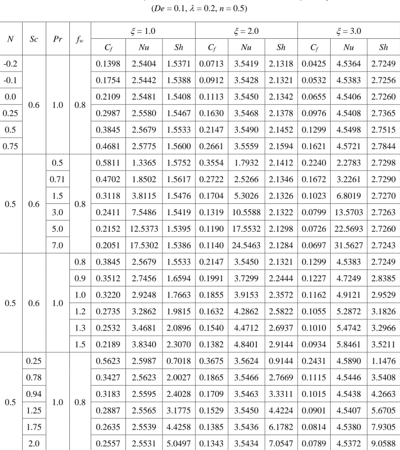
The influence of various engineering parameters of an incompressible viscoelastic Jeffrey’s fluid past a vertical permeable cone with ramped wall temperature and concentration is analysed numerically. Comprehensive results are obtained and are presented in Tables 1 - 2 and

Figs. 2 - 10. The influences of different thermophysical parameters, viz., De, , n, N, Pr, Sc, fw, 

are examined. The prescribed default parameter values are: De = 0.1,  = 0.2, n = 0.5, N = 0.5, Pr = 1.0, Sc = 0.6, fw = 0.8. Table 1 presents the numerical values of heat transfer rate and are

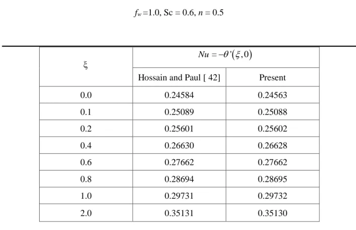
compared with Hossain and Paul [38] for different values of  with Pr = 0.1, N = 0.5, fw = 1.0, Sc

= 0.6 when De = 0.0 = λ (Newtonian case) and are found to be in excellent agreement. Table 2

provides the results for the influence of Buoyancy ratio parameter (N), Schmidt number (Sc), Prandtl number (Pr) and suction/injection parameter (fw) on skin friction (Cf), heat transfer rate

(Nu) and mass transfer rate (Sh) for different values of . An increase in N is seen to increase skin friction, heat transfer rate and mass transfer rate. A significant reduction in Cf is observed with

increasing Sc. A slight decrease in Nu is seen with increasing values of Sc whereas Sh is enhanced. Increasing Sc implies a decrease in species mass diffusivity. For Sc < 1, the species diffusion rate exceeds the momentum diffusion rate and vice versa for Sc > 1 And for Sc = 1, both diffusion rates are the same and the momentum and concentration boundary layer thicknesses are the same in the regime. Nu is greater with larger Pr values and lower with smaller Pr, as presented in Table 2. But

Cf and Sh are lowered for an increase in Pr. The parameter Pr indicates the ratio of momentum

diffusion to the thermal diffusion. For Pr > 1, momentum diffusion dominates the heat diffusion and vice versa for Pr < 1. Higher Pr values implies to a lower thermal conductivity of the polymer fluid. As Pr is the only non-dimensional parameter that categorizes thermofluid properties, Pr

should be varies in order to generalize the solutions of denser fluids such as water-based solvents and very low-density spray paints [39]. With greater Pr, velocity reduces and hence skin friction also decreases. Thereby increases the corresponding momentum boundary layer thickness. If Pr < 1 then the thermal diffusion rate compared with momentum diffusion rate will be greater. A lower

Prandtl number (Pr = 0.71 i.e. gas) implies that the fluid will possess higher thermal conductivity

(and an associated thicker thermal boundary layer structure) so that heat can diffuse away from the fluid to the cone surface faster than for higher Prandtl number fluid (Pr = 7.0 i.e. liquids associated with thinner boundary layers). Therefore, lower Prandtl number fluids will achieve significantly larger temperatures in the boundary layer. Higher Prandtl number fluids possess lower thermal conductivities causing less thermal energy to be diffused from the fluid to the cone surface and resulting in lower temperatures. The heat transfer rate from the cone surface to the fluid is therefore greater with larger Prandtl number and lower with smaller Prandtl number, as testified to in Table 2. Increasing fw is seen to reduce skin friction and heat transfer rate whereas mass transfer rate is

enhanced.

Figs. 2(a) – 2(c) illustrates the impacts of De on velocity

( )

f ' , temperature

( )



and concentration

( )



distributions. Velocity (fig. 2a) is reduced significantly with an increase in De

values. De arises in connection with higher order derivatives in the momentum boundary layer eqn. (10). Hence the parameter De expends a significant influence on shearing characteristics of the polymer flows. From the definition, De is the ratio of characteristic time to the time scale of deformation. For a fixed value of the characteristic time, there may be different values of the time scale of deformation and hence there can be various values for De in case of the same polymer. For De > 1.0, elasticity dominates and for De < 0.5, viscosity dominates. For high values of De, the polymers act highly oriented in one direction, stretched and the fluid behaves as purely elastic. However, in case of small De values, the polymer acts as a simple viscous fluid. The figs. 2(b) and 2(c) shows a very slight increase in temperature and concentration with an increase in De values. Similar trends were observed by Hayat et al. [40]. De arises in connection with many higher order derivatives in the momentum boundary layer Eqn. (10). Therefore, it is intimately associated with the shearing characteristic of the polymer flow. In polymer flows, for higher De values the polymer become highly oriented in one direction and stretched, and this occurs when the polymer takes longer to relax in comparison to the deforming rate of the flow. Further from the cone surface it is observed that there is a slight increase in the velocity i.e. the flow is accelerated with increasing

De. With greater distance from the solid boundary, the polymer is assisted in flowing even with higher elastic effects. Clearly the responses in the near-wall region and far-field region are very different. Though De dose not arise in the thermal boundary layer Eqn. (11), there is a strong

coupling of this equation with the momentum equation. The momentum Eqn. (10) strongly couples the momentum field to the temperature field. With greater elastic effects, it is anticipated that thermal conduction plays a greater role in hear transfer in the polymer.

Figs. 3(a) – 3(c) depicts the effects of the ratio of relaxation to retardation time,  on

velocity

( )

f ' , temperature

( )



and concentration

( )



distributions. Clearly, from fig. 3(a) we can observe a significant increase in linear velocity with greater  values. However, the temperature and concentration as seen figs. 3(b) & 3(c) respectively decrease slightly with greater

values. Therefore, the flow of polymer is considerably accelerated with an increase in relaxation time (or decrease in retardation time). The parameter , arises in many terms in the momentum boundary layer eqn. (10). Therefore, this parameter exerts a tangential influence on the flow characteristics. Increasing relaxation time increases the momentum boundary layer whereas decreases both thermal and mass diffusion. Therefore, the flow of polymer is considerably accelerated with an increase in relaxation time (or decrease in retardation time). For greater relaxation times, the thermal boundary layer thickness is reduced. Whereas with greater relaxation times, the momentum boundary layer thickness is decreased only near the cone surface whereas further away it is enhanced as the flow is strongly accelerated in this regime.

Figs. 4(a) – 4(c) presents the influence of power-law index n on velocity

( )

f ' , temperature

( )



and concentration

( )



distributions. It is observed that as n increases, the linear velocity of the fluid (fig. 4(a)) decreases considerably. Fig. 4(b) presents the responses of n on temperature profiles. The temperature profiles are decreased significantly with an increase in n. Also, the concentration is decreased slightly (fig.4(c)) with the increasing values of n. The non-isothermal index relates to the variation in cone surface i.e. wall temperature and concentration. For n > 0, the wall temperature increase with distance from the leading edge and for n < 0, wall temperature decreases. The wall is isothermal if n = 0. The non-isothermal index arises in the primitive wall temperature and concentration of Eqn. (8) and features in numerous terms in Eqns. (13) – (15). As the wall temperature increases, the relative difference of wall and fluid temperature increases. Non-isothermal wall index is clearly an important parameter adjusting the thermal flow characteristics. Increasing positive non-isothermal index therefore manifests in a deceleration in boundary layer flow and a corresponding increase in momentum (hydrodynamic) boundary layer thickness and a reduction in thermal boundary layer thickness. Note that only positive non-isothermal index is

considered (the case of n < 0, physically represents progressive cooling of the cone surface from the leading edge and this is not relevant here).

Figs. 5(a) – 5(c) illustrates the effects for velocity

( )

f ' , temperature

( )



and concentration

( )



for various values of N. An increasing N is seen to found to significantly enhance the velocity, whereas, a significant decrease in both temperature and concentration is seen to for various values of N.

Figs. 6(a) – 6(c) illustrates the profiles for velocity

( )

f ' , temperature

( )



and concentration

( )



for different values of fw. Increasing fw strongly decelerates the flow i.e. velocity

is reduced. Temperatures are also decreased, as observed in fig. 6b with increasing values of fw.

The boundary layer thickness is reduced and suction causes the boundary layer to adhere closer to the wall. Temperatures are also decreased, as observed in fig. 6b with increasing values of fw in the boundary layer regime and strongly decrease thermal boundary layer thickness. There is a strong reduction in concentration values with increasing fwvalues, as shown in fig. 6c. As seen in

all the graphs, only the case of wall suction are studied i.e. fw > 0. Although boundary layer separation has not been identified in the present regime, suction has been shown to delay this effect in certain viscoelastic cone flow problems. Greater suction evidently aids in adherence of the momentum boundary layer to the cone surface which depresses flow momentum and reduces velocity magnitudes. However, it done not induce back flow since magnitudes are always positive. The thickening of the momentum boundary layer simultaneously inhibits heat diffusion which leads to a plummet in temperature i.e cooler boundary layers and this is also of relevance to optimized thermal processing systems.

Figs. 7(a) – 7(c) presents the effects of velocity

( )

f ' , temperature

( )



and concentration

( )



for different values of . The parameter  also incorporates the local Grashof number, Grx

and can be seen as a free convection parameter as discussed in [41]. Clearly, it is observed that the fluid velocity reduces with the increasing values of . The location of the flow moves further along the cone surface from the apex. And hence the buoyancy forces increases as the momentum diffusion suppress, leading to a decrease in the flow and a thicker boundary layer structure. Also, it is seen that the temperature and concentration profiles are also reduced for increasing values of

is increased, more warm fluid is taken away and thus the thermal boundary layer thickness decreases. The tangential (streamwise) coordinate is an inverse function of local Grashof number and is therefore inversely proportional to thermal buoyancy force in the regime. Therefore with larger  values, buoyancy force is progressively reduced which assists in promoting heat transfer but counteracts the momentum development.

Figs. 8(a) – 8(c) illustrates the profiles for De on skin friction coefficient, heat transfer rate and mass transfer rate at the cone surface. The dimensionless skin friction is reduced for increasing values of De, owing to the increase in elastic effects which also serve to reduce the boundary layer thickness as the flow decelerates. Also, the heat transfer rate and mass transfer rate are reduced substantially with increasing De values. Therefore, momentum, thermal and species diffusion inhibit with increasing elasticity effect. A decrease in heat transfer rate at the wall implies less heat is convected from the fluid regime to the cone thereby heating the boundary layer. The mass transfer rate decreases with increasing De values and furthermore plummets with further distance from the lower stagnation point.

Figs. 9(a) – 9(c) depicts the response to , on skin friction coefficient, heat transfer rate and mass transfer rate at the cone surface. A significant increases in the skin friction is observed at the cone surface for increasing values of . Also, a strong elevation in shear stress is observed with increasing  values. Hence, the flow accelerates strongly along the cone surface away from the lower stagnation point. Heat and mass transfer rates also increase substantially with increasing

 values. As the relaxation time increases i.e., as the retardation time decreases, faster the polymer flows and results in the acceleration in boundary layer flow and heat and species concentration are diffused. Figs. 10(a) – 10(c) presents the effects of the power-law exponent, n, on the skin friction coefficient, heat transfer rate and mass transfer rate at the cone surface. The skin friction is decreased with increasing values of n. Conversely, the heat transfer rate is increased with increasing n as shown in fig. 10(b). Likewise, the mass transfer rate is also increased significantly for n values as shown in fig. 10(c). With greater wall temperature further from the leading edge, the relative difference of wall and fluid temperature is increased. This induces greater heat transfer from the wall (cone surface) into the boundary layer and boosts Nusselt number. The elevation in thermal diffusion counter-acts the momentum diffusion which leads to a depression in surface shear stresses and therefore skin friction.

CONCLUSIONS

A non-similar mathematical model has been presented for buoyancy-driven, laminar convection boundary layer flows of viscoelastic Jeffrey’s fluid from a vertical permeable cone with ramped wall temperature and concentration. The transformed boundary layer conservation equations with prescribed boundary conditions have been solved using the finite difference Keller-Box technique. A comprehensive assessment of different thermophysical quantities is discussed graphically. Excellent convergence and stable characteristics are demonstrated by the Keller-box scheme. The present numerical code is able to solve nonlinear boundary layer equations very efficiently and shows an excellent promise in simulating transport phenomena in other non-Newtonian fluids. It is therefore presently being employed to study viscoplastic fluids which also represent other chemical engineering working fluids in curved geometrical systems.

REFERENCES

[1] T. F. Irvine, J. Karni, Non-Newtonian fluid flow and heat transfer, Handbook of Single-Phase Convective heat transfer, Chapter 20, Wiley New York, 20.1 – 20.57, 1987.

[2] Alessandra Borrelli, Giulia Giantesio, Maria Cristina Patria, MHD Oblique stagnation-point flow of a micropolar fluid, Applied Mathematical Modelling, Vol. 36, Issue 9, pp.3949-3970, 2012. [3] Azad Hussain, Anwar Ullah, Boundary layer flow of a Walter’s B fluid due to a stretching cylinder with temperature dependent viscosity, Alexandria Engineering Journal, Vol. 55, Issue 4, pp.3073-3080, 2016.

[4] S. Abdul Gaffar, V. Ramachandra Prasad, E. Keshava Reddy, Computational study of Jeffrey’s non-Newtonian fluid past a semi-infinite vertical plate with thermal radiation and heat generation/absorption, Ain Shams Engineering Journal, Vol. 8, Issue 2, pp.277-294, 2017. [5] A. Subba Rao, C.H. Amanulla, N. Nagendra, O. Anwar Bég, A. Kadir, Hydromagnetic flow and heat transfer in a Williamson Non-Newtonian fluid from a Horizontal circular cylinder with Newtonian Heating, Int. J. Appl. Comput. Math, Vol. 3, Issue 4, pp.3389-3409, 2017.

[6] Ramachandra Prasad V., S. Abdul Gaffar and O. Anwar Bég, Non-Similar computational solutions for free convection boundary layer flow of a nanofluid from an isothermal sphere in a Non-Darcy porous medium, J. Nanofluids, Vol. 4, No. 2, pp.203-213, 2015.

[7] Huicui Li, Yongjun Jian, Dispersion for periodic electro-osmotic flow of Maxwell fluid through a microtube, Int. J. Heat and Mass Transfer, Vol. 115, Part A, pp.703-713, 2017.

[8] S. Abdul Gaffar, V. Ramachandra Prasad, O. Anwar Bég, Computational study of non-Newtonian Eyring-Powell fluid from a vertical porous plate with Biot number effects, J. Braz. Soc. Mech. Sci. Eng., Vol. 39, Issue 7, pp.2747-2765, 2017.

[9] S. Abdul Gaffar, V. Ramachandra Prasad, E. Keshava Reddy, Computational Study of MHD free convection flow of non-Newtonian Tangent Hyperbolic fluid from a vertical surface in porous media with Hall/Ionslip current and Ohmic dissipation, Int. J. App. Comp. Math., Vol. 3, Issue 2, pp.859-890, 2017.

[10] R. Mehmood, S. Rana, S. Nadeem, Transverse thermophoretic MHD Oldroyd-B fluid with Newtonian heating, Results in Physics, 8, pp.686-693, 2018.

[11] Zhi-Yong Xie, Yong-Jun Jian, Rotating electromagnetohydrodynamic flow of power-law fluids through a microparallerl channel, Colloids and Surfaces A: Physicochemical and Engineering Aspects, Vol. 529(20), pp.334-345, 2017.

[12] Katini Ahmad, Zahir Hanouf and Anuar Ishak, Mixed convection Jeffrey fluid flow over an exponentially stretching sheet with magnetohydrodynamic effect, AIP Advances, 6, 035024 (2016); doi:10.1063/1.4945401.

[13] Muhammad Saqib, Farhad Ali, Ilyas Khan, Nadeem Ahmad Sheik, Syed Aftab Alam Jan, Samiulhaq, Exact solutions for free convection flow of generalized Jeffrey fluid: A Caputo-Fabrizio fractional model, Alex. Eng. J., 2017. http://doi.org/10.1016/j.aej.2017.03.017.

[14] Odelu Ojjela, Adigoppula Raju, Pravin Kashyap Kambhatla, Influence of thermophoresis and induced magnetic field on chemically reacting mixed convective flow of Jeffrey fluid between porous parallel plates, J. Molecular Liquids, Vol.232, pp. 195-206, 2017.

[15] T. Hayat, T. Muhammad, Meraj Mustafa, Ahmed Alsaedi, Three-dimensional flow of Jeffrey fluid with Cattaneo-Christov heat flux: An application to non-Fourier heat flux theory, Chinese J. of Physics, 2017. http://doi.org/10.1016/j.cjph.2017.03.014.

[16] M.M. Bhatti, R. Ellahi, A. Zeeshan, Study of variable magnetic field on the peristaltic flow of Jeffrey fluid in a non-uniform rectangular duct having compliant walls, J. Molecular Liquids, Vol. 222, pp. 101-108, 2016.

[17] Siti Nur Haseela Izani and Anati Ali, Mixed convective boundary layer flow of a dusty Jeffrey fluid over an exponentially stretching sheet, Int. Conference on Mathematics, Engineering and Industrial Applications 2016 (ICoMEIA2016), AIP Conf. Proc., 1775, 030057-1 – 030057-9, 2016. DOI:10.1063/1.4965177.

[18] Hayat T., Sumaria Qayyum, Maria Imtiaz, Ahmed Alsaedi, Impact of Cattaneo-Christov Heat Flux in Jeffrey Fluid flow with Homogeneous-Heterogeneous Reactions, PLoS ONE, 11(2):e0148662. doi:10.1371/journal.pone.0148662.

[19] Hayat T., Asad Sadia and Alsaedi A., Analysis for flow of Jeffrey fluid with nanoparticles,

Chinese Physics B, Vol. 24, No. 4, 044702, 2015. https://doi.org/10.1088/1674-1056/24/4/044702. [20] P.V. Satya Narayana, D. Harish Babu, Numerical study of MHD heat and mass transfer of a Jeffrey fluid over a stretching sheet with chemical reaction and thermal radiation, J. Taiwan Institute of Chemical Engineers, Vol.59, pp.18-28, 2016.

[21] K. Javaherdeh, Mehrzad Mirzaei Nejad, M. Moslemi, Natural convection heat and mass transfer in MHD fluid flow past a moving vertical plate with variable surface temperature and concentration in a porous medium, Eng. Sci. Tech., an Int. J., Vol. 18, Issue 3, pp.423-431, 2015. [22] Rajnessh Kumar, Ibrahim A. Abbas, Veena Sharma, A numerical study of free convection heat and mass transfer in a Rivlin-Ericksen viscoelastic flow past an impulsively started vertical plate with variable temperature and concentration, Int. J. Heat and Fluid Flow, Vol. 44, pp.258-264, 2013.

[23] Farhad Ali, Madeha Gohar, Iiyas Khan, MHD flow of water-based Brinkman type nanofluid over a vertical plate embedded in a porous medium with variable surface velocity, temperature and concentration, J. Molecular Liquids, Vol. 233, pp.412-419, 2016.

[24] Hari R. Kataria, Harshad R. Patel, Effect of themo-diffusion and parabolic motion of MHD second grade fluid flow with ramped wall temperature and ramped surface concentration,

Alexandria Engineering Journal, 2016. http://doi.org/10.1016/j.aej.2016.11.014.

[25] R. Kandasamy, Abd. Wahid, B. Md. Raj, Azme B. Khamis, Effects of chemical reaction, heat and mass transfer on boundary layer flow over a porous wedge with heat radiation in the presence of suction or injection, Theroret. Appl. Mech., Vol. 33, No. 2, pp.123-148, Belgrade 2006. [26]S. Hussain and M.A. Hossain, Natural convection flow from a vertical permeable flat plate with variable surface temperature and species concentration, Engineering Computations, Vol. 17, Issue 7, pp.789-812, 2000.

[27] Bird, R.B., Armstrong, R.C. and Hassager, O., Dynamics of Polymeric Liquids. Volume 1: Fluid Mechanics, Vol. 1, 2nd Edition, Wiley Interscience, New York, USA (1987).

[28] Larson, R.G., Constitutive Equations for Polymer Melts and Solutions, Series in Chemical Engineering, Butterworths, Boston (1988).

[29] Nadeem S, Akbar N S., Peristaltic flow of a Jeffrey fluid with variable viscosity in an asymmetric channel, Z Naturforsch A, 2009; 64a:713–22.

[30] H.B. Keller, Numerical methods in boundary-layer theory, Ann. Rev. Fluid Mech. 10, 417-433 (1978).

[31] A. Subba Rao, V. Ramachandra Prasad, P. Rajendra, M. Sasikalam, O. Anwar Bég, Numerical study of non-Newtonian polymeric boundary layer flow and heat transfer from a permeable horizontal isothermal cylinder, Frontiers in Heat and Mass Transfer, Issue 9, No. 2, 2017.

[32] V. Ramachandra Prasad, S. Abdul Gaffar and O. Anwar Bég, Heat and Mass transfer of Nanofluid from a horizontal cylinder to micropolar fluid, J. Thermophysics and Heat Transfer, vol. 29, No. 1, pp.127-139, 2015.

[33] O. Anwar Bég, Numerical methods for multi-physical magnetohydrodynamics, Chapter 1, pp. 1-112, New Developments in Hydrodynamics Research, Nova Science, New York, September

(2012).

[34] R. Bhyvanavijaya, V. Ramachandra Prasad, B. Mallikarjuna and O. Anwer Bég, Natural convective heat transfer flow a non-Newtonian second-grade fluid past an isothermal sphere,

Computational Thermal Sciences: An Int. J., Vol. 6, Issue 5, pp.451-460, 2014.

[35] S. Abdul Gaffar, V. Ramachandra Prasad, O. Anwar Bég, Md. H. Hidayathullah Khan, K. Venkatadri, Radiative and magnetohydrodynamics flow of third-grade viscoelastic fluid past an isothermal inverted cone in the presence of heat generation/ absorption, J. Braz. Soc. Mech. Sci. Eng.., 2018. https://doi.org/10.1007/s40430-018-1049-0.

[36] B. Vasu, V.R. Prasad, O. Anwar Bég, A. Aziz, Numerical analysis of magnetohydrodynamic nonlinear convection heat and mass transfer form a sphere in non-Darcian variable-porosity medium, Int. J. Appl. Math. And Mech., Vol. 6, Issue 17, 2010.

[37] Ch. Amanulla, N. Nagendra, M. Suryanarayana Reddy, Numerical simulation of slip influence of electric conducting viscoelastic fluid past an isothermal cylinder, Frontiers in Heat and Mass Transfer, Vol. 10, Issue 10, 2018.

[38] Takhar, H.S., Bég, O. Anwar and M. Kumari, Computational analysis of coupled radiation convection dissipative flow in a porous medium using the Keller-Box implicit difference scheme,

Int. J. Energy Research, 22,141-159 (1998).

[39] Rohsenow, W.M.; Hartnett, J.P.; Ganic, E.N., Handbook of Heat Transfer Fundamentals, Mac-Graw-Hill, New York, 2nd edn (1985).

[40] Hayat T., Shehzad. S.A., Qasim M. and Obaidat. S., Radiative flow of Jeffery fluid in a porous medium with power law heat flux and heat source, Nuclear Engineering and Design, 243, 15-19 (2012).

[41] R. S. R. Gorla, A. Slaouti, H.S. Takhar, Free convection in micropolar fluids over a uniformly heated vertical plate, Int. J. Numerical Methods for Heat & Fluid Flow, 8, 504 – 518, (1988). [42] M. A. Hossain, S.C. Paul, Free convection from a vertical permeable circular cone with non-uniform surface temperature, Acta Mechanica, 151, pp. 103-114, (2001).

TABLES

Table 1: Values of Nu = − '

( )

, 0 for various values of with De = 0.0 = λ, Pr = 0.1, N = 0.5,

fw =1.0, Sc = 0.6, n = 0.5

 Nu =− '

( )

, 0

Hossain and Paul [ 42] Present

0.0 0.24584 0.24563 0.1 0.25089 0.25088 0.2 0.25601 0.25602 0.4 0.26630 0.26628 0.6 0.27662 0.27662 0.8 0.28694 0.28695 1.0 0.29731 0.29732 2.0 0.35131 0.35130

Table 2: Values of Cf, Nu and Sh for various values of N, Pr, Sc, fw and  (De = 0.1,  = 0.2, n = 0.5) N Sc Pr fw = 1.0  = 2.0  = 3.0 Cf Nu Sh Cf Nu Sh Cf Nu Sh -0.2 0.6 1.0 0.8 0.1398 2.5404 1.5371 0.0713 3.5419 2.1318 0.0425 4.5364 2.7249 -0.1 0.1754 2.5442 1.5388 0.0912 3.5428 2.1321 0.0532 4.5383 2.7256 0.0 0.2109 2.5481 1.5408 0.1113 3.5450 2.1342 0.0655 4.5406 2.7260 0.25 0.2987 2.5580 1.5467 0.1630 3.5468 2.1378 0.0976 4.5408 2.7365 0.5 0.3845 2.5679 1.5533 0.2147 3.5490 2.1452 0.1299 4.5498 2.7515 0.75 0.4681 2.5775 1.5600 0.2661 3.5559 2.1594 0.1621 4.5721 2.7844 0.5 0.6 0.5 0.8 0.5811 1.3365 1.5752 0.3554 1.7932 2.1412 0.2240 2.2783 2.7298 0.71 0.4702 1.8502 1.5617 0.2722 2.5266 2.1346 0.1672 3.2261 2.7290 1.5 0.3118 3.8115 1.5476 0.1704 5.3026 2.1326 0.1023 6.8019 2.7270 3.0 0.2411 7.5486 1.5419 0.1319 10.5588 2.1322 0.0799 13.5703 2.7263 5.0 0.2152 12.5373 1.5395 0.1190 17.5532 2.1298 0.0726 22.5693 2.7260 7.0 0.2051 17.5302 1.5386 0.1140 24.5463 2.1284 0.0697 31.5627 2.7243 0.5 0.6 1.0 0.8 0.3845 2.5679 1.5533 0.2147 3.5450 2.1321 0.1299 4.5383 2.7249 0.9 0.3512 2.7456 1.6594 0.1991 3.7299 2.2444 0.1227 4.7249 2.8385 1.0 0.3220 2.9248 1.7663 0.1855 3.9153 2.3572 0.1162 4.9121 2.9529 1.2 0.2735 3.2862 1.9815 0.1632 4.2862 2.5822 0.1055 5.2872 3.1826 1.3 0.2532 3.4681 2.0896 0.1540 4.4712 2.6937 0.1010 5.4742 3.2966 1.5 0.2189 3.8340 2.3070 0.1382 4.8401 2.9144 0.0934 5.8461 3.5211 0.5 0.25 1.0 0.8 0.5623 2.5987 0.7018 0.3675 3.5624 0.9144 0.2431 4.5890 1.1476 0.78 0.3427 2.5623 2.0027 0.1865 3.5466 2.7669 0.1115 4.5446 3.5408 0.94 0.3183 2.5595 2.4028 0.1709 3.5463 3.3311 0.1015 4.5438 4.2663 1.25 0.2887 2.5565 3.1775 0.1529 3.5450 4.4224 0.0901 4.5407 5.6705 1.75 0.2635 2.5539 4.4258 0.1385 3.5436 6.1782 0.0814 4.5380 7.9305 2.0 0.2557 2.5531 5.0497 0.1343 3.5434 7.0547 0.0789 4.5372 9.0588

FIGURES

Fig. 1 Geometric illustration of problem

Fig. 2: Keller box computational cell

g

O (leading edge) y,, v

x, , u

Inverted permeable cone

A

r

Viscoelastic Fluid Flow



 Keller box cell

Stepping direction directionoelastic

0 0.04 0.08 0.12 0.16 0 4 8 12 De = 0.01, 0.15, 0.5, 1, 2, 3

Fig. 2(a) Influence of De on Velocity Profiles

 = 0.5, Pr = 1.0, N = 0.5, n= 0.5, Sc = 0.6, = 1.0, f_w= 0.8 f ' 0 0.2 0.4 0.6 0.8 1 0 1 2 3 4 De = 0.01, 0.15, 0.5, 1, 2, 3

Fig. 2(b) Influence of De on TemperatureProfiles

 = 0.5, Pr = 1.0, N = 0.5, n= 0.5, Sc = 0.6, = 1.0, f_w= 0.8  0 0.2 0.4 0.6 0.8 1 0 2 4 6 De = 0.01, 0.15, 0.5, 1, 2, 3

Fig. 2(c) Influence of De on Concentration Profiles



= 0.5, Pr = 1.0, N = 0.5, n= 0.5, Sc = 0.6, = 1.0, f_w= 0.8

0 0.05 0.1 0.15 0.2 0.25 0 2 4 6 = 0, 2, 5, 10, 15, 20

Fig. 3(a) Influence of on Velocity Profiles

 De = 0.1, Pr = 1.0, N = 0.5, n= 0.5, Sc = 0.6, = 1.0, f_w= 0.8 f ' 0 0.2 0.4 0.6 0.8 1 0 1 2 3 = 0, 2, 5, 10, 15, 20

Fig. 3(b) Influence of on Temperature Profiles

 De = 0.1, Pr = 1.0, N = 0.5, n= 0.5, Sc = 0.6, = 1.0, f_w= 0.8  0 0.2 0.4 0.6 0.8 1 0 1 2 3 4 5 = 0, 2, 5, 10, 15, 20

Fig. 3(c) Influence of on Concentration Profiles



De = 0.1, Pr = 1.0, N = 0.5, n= 0.5, Sc = 0.6, = 1.0, f_w= 0.8

0 0.05 0.1 0.15 0 2 4 6 8 n= 0, 0.4, 0.8, 1, 1.5, 2

Fig. 4(a) Influence of non Velocity Profiles

 De = 0.1, = 0.1, Pr = 1.0, N = 0.5, Sc = 0.6, = 1.0, f_w= 0.8 f ' 0 0.2 0.4 0.6 0.8 1 0 1 2  3 4  n= 0, 0.4, 0.8, 1, 1.5, 2

Fig. 4(b) Influence of non Temperature Profiles

De = 0.1, = 0.1, Pr = 1.0, N = 0.5, Sc = 0.6, = 1.0, f_w= 0.8 0 0.2 0.4 0.6 0.8 1 0 1 2 3 4 5   n= 0, 0.4, 0.8, 1, 1.5, 2

Fig. 4(c) Influence of non Concentration Profiles

0 0.05 0.1 0.15 0 2 4 6 f '  N= -0.2. -0.1, 0, 0.25, 0.5, 0.75

Fig. 5(a) Influence of Non Velocity Profiles

De = 0.1, = 0.1, Pr = 1.0, n= 0.5, Sc = 0.6, = 1.0, f_w= 0.8 0 0.2 0.4 0.6 0.8 1 0 1 2 3   N= -0.2. -0.1, 0, 0.25, 0.5, 0.75

Fig. 5(b) Influence of Non Temperature Profiles

De= 0.1, = 0.1, Pr = 1.0, n= 0.5, Sc = 0.6, = 1.0, f_w= 0.8 0 0.2 0.4 0.6 0.8 1 0 1 2 3 4 5   N= -0.2. -0.1, 0, 0.25, 0.5, 0.75

Fig. 5(c) Influence of Non Concentration Profiles

0 0.04 0.08 0.12 0 2 4 6 8 f '  f_w= 0.8, 0.9, 1, 1.2, 1.3, 1.5

Fig. 6(a) Influence of f_won Velocity Profiles

De = 0.1, = 0.1, Pr = 1.0, n= 0.5, Sc = 0.6, N = 0.5, = 1.0 0 0.2 0.4 0.6 0.8 1 0 1 2 3 4   f_w= 0.8, 0.9, 1, 1.2, 1.3, 1.5

Fig. 6(b) Influence of f_won Temperature Profiles

De = 0.1, = 0.1, Pr = 1.0, n= 0.5, Sc = 0.6, N = 0.5, = 1.0 0 0.2 0.4 0.6 0.8 1 0 1 2 3 4 5   f_w= 0.8, 0.9, 1, 1.2, 1.3, 1.5

Fig. 6(c) Influence of f_won Concentration Profiles

0 0.06 0.12 0.18 0 2 4 6 8 f '  = 0, 0.5, 1, 1.5, 2, 3

Fig. 7(a) Influence of on Velocity Profiles

De = 0.1, = 0.1, Pr = 1.0, n= 0.5, Sc = 0.6, N = 0.5, f_w= 0.8 0 0.2 0.4 0.6 0.8 1 0 1 2 3 4   = 0, 0.5, 1, 1.5, 2, 3

Fig. 7(b) Influence of on Temperature Profiles

De = 0.1, = 0.1, Pr = 1.0, n= 0.5, Sc = 0.6, N = 0.5, f_w= 0.8 0 0.2 0.4 0.6 0.8 1 0 1 2 3 4 5   = 0, 0.5, 1, 1.5, 2, 3

Fig. 7(c) Influence of on Concentration Profiles

0.2 0.4 0.6 0.8 1 0 0.02 0.04 0.06 0.08 0.1 De = 0.01, 0.15, 0.5, 1, 2, 3

Fig. 8(a) Influence of De on Skin Friction

 = 0.5, Pr = 1.0, N = 0.5, n= 0.5, Sc = 0.6, f_w= 0.8 Cf 1.4 1.6 1.8 2 0 0.02 0.04 0.06 0.08 0.1 De = 0.01, 0.15, 0.5, 1, 2, 3

Fig. 8(b) Influence of De on Local Nusselt number

 = 0.5, Pr = 1.0, N = 0.5, n= 0.5, Sc = 0.6, f_w= 0.8 N u 0.6 0.8 1 1.2 0 0.02 0.04 0.06 0.08 0.1 De = 0.01, 0.15, 0.5, 1, 2, 3

Fig. 8(c) Influence of De on Local Sherwood number



= 0.5, Pr = 1.0, N = 0.5, n= 0.5, Sc = 0.6, f_w= 0.8

0.2 0.4 0.6 0.8 0 0.02 0.04 0.06 0.08 0.1 Cf De = 0.1, Pr = 1.0, N = 0.5, n= 0.5, Sc = 0.6, f_w= 0.8

Fig. 9(a) Influence of on Skin Friction

 = 0, 2, 5, 10, 15, 20 1.5 1.7 1.9 2.1 0 0.02 0.04 0.06 0.08 0.1 De = 0.1, Pr = 1.0, N = 0.5, n= 0.5, Sc = 0.6, f_w= 0.8

Fig. 9(b) Influence of on Local Nusselt number

 = 0, 2, 5, 10, 15, 20 N u 0.8 1 1.2 1.4 0 0.02 0.04 0.06 0.08 0.1 S h De = 0.1, Pr = 1.0, N = 0.5, n= 0.5, Sc = 0.6, f_w= 0.8

Fig. 9(c) Influence of on Local Sherwood number

 = 0, 2, 5, 10, 15, 20

0 0.25 0.5 0.75 1 0 0.02 0.04 0.06 0.08 0.1 Cf n= 0, 0.4, 0.8, 1, 1.5, 2 De = 0.1, = 0.1, Pr = 1.0, N = 0.5, Sc = 0.6, f_w= 0.8

Fig. 10(a) Influence of non Skin Friction

 0 1 2 3 0 0.02 0.04 0.06 0.08 0.1 N u n= 0, 0.4, 0.8, 1, 1.5, 2 De = 0.1, = 0.1, Pr = 1.0, N = 0.5, Sc = 0.6, f_w= 0.8

Fig. 10(b) Influence of non Local Nusselt number

 0 0.5 1 1.5 2 0 0.02 0.04 0.06 0.08 0.1 S h n= 0, 0.4, 0.8, 1, 1.5, 2 De = 0.1, = 0.1, Pr = 1.0, N = 0.5, Sc = 0.6, f_w= 0.8

Fig. 10(c) Influence of non Local Sherwood number