Optimization Foundations of Reinforcement Learning

(1)

Jalaj Bhandari

Submitted in partial fulfillment of the requirements for the degree of

Doctor of Philosophy under the Executive Committee of the Graduate School of Arts and Sciences

COLUMBIA UNIVERSITY

(2)

(3)

Abstract

Optimization Foundations of Reinforcement Learning Jalaj Bhandari

Reinforcement learning (RL) has attracted rapidly increasing interest in the machine learn-ing and artificial intelligence communities in the past decade. With tremendous success already demonstrated for Game AI, RL offers great potential for applications in more complex, real world domains, for example in robotics, autonomous driving and even drug discovery. Although re-searchers have devoted a lot of engineering effort to deploy RL methods at scale, many state-of-the art RL techniques still seemmysterious- with limited theoretical guarantees on their behaviour in practice.

In this thesis, we focus on understanding convergence guarantees for two key ideas in re-inforcement learning, namely Temporal difference learning and policy gradient methods, from an optimization perspective. In Chapter 2, we provide a simple and explicit finite time analy-sis of Temporal difference (TD) learning with linear function approximation. Except for a few key insights, our analysis mirrors standard techniques for analyzing stochastic gradient descent algorithms, and therefore inherits the simplicity and elegance of that literature. Our convergence results extend seamlessly to the study of TD learning with eligibility traces, known as TD(𝜆), and to Q-learning for a class of high-dimensional optimal stopping problems.

In Chapter 3, we turn our attention to policy gradient methods and present a simple and general understanding of their global convergence properties. The main challenge here is that even for simple control problems, policy gradient algorithms face non-convex optimization problems and

(4)

are widely understood to converge only to a stationary point of the objective. We identify structural properties – shared by finite MDPs and several classic control problems – which guarantee that despite non-convexity, any stationary point of the policy gradient objective is globally optimal. In the final chapter, we extend our analysis for finite MDPs to show linear convergence guarantees for many popular variants of policy gradient methods like projected policy gradient, Frank-Wolfe, mirror descent and natural policy gradients.

(5)

List of Tables

(10)

List of Figures

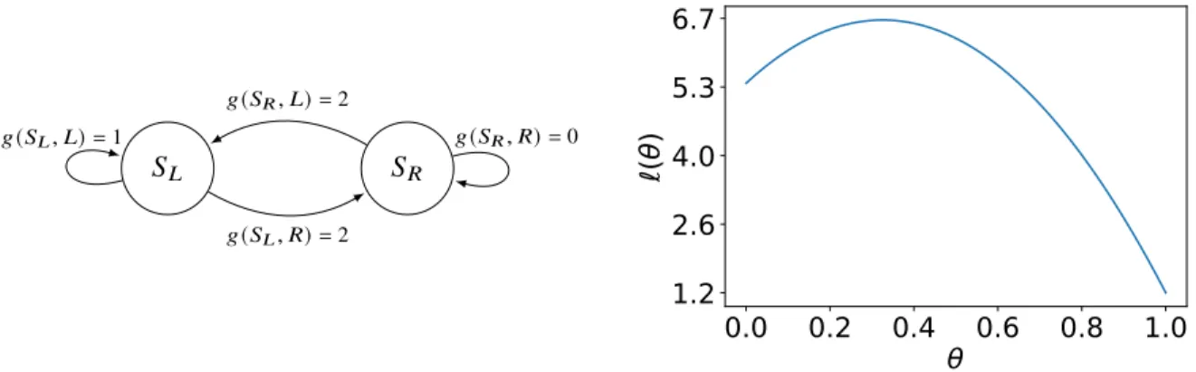
3.1 Policy gradient fails with the constrained policy class for a simple deterministic MDP. (a) Two state, two action MDP where the optimal policy, 𝜋∗ plays right in both states. (b) For the constrained policy class, 𝜋_𝜃(𝑅|𝑆_𝐿) = 𝜋_𝜃(𝑅|𝑆_𝑅) = 𝜃 ∈

[0,1], policy gradient objective is non-convex with two local minima. For (b), we took𝛾 =0.8and𝜌 = [0.6,0.4]. We remark that this example is not cherry picked. For any𝛾 > 1/2and different initial distributions 𝜌which put non-zero weight on both states,ℓ(𝜃)has two local minima at𝜃 =0and𝜃 =1. . . 60

(11)

Acknowledgements

I would like to extend my heartfelt gratitude to my advisor, Daniel Russo for sharing his excit-ing research ideas, constant encouragement and his willexcit-ingness to help at any time. He has taught me to identify and work on the most impactful ideas, unblocked me when I was stuck, been kind when I made errors and has always insisted on simple but clear writing which has often helped me clarify my own thinking. I am incredibly lucky to have had the opportunity to work closely with him. I would also like to thank Garud Iyengar for his mentorship throughout my time at Columbia. He has always supported and guided me on acedemic and non-academic issues, recommended me for internships as well as pointed me toward exciting courses and research projects. While we have never published a paper together, I have truly enjoyed all of our research discussions on a couple of projects and one day we will definitely publish a paper together.

I would also like to thank Shipra Agrawal, Christian Kroer and Krzysztof Choromanski for serving on my thesis committee. I really enjoyed working closely with Shipra on a joint project with Amazon and taking her graduate class on Reinforcement learning. I interacted with Krzysztof for the first time at AISTATS, 2017. I thank him for fruitful discussions on reseach ideas and hope to pursue research together in the future sometime. I also owe a great deal to Profs. John Cunningham and David Blei for teaching excellent graduate level courses on machine learning and including me in their weekely group meethings which got me excited about research in statstical machine learning. John and I have also co-authored two papers which were led by Francois Fagan, and are not a part of this thesis. I learnt a lot from this colloboration and research experience.

(12)

ticuarly patient with me, specially during my on-going health issues (thanks to Garud, Vineet and Jay). Along with that, I want to thank my physios, Dr. Courtney Burdowski and Dr. Lea Noonan for helping me recover which allowed me to complete this work. My fellow students in IEOR have all been very helpful and supportive. A special thanks to Itai Feigenbaum and Praveen for their words of encouragement during initial years of my PhD. I would also like to thank my undergrad-uate professors, Nomesh Bolia and Kiran Seth at IIT Delhi as well as Sandeep Juneja at TIFR, for sparking my interest in scientific research. I stayed at International House, NYC from 2014-17 and met some of the most fun people who showered me with kindness and affection. Without naming everyone, I wish to thank them all, Emad Khan and Ms Lorraine Pirro in particular.

I credit this thesis, and whatever little I have accomplished in life to my parents, people name above and everyone else who helped me so far. The numerous errors, mistakes, and failures are all attributable to me and I’ll hold onto them.

(13)

(14)

Chapter 1: Introduction

Reinforcement learning (RL) is a computational approach to automating sequential decision making where an agent learns by trial-and-error interactions with a complex, uncertain environ-ment [1]. It uses the framework of Markov decision processes to define this interaction in terms of states of the environment, actions and reward signals. The agent’s goal is to learn a decision rule (actions to take in a particular state) to maximize long run sum of the reward signal; as the action taken in the present state may not only affect the immediate reward but also change the next state. In the past decade, RL has attracted rapidly increasing interest in the machine learning and artificial intelligence communities where a primary goal is to come up with fully autonomous agents that are interactive and can continuously learn from past experiences.

With tremendous success already demonstrated on game environments like Alpha Go [2], RL algorithms offer great promise for applications to even more complex domains, for example in autonomous driving [3], robotics [4] and even drug discovery [5]. There is tremendous potential, as modeling the environments (to even reasonable approximations) in many modern applications is extremely challenging. Although researchers have devoted a lot of engineering effort to deploy RL methods at scale, many state-of-the-art RL techniques still seemmysterious– with limited the-oretical guarantees on their behavior in practice. This poses a significant challenge in convincing practitioners to use these for real world tasks. The motivation of this thesis is to understand theo-retical underpinnings of some of the key ideas in RL using tools from optimization theory. Doing this can help spur progress in principled approaches to algorithm design to tackle some key chal-lenges, for example in statistical efficiency and robustness, in applications where collecting data is difficult and expensive.

We broadly focus on two different classes of RL techniques, namely,Temporal difference learn-ingand policy gradient methods, both of which are widely adopted by practitioners and popular

(15)

among RL researchers. I considered a larger introductory chapter, but felt that it would be too repetitive in terms of context to be useful. Each chapter in this thesis is self-contained with an introduction to the problem, its motivation in context of the literature and our contribution. There-fore, we just give a brief summary of the main results below. The rest of this thesis is organized as follows.

• In Chapter 2, we consider the Temporal difference learning (TD) algorithm, which is a sim-ple iterative method used to estimate the value function corresponding to a given policy in a Markov decision process. Although widely used in reinforcement learning, theoretical analysis of TD has proved challenging and few guarantees on its statistical efficiency are available. We provide asimple and explicit finite time analysisof temporal difference learn-ing with linear function approximation. Even though TD updates arenotstochastic gradient updates with respect to any fixed loss function, our analysis uncovers key insights which en-able us to analyze TD mirroring standard techniques used for analyzing stochastic gradient descent algorithms. We also show how all of our convergence results extend seamlessly to the study of TD learning with eligibility traces, known as TD(𝜆), and to Q-learning for a class of high-dimensional optimal stopping problems.

• In Chapter 3, we consider policy gradients methods, which directly search for an optimal policy by performing stochastic gradient descent over a parameterized class of polices. Re-cently, these approaches have shown tremendous success with deep neural networks and Monte Carlo approximations to the true gradient. Unfortunately, even for simple control problems solvable by classical techniques, policy gradient algorithms face non-convex opti-mization problems and are widely understood to converge only to a local minima, assuming adequate smoothness properties. We present a simple and general understanding of global convergence properties of policy gradient methods. We focus on studying the optimization landscape and identify structural properties which guarantee despite non-convexity, any sta-tionary point of the policy gradient objective is globally optimal. We then identify conditions

(16)

mization methods, this gradient dominance conditions guarantees fast convergence rates to globally optimal solutions for non-convex objectives. Our results apply to several classic dynamic programming problems including finite MDPs, linear quadratic control, optimal stopping and finite horizon inventory control, which provide an important benchmark for studying theoretical properties of model free reinforcement learning algorithms.

• In Chapter 4, we extend our analysis of policy gradient methods for finite MDPs. We take a different perspective than that of Chapter 3, where we view this (and other problems) as an instance of smooth non-linear optimization and using gradient dominance, show sub-linear convergence with small stepsizes. Our insights in this chapter show how for tabular MDPs, different policy gradient algorithms with appropriately large step-sizes are in fact equivalent to a soft-policy iteration update and therefore enjoy linear convergence guarantees. Our analysis covers popular methods like projected policy gradient, Frank-Wolfe, mirror descent and natural policy gradient methods which are widely used in practice.

(17)

Chapter 2: A Finite Time Analysis of Temporal Difference Learning With

Linear Function Approximation

Originally proposed by [6], temporal difference learning (TD) is one of the most widely used reinforcement learning algorithms and a foundational idea on which more complex methods are built. The algorithm operates on a stream of data generated by applying some policy to a poorly understood Markov decision process. The goal is to learn an approximate value function, which can then be used to track the net present value of future rewards as a function of the system’s evolving state. TD maintains a parametric approximation to the value function, making a simple incremental update to the estimated parameter vector each time a state transition occurs.

While easy to implement, theoretical analysis of TD is subtle. Reinforcement learning re-searchers in the 1990s gathered both limited convergence guarantees [7] and examples of diver-gence [8]. Many issues were then clarified in the work of [9], which establishes precise conditions for the asymptotic convergence of TD with linear function approximation and gives examples of divergent behavior when key conditions are violated. With guarantees of asymptotic convergence in place, a natural next step is to understand the algorithm’s statistical efficiency. How much data is required to guarantee a given level of accuracy? Can one give uniform bounds on this, or could data requirements explode depending on the problem instance? Twenty years after the work of [9], such questions remain largely unsettled.

2.1 Contributions

This chapter develops asimple and explicit non-asymptotic analysis of TD with linear function approximation. The resulting guarantees provide assurances of robustness. They explicitly bound the worst-case dependence on problem features like the discount factor, the conditioning of the

(18)

feature covariance matrix, and the mixing time of the underlying Markov chain. Our analysis reveals rigorous connections between TD and stochastic gradient descent algorithms, provides a template for finite time analysis of incremental algorithms with Markovian noise, and applies without modification to analyzing a class of high-dimensional optimal stopping problems. We elaborate on these contributions below.

• Links with gradient descent: Despite a cosmetic connection to stochastic gradient descent (SGD), incremental updates of TD are not (stochastic) gradient steps with respect to any fixed loss function. It is therefore difficult to show that it makes consistent, quantifiable, progress toward its asymptotic limit point. Nevertheless, Section 2.7 shows that expected TD updates obey crucial properties mirroring those of gradient descent on a particular quadratic loss function. In a model where the observations are corrupted by i.i.d. noise, these gradient-like properties of TD allow us to give state-of-the-art convergence bounds by essentially mir-roring standard analyses of SGD. This approach may be of broader interest as SGD analyses are commonly taught in machine learning courses and serve as a launching point for a much broader literature on first-order optimization. Rigorous connections with the optimization literature can facilitate research on principled improvements to TD.

• Non-asymptotic treatment with Markovian noise: TD is usually applied online to a single Markovian data stream. However, to our knowledge, there has been no successful1 non-asymptotic analysis in the setting with Markovian observation noise. Instead, many papers have studied such algorithms under the simpler i.i.d. noise model mentioned earlier [12, 13, 14, 15, 16, 17]. One reason is that the dependent nature of the data introduces a substantial technical challenge: the algorithm’s updates are not only noisy, but can be severely biased. We use information theoretic techniques to control the magnitude of bias, yielding bounds that are essentially scaled by a factor of the mixing time of the underlying Markov process relative to those attained for the i.i.d. model. Our analysis in this setting applies only to a 1_{This was previously attempted by [10], but critical errors were shown by [11].}

(19)

variant of TD that projects the iterates onto a norm ball. This projection step imposes a uni-form bound on the noise of TD updates, which is needed for tractability. For similar reasons, projection operators are widely used throughout the stochastic approximation literature [18, Section 2].

• An extendable approach: Much of the paper focuses on analyzing the most basic tempo-ral difference learning algorithm, known as TD(0). We also extend this analysis to other algorithms. First, we establish convergence bounds for temporal difference learning with el-igibility traces, known as TD(𝜆). This is known to often outperform TD(0) [19], but a finite time analysis is more involved. Our analysis also applies without modification to Q-learning for a class of high-dimensional optimal stopping problems. Such problems have been widely studied due to applications in the pricing of financial derivatives [20, 21, 22, 23, 24]. For our purposes, this example illustrates more clearly the link between value prediction and decision-making. It also shows our techniques extend seamlessly to analyzing an instance of linear stochastic approximation. To our knowledge, no prior work has provided non-asymptotic guarantees for either TD(𝜆) or Q-learning with function approximation.

2.2 Related Literature

Non-asymptotic analysis of TD(0): There has been very little non-asymptotic analysis of TD(0). To our knowledge, [10] provided the first finite time analysis. However, several serious errors in their proofs were pointed out by [11]. A very recent work by [25] studies TD(0) with linear function approximation in an i.i.d. observation model, which assumes sequential observations used by the algorithm are drawn independently from their steady-state distribution. They focus on analysis with problem independent step-sizes of the form1/𝑇𝜎 for a fixed𝜎 ∈ (0,1)and establish that mean-squared error converges at a rate2 of 𝑂(1/𝑇𝜎). Unfortunately, while the analysis is technically non-asymptotic, the constant factors in the bound display a complex dependence on 2_{In personal communication, the authors have told us their analysis also yields a}_𝑂₍₁_/_𝑇₎_{rate of convergence for}

(20)

the problem instance and scale with some unusual quantities which can be very large in cases of practical interest.

Another interesting paper by [17] studies linear stochastic approximation algorithms under i.i.d. noise, including TD(0), with constant step-sizes and iterate averaging. This approach dates back to the works of [26, 27] and [28], which shows that the iterates of a constant step-size linear stochastic approximation algorithm form an ergodic Markov chain and,in the case of i.i.d. observation noise, their expectation in steady-state is equal to the true solution of the linear system. By a central limit theorem for ergodic sequences, the average iterate converges to the true solution, with mean-squared error decaying at rate 𝑂(1/𝑇). [29] give a sophisticated non-asymptotic analysis of the least-mean-squares algorithm with constant step-size and iterate-averaging. [17] aim to understand whether such guarantees extend to linear stochastic approximation algorithms more broadly. In the process, their work provides𝑂(1/𝑇)bounds for iterate-averaged TD(0) with constant step-size. A remarkable feature of their approach is that the choice of step-size is independent of the condition-ing of the features (although the bounds themselves do degrade if features become ill-conditioned). It is worth noting that these results rely critically on the assumption that noise is i.i.d. This is not due to any shortcoming in the techniques of [29] and [17]. Instead, under non-i.i.d. noise and a linear stochastic approximation algorithm applied with any constant step-size, the averaged-iterate might converge to the wrong limit as shown in a simple example by [28].

The recent works of [25] and [17] give bounds for TD(0) only under i.i.d. observation noise. Therefore their results are most comparable to what is presented in Section 2.8. For the i.i.d. noise model, the main argument in favor of our approach is that it allows for extremely simple proofs, interpretable constant terms, and illuminating connections with SGD. Moreover, it is worth em-phasizing that our approach gracefully extends to more complex settings, including more realistic models with Markovian noise, the analysis of TD with eligibility traces, and the analysis of Q-learning for optimal stopping problems as shown in Sections 2.9, 2.10 and 2.11.

While not directly comparable to our results, we point the readers to the excellent work of [30]. To facilitate theoretical analysis, they consider a slightly modified version of the TD(𝜆) algorithm.

(21)

The authors provide a finite time analysis for this algorithm in an adversarial model where the goal is to predict the discounted sum of future rewards from each state. Performance is measured relative to the best fixed linear predictor in hindsight. The analysis is creative, but results depend on a several unknown constants and on the specific sequence of states and rewards on which the algorithm is applied. [30] also apply their techniques to study value function approximation in a Markov decision process. In that case, the bounds are much weaker than what is established here. Their bound scales with the size of the state space, which is enormous in most practical problems – and applies only to TD(1), a somewhat degenerate special case of TD(𝜆) in which it is equivalent to Monte Carlo policy evaluation [19].

Asymptotic analysis of stochastic approximation: There is a well developed theory around asymptotic analysis of stochastic approximation, a field that studies noisy recursive algorithms like TD [31, 32, 33]. Most asymptotic convergence proofs in reinforcement learning use a technique known as the ODE method [34]. Under some technical conditions and appropriate decaying step-sizes, this method ensures the almost-sure convergence of stochastic approximation algorithms to the invariant set of a certain ‘mean’ differential equation. The technique greatly simplifies asymp-totic convergence arguments, since it completely circumvents issues with noise in the system and issues of step-size selection. But this also makes it a somewhat coarse tool, unable to generate in-sight into an algorithm’s sensitivity to noise, ill-conditioning, or step-size choices. A more refined set of techniques begin to address these issues. Under fairly broad conditions, a central limit the-orem for stochastic approximation algorithms characterizes their limiting variance. Such a central limit theorem has been specifically provided for TD by [35] and [36].

In addition to such asymptotic techniques, the modern literature on first-order stochastic op-timization also focuses heavily on non-asymptotic analysis [37, 38, 39]. One reason is that such asymptotic analysis necessarily focuses on a regime where step-sizes are negligibly small relative to problem features and the iterates have already converged to a small neighborhood of the opti-mum. However, the use of a first-order method in the first place signals that a practitioner is mostly

(22)

interested in cheaply reaching a reasonably accurate solution, rather than the rate of convergence in the neighborhood of the optimum. In practice, it is common to use constant step-sizes, so iter-ates never truly converge to the optimum. A non-asymptotic analysis requires grappling with the algorithm’s behavior in practically relevant regimes where step-sizes are still relatively large and iterates are not yet close to the true solution.

Analysis of related algorithms: A number of papers analyze algorithms related to and inspired by the classic TD algorithm. First, among others, [40, 41, 42, 43, 44] and [45] analyze least-squares temporal difference learning (LSTD). [46] study the related least-least-squares policy iteration algorithm. The asymptotic limit point of TD is a minimizer of a certain population loss, known as the mean-squared projected Bellman error. LSTD solves a least-squares problem, essentially computing the exact minimizer of this loss on the empirical data. It is easy to derive a central limit theorem for LSTD. Finite time bounds follow from establishing uniform convergence rates of the empirical loss to the population loss. Unfortunately, such techniques appear to be quite distinct from those needed to understand the online TD algorithms studied in this paper. Online TD has seen much wider use due to significant computational advantages [19].

Gradient TD methods are another related class of algorithms. These were derived by [13, 12] to address the issue that TD can diverge in so-called “off-policy” settings, where data is collected from a policy different from the one for which we want to estimate the value function. Unlike the classic TD(0) algorithm, gradient TD methods are designed to mimic gradient descent with respect to the mean squared projected Bellman error. [13, 12] propose asymptotically conver-gent two-time scale stochastic approximation schemes based on this and more recently [16] give a finite time analysis of two time scale stochastic approximation algorithms, including several vari-ants of gradient TD algorithms. Alternatively, [47] and [14] propose to reformulate the original gradient TD optimization as a primal-dual saddle point problem and leverage convergence analy-sis form that literature to give a non-asymptotic analyanaly-sis. This work was later revisited by [15], who established a faster rate of convergence. The works of [16, 14] and [15] all consider only

(23)

i.i.d. observation noise. One interesting open question is whether our techniques for treating the Markovian observation model will also apply to these analyses. Finally, it is worth highlighting that, to the best of our knowledge, substantial new techniques are needed to analyze the widely used TD(0), TD(𝜆) and the Q-learning studied in this paper. Unlike gradient TD methods, they do not mimic noisy gradient steps with respect to any fixed objective3.

2.3 Problem formulation

Markov reward process. We consider the problem of evaluating the value function 𝑉_𝜇 of a given policy 𝜇in a Markov decision process (MDP). We work in theon policysetting, where data is generated by applying the policy 𝜇in the MDP. Because the policy 𝜇is applied automatically to select actions, such problems are most naturally formulated as value function estimation in a Markov reward process (MRP). A MRP4 comprises of (S,P,R, 𝛾) [19] where S is the set of finite states,Pis the Markovian transition kernel,Ris a reward function, and𝛾 <1is the discount factor. For a discrete state-spaceS, P (𝑠0|𝑠) specifies the probability of transitioning from a state 𝑠 to another state 𝑠0. The reward functionR (𝑠, 𝑠0) associates a reward with each state transition. We denote byR (𝑠) =Í

𝑠0∈SP (𝑠 0_|

𝑠)R (𝑠, 𝑠0)the expected instantaneous reward generated from an initial state𝑠.

The value function associated with this MRP,𝑉𝜇, specifies the expected cumulative discounted

future reward as a function of the state of the system. In particular,

𝑉_𝜇(𝑠) =_E " _∞ Õ 𝑡=0 𝛾𝑡R (𝑠_𝑡) | 𝑠₀=𝑠 # ,

where the expectation is over sequences of states generated according to the transition kernel P. This value function obeys the Bellman equation𝑇_𝜇𝑉_𝜇 =𝑉_𝜇, where the Bellman operator𝑇_𝜇 asso-3_{This can be formally verified for TD(0) with linear function approximation. If the TD step were a gradient with}

respect to a fixed objective, differentiating it should give the Hessian and hence a symmetric matrix. Instead, the matrix one attains is typically not a symmetric one.

(24)

ciates a value function𝑉 :S →_Rwith another value function𝑇_𝜇𝑉 satisfying

(𝑇𝜇𝑉) (𝑠)=R (𝑠) +𝛾

Õ

𝑠0∈S

P (𝑠0|𝑠)𝑉(𝑠0) ∀ 𝑠∈ S.

We assume rewards are bounded uniformly such that

|R (𝑠, 𝑠0) | ≤𝑟_max ∀ 𝑠, 𝑠0 ∈ S.

Under this assumption, value functions are assured to exist and are the unique solution to Bellman’s equation [48]. We also assume that the Markov reward process induced by following the policy 𝜇 is ergodic with a unique stationary distribution 𝜋. For any two states𝑠, 𝑠0: 𝜋(𝑠0) =lim_𝑡_→∞_P(𝑠_𝑡 = 𝑠0|𝑠₀ =𝑠).

Following common references [48, 49, 50], we will simplify the presentation by assuming the state space S is a finite set of size 𝑛 = |S |. Working with a finite state space allows for the use of compact matrix notation, which is the convention in work on linear value function approximation. It also avoids measure theoretic notation for conditional probability distributions. Our proofs extend in an obvious way to problems with countably infinite state-spaces, as long the uniform ergodicity condition stated in Section 2.9, Assumption 1, continues to hold. For problems with general state-space, even the core results in dynamic programming hold only under suitable technical conditions [51].

Value function approximation. Given a fixed policy𝜇, the problem is to efficiently estimate the corresponding value function𝑉𝜇 using only the observed rewards and state transitions.

Unfortu-nately, due to the curse of dimensionality, most modern applications have intractably large state spaces, rendering exact value function learning hopeless. Instead, researchers resort to parametric approximations of the value function, for example by using a linear function approximator [19] or a non-linear function approximation such as a neural network [52]. In this work, we consider a

(25)

linear function approximation architecture where the true value-to-go𝑉_𝜇(𝑠) is approximated as

𝑉𝜇(𝑠) ≈𝑉𝜃(𝑠) =𝜙(𝑠) >

𝜃 ,

where𝜙(𝑠) ∈_R𝑑is a fixed feature vector for state𝑠and𝜃 ∈_R𝑑is a parameter vector that is shared across states. When the state space is the finite set S = {𝑠₁, . . . , 𝑠_𝑛}, 𝑉_𝜃 ∈ _R𝑛 can be expressed compactly as 𝑉_𝜃 =           𝜙(𝑠₁)> . . . 𝜙(𝑠_𝑛)>           𝜃 =           𝜙₁(𝑠₁) 𝜙_𝑘(𝑠₁) 𝜙_𝑑(𝑠₁) . . . . . . . . . 𝜙₁(𝑠_𝑛) 𝜙_𝑘(𝑠_𝑛) 𝜙_𝑑(𝑠_𝑛)           𝜃 = Φ𝜃 , whereΦ∈ _R𝑛×𝑑

and𝜃 ∈_R𝑑. We assume throughout that the𝑑 features vectors{𝜙_𝑘}𝑑

𝑘=1, forming

the columns ofΦare linearly independent.

Norms in value function and parameter space. For a symmetric positive definite matrix 𝐴, define the inner product h𝑥 , 𝑦i_𝐴 = 𝑥>𝐴 𝑦and the associated norm k𝑥k_𝐴 =

√

𝑥>𝐴𝑥 .If 𝐴is positive

semi-definite rather than positive definite thenk·k𝐴is called a semi-norm. Let𝐷 =diag(𝜋(𝑠1), . . . , 𝜋(𝑠𝑛)) ∈

R𝑛×𝑛denote the diagonal matrix whose elements are given by the entries of the stationary distribu-tion𝜋(·). Then, for two value functions𝑉 and𝑉0,

k𝑉 −𝑉0k_𝐷 =

s Õ

𝑠∈S

𝜋(𝑠) (𝑉(𝑠) −𝑉0(𝑠))2,

measures the mean-square difference between the value predictions under𝑉and𝑉0, in steady-state. This suggests a natural norm on the space of parameter vectors. In particular, for any𝜃 , 𝜃0 ∈_R𝑑,

k𝑉𝜃−𝑉𝜃0k𝐷 =

s Õ

𝑠∈S

(26)

where

Σ := Φ>𝐷Φ =

Õ

𝑠∈S

𝜋(𝑠)𝜙(𝑠)𝜙(𝑠)> is the steady-state feature covariance matrix.

Feature regularity. We assume that feature vectors are uniformly bounded, that issup𝑠∈S k𝜙(𝑠) k2 < ∞. For notational convenience, we assume features are normalized so that k𝜙(𝑠) k₂ ≤ 1 for all 𝑠 ∈ S. This is without loss of generality because the TD algorithm is invariant to feature re-scaling. Precisely, TD applied with feature mapping 𝜙(·) and initial parameter 𝜃₀ produces an identical sequence of value functions to the TD algorithm with feature mapping𝜙˜(·) = 𝑘 𝜙(·)and initial parameter𝜃˜₀=𝜃₀/𝑘, for any scalar𝑘 > 0. Note that all our results bound the mean-squared gap between value predictions. We also assume that any entirely redundant or irrelevant features have been removed, so Σ has full rank. Let 𝜔 > 0 be the minimum eigenvalue of Σ. From our bound on the feature vectors, the maximum eigenvalue ofΣis less than1, so1/𝜔bounds the condi-tion number of the feature covariance matrix5. The following lemma is an immediate consequence of our assumptions.

Lemma 1(Norm equivalence). For all𝜃 ∈_R𝑑,

√

𝜔k𝜃k₂≤ k𝑉𝜃k𝐷 ≤ k𝜃k2.

One typical style of result in the study of strongly convex optimization gives fast rates of convergence in terms of the number of iterations𝑇. But these bounds degrade when 𝜔 is very small and generally require apriori knowledge of some good lower bound on𝜔. We give some results in that style, but also give results in the style of [53], where bounds and stepsizes have no dependence on𝜔.

2.4 Temporal difference learning

We consider the classic temporal difference learning algorithm [6]. The algorithm starts with an initial parameter estimate𝜃₀and at every time step 𝑡, it observes one data tuple𝑂𝑡 = (𝑠𝑡, 𝑟𝑡 =

5_Let_𝜆

max(𝐴) = max_k𝑥k₂=1𝑥

>

𝐴𝑥 denote the maximum eigenvalue of a symmetric positive-semidefinite matrix.

Since this is a convex function,𝜆_max(Σ) ≤Í

𝑠∈S𝜋(𝑠)𝜆max(𝜙(𝑠)𝜙(𝑠)

>_{) ≤}Í

(27)

R (𝑠_𝑡, 𝑠0

𝑡), 𝑠 0

𝑡)consisting of the current state, the current reward and the next state reached by playing

policy 𝜇in the current state. This tuple is used to define a loss function, which is taken to be the squared sample Bellman error. The algorithm then proceeds to compute the next iterate 𝜃_𝑡₊₁ by taking a gradient-like update. Some of our bounds guarantee accuracy of the average iterate, denoted by𝜃¯𝑡 =𝑡

−1Í𝑡−1

𝑖=0𝜃𝑖. The version of TD presented in Algorithm 1 below also makes online

updates to the averaged iterate.

TD is not a true stochastic gradient method with respect to any fixed loss function, which makes its analysis challenging. The TD update can be written as𝑔_𝑡(𝜃) = (𝑦_𝑡 −𝑉_𝜃(𝑠_𝑡)) 𝑑

𝑑𝜃𝑉𝜃(𝑠𝑡),

where 𝑦_𝑡 = 𝑟_𝑡 +𝛾𝑉_𝜃(𝑠0

𝑡) is a sample based estimate of the Bellman update to𝑉𝜃𝑡. Then𝑔𝑡(𝜃𝑡) = − 𝜕 𝜕 𝜃 1 2(𝑦𝑡 −𝑉𝜃(𝑠𝑡)) 2

𝜃=𝜃𝑡 can be interpreted as the negative gradient of a certain squared loss

func-tion, but this calculation treats the target 𝑦𝑡 as fixed and ignores its implicit dependence on 𝜃𝑡.

To emphasize the contrast with stochastic gradient methods, [19] refer to TD as a semi-gradient method. Accordingly, we will refer to𝑔_𝑡(·)asnegative semi-gradientthroughout the paper.

We present in Algorithm 1 the simplest variant of TD, which is known as TD(0). It is also worth highlighting that here we study online temporal difference learning, which makes incremental semi-gradient updates to the parameter estimate based on the most recent data observations only. Such algorithms are widely used in practice, but harder to analyze than so-called batch TD methods like the LSTD algorithm of [54].

Algorithm 1:TD(0) with linear function approximation Input :initial guess𝜃₀, step-size sequence{𝛼_𝑡}_𝑡_∈

N. Initialize: 𝜃¯₀←𝜃₀. for𝑡 =0,1, . . .do Observe tuple:𝑂_𝑡 = (𝑠_𝑡, 𝑟_𝑡 =R (𝑠_𝑡, 𝑠0 𝑡), 𝑠 0 𝑡) Define target: 𝑦𝑡 =R (𝑠𝑡, 𝑠 0 𝑡) +𝛾𝑉𝜃𝑡(𝑠 0

𝑡) /* sample Bellman operator */

Loss function: 1₂(𝑦𝑡−𝑉𝜃(𝑠𝑡))2 /* sample Bellman error squared */

Compute negative semi-gradient: 𝑔𝑡(𝜃𝑡) =− 𝜕 𝜕 𝜃 1 2(𝑦𝑡−𝑉𝜃(𝑠𝑡))2 𝜃=𝜃𝑡

Take a semi-gradient step: 𝜃_𝑡₊₁=𝜃_𝑡 +𝛼_𝑡𝑔_𝑡(𝜃_𝑡) /* 𝛼_𝑡:step-size */ Update averaged iterate: 𝜃¯_𝑡₊₁← 𝑡

𝑡+1 _¯ 𝜃_𝑡+ 1 𝑡+1 𝜃_𝑡 /* 𝜃¯_𝑡₊₁= 1 𝑡+1 Í𝑡 ℓ=0𝜃ℓ */ end

(28)

the current parameter. As a general function of 𝜃 and the tuple 𝑂_𝑡 = (𝑠_𝑡, 𝑟_𝑡, 𝑠0

𝑡), the negative

semi-gradient can be written as

𝑔_𝑡(𝜃) = 𝑟_𝑡+𝛾 𝜙(𝑠0 𝑡) > 𝜃−𝜙(𝑠_𝑡)>𝜃 𝜙(𝑠_𝑡). (2.1)

The long-run dynamics of TD are closely linked to the expected negative semi-gradient step when the tuple𝑂_𝑡 =(𝑠_𝑡, 𝑟_𝑡, 𝑠0

𝑡) follows itssteady-statebehavior:

¯ 𝑔(𝜃):=

Õ

𝑠,𝑠0∈S

𝜋(𝑠)P (𝑠0|𝑠) R (𝑠, 𝑠0) +𝛾 𝜙(𝑠0)>𝜃−𝜙(𝑠)>𝜃𝜙(𝑠) ∀𝜃 ∈_R𝑑.

This can be rewritten more compactly in several useful ways. One such way is,

¯

𝑔(𝜃) =_E[𝜙𝑟] +_E𝜙(𝛾 𝜙0−𝜙)>𝜃 , (2.2)

where 𝜙 = 𝜙(𝑠) is the feature vector of a random initial state 𝑠 ∼ 𝜋, 𝜙0 = 𝜙(𝑠0) is the feature vector of a random next state drawn according to𝑠0∼ P (· | 𝑠), and𝑟 =R (𝑠, 𝑠0). In addition, since

Í

𝑠0∈SP (𝑠 0_|

𝑠) (R (𝑠, 𝑠0) +𝛾 𝜙(𝑠0)>𝜃) = (𝑇𝜇Φ𝜃) (𝑠), we can recognize that

¯

𝑔(𝜃) = Φ>𝐷(𝑇_𝜇Φ𝜃−Φ𝜃). (2.3)

See [9] for a derivation of this fact.

2.5 Asymptotic convergence of temporal difference learning

The main challenge in analyzing TD is that the semi-gradient steps𝑔_𝑡(𝜃)are not true stochastic gradients with respect to any fixed objective. The semi-gradient step taken at time𝑡pulls the value prediction𝑉_𝜃𝑡

+1(𝑠𝑡)closer to𝑦𝑡, but𝑦𝑡itself depends on𝑉𝜃𝑡. So does this circular process converge?

The key insight of [9] was to interpret this as a stochastic approximation scheme for solving a fixed point equation known as the projected Bellman equation. Contraction properties together

(29)

with general results from stochastic approximation theory can then be used to show convergence. Should TD converge at all, it should be to a stationary point. Because the feature covariance matrix Σis full rank there is a unique6 vector𝜃∗ with 𝑔¯(𝜃∗) = 0. We briefly review results that offer insight into𝜃∗and proofs of the asymptotic convergence of TD.

Understanding the TD limit point. Tsitsiklis and Van Roy [9] give an interesting characteriza-tion of the limit point𝜃∗. They show it is the unique solution to theprojectedBellman equation

Φ𝜃= Π_𝐷𝑇_𝜇Φ𝜃 , (2.4)

whereΠ𝐷(·)is the projection operator onto the subspace{Φ𝑥 |𝑥 ∈R 𝑑

}spanned by these features in the inner product h·,·i𝐷. To see why this is the case, note that by using𝑔¯(𝜃

∗₎ ₌ ₀ _{along with}

Equation (2.3),

0=𝑥>𝑔¯(𝜃∗) =hΦ𝑥 , 𝑇_𝜇Φ𝜃∗−Φ𝜃∗i_𝐷 ∀𝑥 ∈_R𝑑.

That is, the Bellman error at𝜃∗, given by(𝑇_𝜇Φ𝜃∗−Φ𝜃∗), is orthogonal to the space spanned by the features in the inner product h·,·i_𝐷. By definition, this meansΠ_𝐷 𝑇_𝜇Φ𝜃∗−Φ𝜃∗ = 0and hence 𝜃∗ must satisfy the projected Bellman equation.

The following lemma shows the projected Bellman operator,Π𝐷𝑇𝜇(·)is a contraction, and so in

principle, one could converge to the approximate value functionΦ𝜃∗by repeatedly applying it. TD appears to serve as a simple stochastic approximation scheme for solving the projected-Bellman fixed point equation.

Lemma 2. [Tsitsiklis and Van Roy [9]] Π𝐷𝑇𝜇(·) is a contraction with respect to k · k𝐷 with

modulus𝛾, that is,

Π𝐷𝑇𝜇𝑉𝜃−Π𝐷𝑇𝜇𝑉𝜃0 𝐷 ≤ 𝛾k𝑉_𝜃 −𝑉_𝜃0k 𝐷 ∀𝜃 , 𝜃 0 _∈ R𝑑.

(30)

argument shows 𝑉_𝜃∗ −𝑉_𝜇 𝐷 ≤ 1 p 1−𝛾2 Π𝐷𝑉𝜇 −𝑉𝜇 𝐷 . (2.5)

See Chapter 6 of [48] for a proof. The left hand side of Equation (2.5) measures the root-mean-squared deviation between the value predictions of the limiting TD value function and the true value function. On the right hand side, the projected value functionΠ𝐷𝑉𝜇 minimizes

root-mean-squared prediction errors among all value functions in the span ofΦ. If𝑉_𝜇 actually falls within the span of the features, there is no approximation error at all and TD converges to the true value function.

Asymptotic convergence via the ODE method. Like many analyses in reinforcement learning, the convergence proof of [9] appeals to a powerful technique from the stochastic approximation literature known as the “ODE method”. Under appropriate conditions, and assuming a decaying step-size sequence satisfying the Robbins-Monro conditions, this method establishes the asymp-totic convergence of the stochastic recursion 𝜃𝑡+1 = 𝜃𝑡 +𝛼𝑡𝑔𝑡(𝜃𝑡) as a consequence of the global

asymptotic stability of the deterministic ODE:𝜃¤_𝑡 =𝑔¯(𝜃_𝑡). The critical step in the proof of [9] is to use the contraction properties of the Bellman operator to establish this ODE is globally asymptot-ically stable with the equilibrium point𝜃∗.

The ODE method vastly simplifies convergence proofs. First, because the continuous dynamics can be easier to analyze than discretized ones, and more importantly, because it avoids dealing with stochastic noise in the problem. At the same time, by side-stepping these issues, the method offers little insight into the critical effect of step-size sequences, problem conditioning, and mixing time issues on algorithm performance.

2.6 Outline of analysis

The remainder of this chapter focuses on a finite time analysis of TD. Broadly, we establish two types of finite time bounds onEk𝑉_¯

𝜃𝑇 −

𝑉_𝜃∗k2 𝐷

, which measures the mean-squared gap between the value predictions under the averaged-iterate𝜃¯𝑇 and under the TD limit point𝜃

(31)

bounds that depend on the condition number of the feature covariance matrix. These mirror what one might expect from the literature on stochastic optimization of strongly convex functions: re-sults showing that TD with constant step-sizes converges to within a radius of𝑉_𝜃∗at an exponential

rate, and𝑂(1/𝑇)convergence rates with appropriate decaying step-sizes.

These results establish fast rates of convergence, but only if the problem is well conditioned. The choice of step-sizes is also very sensitive to problem conditioning. Work on robust stochastic approximation [53] argues instead for the use of comparatively large step-sizes together with iterate averaging7. Following the spirit of this work, we also give explicit bounds on Ek𝑉_¯

𝜃𝑇 −𝑉𝜃∗k 2 𝐷 with a slower 𝑂(1/ √

𝑇) convergence rates, but importantly both the bounds and step-sizes are completely independent of problem conditioning.

Our approach is to start by developing insights from simple, stylized settings, and then incre-mentally extend the analysis to more complex settings. The analysis is outlined below.

Noiseless case: Drawing inspiration from the ODE method discussed above, we start by analyz-ing the Euler discretization of the ODE 𝜃¤_𝑡 = 𝑔¯(𝜃_𝑡), which is the deterministic recursion 𝜃_𝑡₊₁ = 𝜃_𝑡 +𝛼𝑔¯(𝜃_𝑡). We call this method “mean-path TD”. As motivation, the section first considers a fictitious gradient descent algorithm designed to converge to the TD fixed point. We then develop striking analogues for mean-path TD of the key properties underlying the convergence of gradient descent. Easy proofs then yield two bounds mirroring those given for gradient descent.

Independent noise: Section 2.8 studies TD under an i.i.d. observation model, where the data-tuples used by TD are drawn i.i.d. from the stationary distribution. The techniques used to analyze mean-path TD(0) extend easily to this setting, and the resulting bounds mirror standard guarantees for stochastic gradient descent.

Markov noise: In Section 2.9, we analyze TD in the more realistic setting where the data is col-7_{This approach argues for using step-sizes of the order of}₁_/√_𝑡_{, where}_𝑡_{is the current iteration. These are much}

larger than the stepsizes, on the order of1/𝑡, that are suggested in the classical stochastic approximation literature.

(32)

lected from a single sample path of an ergodic Markov chain. This setting introduces signif-icant challenges due to the highly dependent nature of the data. For tractability, we assume the Markov chain satisfies a certain uniform bound on the rate at which it mixes, and study a variant of TD that uses a projection step to ensure uniform boundedness of the iterates. In this case, our results essentially scale by a factor of the mixing time relative to the i.i.d. case. Extension to TD(𝜆): In Section 2.10, we extend the analysis under the Markov noise to TD with eligibility traces, popularly known as TD(𝜆). Eligibility traces are known to often provide performance gains in practice, but theoretical analysis is more complex. Such analysis offers some insight into the subtle tradeoffs in the selection of the parameter𝜆 ∈ [0,1].

Approximate optimal stopping: A final section extends our results to a class of high dimen-sional optimal stopping problems. We analyze Q-learning with linear function approxima-tion. Building on observations of [20], we show the key properties used in our analysis of TD continue to hold for Q-learning in this setting. The convergence bounds shown in Sections 2.8 and 2.9 therefore applywithout any modification.

2.7 Analysis of mean-path TD

All practical applications of TD involve observation noise. However, a great deal of insight can be gained by investigating a natural deterministic analogue of the algorithm. Here we study the recursion

𝜃_𝑡₊₁=𝜃_𝑡+𝛼𝑔¯(𝜃_𝑡) 𝑡 ∈_N₀ ={0,1,2, . . .},

which is the Euler discretization of the ODE described in Section 2.5. We will refer to this iterative algorithm asmean-path TD. In this section, we develop key insights into the dynamics of mean-path TD that allow for a remarkably simple finite time analysis of its convergence. Later sections of the paper show how these ideas extend gracefully to analyses with observation noise.

The key to our approach is to develop properties of mean-path TD that closely mirror those of gradient descent on a particular quadratic loss function. To this end, in the next subsection, we

(33)

review a simple analysis of gradient descent. In Subsection 2.7.2, we establish key properties of mean-path TD mirroring those used to analyze this gradient descent algorithm. Finally, Subsection 2.7.3 gives convergence rates of mean-path TD, with proofs and rates mirroring those given for gradient descent except for a constant that depends on the discount factor,𝛾.

2.7.1 Gradient descent on a value function loss Consider the cost function

𝑓(𝜃) = 1 2k𝑉𝜃∗ −𝑉𝜃k 2 𝐷 = 1 2k𝜃 ∗₋ 𝜃k2 Σ,

which measures the mean-squared gap between the value predictions under 𝜃 and those under the stationary point of TD, 𝜃∗. Consider as well a hypothetical algorithm that performs gradient descent on 𝑓, iterating 𝜃_𝑡₊₁ = 𝜃_𝑡 − 𝛼∇𝑓(𝜃_𝑡) for all 𝑡 ∈ _N₀. Of course, this algorithm is not implementable, as one does not know the limit point𝜃∗of TD. However, reviewing an analysis of such an algorithm will offer great insights into our eventual analysis of TD.

To start, a standard decomposition characterizes the evolution of the error at iterate𝜃_𝑡:

k𝜃∗−𝜃_𝑡₊₁k2 2= k𝜃 ∗₋ 𝜃_𝑡k2 2+2𝛼∇𝑓(𝜃𝑡) >₍ 𝜃∗−𝜃_𝑡) +𝛼2k∇𝑓(𝜃_𝑡) k2 2.

To use this decomposition, we need two things. First, some understanding of∇𝑓(𝜃𝑡) >₍

𝜃∗ −𝜃𝑡),

capturing whether the gradient points in the direction of(𝜃∗−𝜃_𝑡). And second, we need an upper bound on the norm of the gradient k∇𝑓(𝜃_𝑡) k2

2. In this case, ∇𝑓(𝜃) = Σ(𝜃 −𝜃 ∗₎ , from which we conclude ∇𝑓(𝜃)>(𝜃∗−𝜃) =−k𝜃∗−𝜃k2 Σ =−k𝑉𝜃∗−𝑉𝜃k 2 𝐷. (2.6)

(34)

In addition, one can show8

k∇𝑓(𝜃) k₂ ≤ k𝑉_𝜃∗ −𝑉_𝜃k_𝐷. (2.7) Now, using (2.6) and (2.7), we have that for step-size𝛼=1,

k𝜃∗−𝜃_𝑡₊₁k2 2 ≤ k𝜃 ∗₋ 𝜃_𝑡k2 2− k𝑉𝜃∗−𝑉𝜃𝑡k 2 𝐷. (2.8)

The distance to𝜃∗decreases in every step, and does so more rapidly if there is a large gap between the value predictions under𝜃and𝜃∗. Combining this with Lemma 1 gives

k𝜃∗−𝜃_𝑡₊₁k2 2 ≤ (1−𝜔) k𝜃 ∗₋ 𝜃_𝑡k2 2 ≤ . . .≤ (1−𝜔) 𝑡+1 k𝜃∗−𝜃₀k2 2. (2.9)

Recall that 𝜔 denotes the minimum eigenvalue of Σ. This shows that error converges at a fast geometric rate. However the rate of convergence degrades if the minimum eigenvalue𝜔is close to zero. Such a convergence rate is therefore only meaningful if the feature covariance matrix is well conditioned.

By working in the space of value functions and performing iterate averaging, one can also give a guarantee that is independent of𝜔. Recall the notation𝜃¯_𝑇 =𝑇−1Í𝑇−1

𝑡=0 𝜃𝑡for the averaged iterate.

A simple proof from (2.8) shows

k𝑉_𝜃∗−𝑉_¯ 𝜃𝑇k 2 𝐷 ≤ 1 𝑇 𝑇−1 Õ 𝑡=0 k𝑉_𝜃∗−𝑉_𝜃𝑡k2 𝐷 ≤ k𝜃∗−𝜃₀k2 2 𝑇 . (2.10)

2.7.2 Key properties of mean-path TD

This subsection establishes analogues for mean-path TD of the key properties (2.6) and (2.7) used to analyze gradient descent. First, to characterize the semi-gradient update, our analysis

8_{This can be seen from the fact that for any vector}_𝑢_with_k_𝑢_k

2 ≤1,

(35)

builds on Lemma 7 of [9], which uses the contraction properties of the projected Bellman operator to conclude that

¯

𝑔(𝜃)>(𝜃∗−𝜃) > 0 ∀𝜃 ≠𝜃∗. (2.11) That is, the expected update of TD always forms a positive angle with (𝜃∗ − 𝜃). Though only Equation (2.11) was stated in their lemma, [9] actually reach a much stronger conclusion in their proof itself. This result, given in Lemma 3 below, establishes that the expected updates of TD point in a descent direction of k𝜃∗−𝜃k2

2, and do so more strongly when the gap between value functions

under𝜃and𝜃∗is large. We will show that this more quantitative form of (2.11) allows for elegant finite time-bounds on the performance of TD.

Note that this lemma mirrors the property in Equation (2.6), but with a smaller constant of(1−

𝛾). This reflects that expected TD must converge to𝜃∗by bootstrapping [6] and may follow a less direct path to𝜃∗ than the fictitious gradient descent method considered in the previous subsection. Recall that the limit point𝜃∗solves𝑔¯(𝜃∗)=0.

Lemma 3. For any𝜃 ∈_R𝑑,

¯

𝑔(𝜃)>(𝜃∗−𝜃) ≥ (1−𝛾) k𝑉_𝜃∗−𝑉_𝜃k2

𝐷.

Proof. We use the notation described in Equation (2.2) of Section 2.4. Consider a stationary sequence of states with random initial state 𝑠 ∼ 𝜋 and subsequent state 𝑠0, which, conditioned on𝑠, is drawn fromP (·|𝑠). Set𝜙=𝜙(𝑠),𝜙0=𝜙(𝑠0)and𝑟 =R (𝑠, 𝑠0). Define𝜉 =𝑉_𝜃∗(𝑠) −𝑉_𝜃(𝑠)=

(𝜃∗−𝜃)>𝜙and 𝜉0 =𝑉_𝜃∗(𝑠0) −𝑉_𝜃(𝑠0) = (𝜃∗ −𝜃)>𝜙0. By stationarity, 𝜉 and𝜉0are two correlated random variables with the same marginal distribution. By definition,E[𝜉2] =k𝑉_𝜃∗−𝑉_𝜃k2

𝐷 since𝑠

is drawn from𝜋.

Using the expression for𝑔¯(𝜃)in Equation (2.2),

¯

(36)

Therefore

(𝜃∗−𝜃)>𝑔¯(𝜃) =_E[𝜉(𝜉−𝛾 𝜉0)] =_E[𝜉2] −𝛾_E[𝜉0𝜉] ≥ (1−𝛾)_E[𝜉2] =(1−𝛾) k𝑉𝜃∗−𝑉𝜃k 2 𝐷.

The inequality above uses Cauchy-Schwartz inequality together with the fact that𝜉and𝜉0have the same marginal distribution to concludeE[𝜉 𝜉0] ≤

p

E[𝜉2]

p

E[(𝜉0)2] =_E[𝜉2]. Lemma 4 is the other key ingredient to our results. It upper bounds the norm of the expected negative semi-gradient, providing an analogue of Equation (2.7).

Lemma 4. k𝑔¯(𝜃) k₂ ≤ 2k𝑉_𝜃−𝑉_𝜃∗k_𝐷 ∀𝜃 ∈_R𝑑.

Proof. Beginning from (2.12) in the Proof of Lemma 3, we have

k𝑔¯(𝜃) k₂= k_E[𝜙(𝜉−𝛾 𝜉0)] k₂ ≤ q Ek𝜙k2 2 q E(𝜉−𝛾 𝜉0)2 ≤ q E[𝜉2]+𝛾 q E[(𝜉0)2] =(1+𝛾) q E[𝜉2],

where the second inequality uses the assumption that k𝜙k₂ ≤ 1and the final equality uses that 𝜉 and 𝜉0 have the same marginal distribution. We conclude by recalling that_E[𝜉2] = k𝑉_𝜃∗ −𝑉_𝜃k2

𝐷

and1+𝛾 ≤ 2.

Lemmas 3 and 4 are quite powerful when used in conjunction. As in the analysis of gradient descent reviewed in the previous subsection, our analysis starts with a recursion for the error term,

k𝜃𝑡−𝜃

∗_k2_{. See Equation (2.13) in Theorem 1 below. Lemma 3 shows the first order term in this}

recursion reduces the error at each time step, while using the two lemmas in conjunction shows the first order term dominates a constant times the second order term. Precisely,

¯ 𝑔(𝜃)>(𝜃∗−𝜃) ≥ (1−𝛾) k𝑉_𝜃∗−𝑉_𝜃k2 𝐷 ≥ (1−𝛾) 4 k𝑔¯(𝜃) k 2 2.

This leads immediately to conclusions like Equation (2.14), from which finite time convergence bounds follow. It is also worth pointing out that as TD(0) is an instance of linear stochastic ap-proximation, these two lemmas can be interpreted as statements about the eigenvalues of the matrix

(37)

driving its behavior9.

2.7.3 Finite time analysis of mean-path TD

We now combine the insights of the previous subsection to establish convergence rates for mean-path TD. These mirror the bounds for gradient descent given in Equations (2.9) and (2.10), except for an additional dependence on the discount factor. The first result bounds the distance between the value function under an averaged iterate and under the TD stationary point. This gives a comparatively slow𝑂(1/𝑇) convergence rate, but does not depend at all on the conditioning of the feature covariance matrix. When this matrix is well conditioned, so the minimum eigenvalue 𝜔 ofΣ is not too small, the geometric convergence rate given in the second part of the theorem dominates.

Theorem 1. Consider a sequence of parameters(𝜃₀, 𝜃₁, . . .) obeying the recursion

𝜃_𝑡₊₁=𝜃_𝑡+𝛼𝑔¯(𝜃_𝑡) 𝑡 ∈_N₀ ={0,1,2, . . .}, where𝛼=(1−𝛾)/4. Then, k𝑉_𝜃∗−𝑉_¯ 𝜃𝑇k 2 𝐷 ≤ 4k𝜃∗−𝜃₀k2 2 𝑇(1−𝛾)2 and k𝑉_𝜃∗−𝑉_𝜃𝑇k2 𝐷 ≤ exp − ₍ 1−𝛾)2𝜔 4 𝑇 k𝜃∗−𝜃₀k2 2.

Proof. With probability 1, for every𝑡 ∈_N₀, we have

k𝜃∗−𝜃𝑡+1k 2 2 = k𝜃 ∗₋ 𝜃𝑡k 2 2−2𝛼(𝜃 ∗₋ 𝜃𝑡) > ¯ 𝑔(𝜃𝑡) +𝛼 2_k_¯ 𝑔(𝜃𝑡) k 2 2. (2.13)

9_{Recall from Section 2.4 that}_𝑔_¯₍_𝜃₎_{is an affine function. That is, it can be written as} _𝐴𝜃₋_𝑏 _{for some} _𝐴 _∈

R𝑑×𝑑

and𝑏 ∈ _R𝑑. Lemma 3 shows that𝐴 −(1−𝛾)Σ, i.e. that𝐴+ (1−𝛾)Σis negative definite. It is easy to show that

k𝑔¯(𝜃) k2

2=(𝜃−𝜃

∗₎>₍_𝐴>_𝐴_{) (}_𝜃₋_𝜃∗₎_{, so Lemma 4 shows that}_𝐴>_𝐴_{Σ. Taking this perspective, the important part of}

these lemmas is that they allow us to understand TD in terms of feature covariance matrixΣand the discount factor𝛾

(38)

Applying Lemmas 3 and 4 and using a constant step-size of𝛼=(1−𝛾)/4, we get k𝜃∗−𝜃𝑡+1k 2 2 ≤ k𝜃 ∗₋ 𝜃𝑡k 2 2− 2𝛼(1−𝛾) −4𝛼2 k𝑉𝜃∗−𝑉𝜃𝑡k 2 𝐷 =k𝜃∗−𝜃_𝑡k2 2− (1−𝛾)2 4 k𝑉_𝜃∗−𝑉_𝜃𝑡k2 𝐷. (2.14) Then, (1−𝛾)2 4 𝑇−1 Õ 𝑡=0 k𝑉_𝜃∗−𝑉_𝜃𝑡k2 𝐷 ≤ 𝑇−1 Õ 𝑡=0 k𝜃∗−𝜃_𝑡k2 2− k𝜃 ∗₋ 𝜃_𝑡₊₁k2 2 ≤ k𝜃∗−𝜃₀k2 2.

Applying Jensen’s inequality gives the first result:

k𝑉_𝜃∗−𝑉_¯ 𝜃𝑇k 2 𝐷 ≤ 1 𝑇 𝑇−1 Õ 𝑡=0 k𝑉_𝜃∗−𝑉_𝜃𝑡k2 𝐷 ≤ 4k𝜃∗−𝜃₀k2 2 (1−𝛾)2𝑇 .

Now, returning to (2.14), and applying Lemma 1 implies

k𝜃∗−𝜃_𝑡₊₁k2 2 ≤ k𝜃 ∗₋ 𝜃_𝑡k2 2− ₍ 1−𝛾)2 4 𝜔k𝜃∗−𝜃_𝑡k2 2= 1− 𝜔(1−𝛾) 2 4 k𝜃∗−𝜃_𝑡k2 2 ≤ exp −𝜔(1−𝛾) 2 4 k𝜃∗−𝜃𝑡k 2 2,

where the final inequality uses that

1− 𝜔(1−𝛾)2 4 ≤ 𝑒 −𝜔(1−𝛾)2

4 . Repeating this inductively and using thatk𝑉_𝜃∗−𝑉_𝜃𝑇k2

𝐷 ≤ k𝜃 ∗₋

𝜃_𝑇k2

2as shown in Lemma 1 gives the desired result.

2.8 Analysis for the i.i.d. observation model

This section studies TD under an i.i.d. observation model, and establishes three explicit guar-antees that mirror standard finite time bounds available for SGD. Specifically, we study a model where the random tuples observed by the TD algorithm are sampled i.i.d. from the stationary dis-tribution of the Markov reward process. This means that for all states𝑠and𝑠0,

P(𝑠_𝑡, 𝑟_𝑡, 𝑠0

𝑡) =(𝑠,R (𝑠, 𝑠 0₎

(39)

and the tuples {(𝑠_𝑡, 𝑟_𝑡, 𝑠0

𝑡)}𝑡∈_N are drawn independently across time. Note that the probabilities

in Equation (2.15) correspond to a setting where the first state 𝑠_𝑡 is drawn from the stationary distribution, and then 𝑠0

𝑡 is drawn from P (·|𝑠𝑡). This model is widely used for analyzing RL

algorithms. See for example [12], [13], [10], and [25].

Theorem 2 follows from a unified analysis that combines the techniques of the previous section with typical arguments used in the SGD literature. All bounds depend on 𝜎2 = _E[k𝑔_𝑡(𝜃∗) k2

2] =

E[k𝑔_𝑡(𝜃∗) −𝑔¯(𝜃∗) k2

2], which roughly captures the variance of TD updates at the stationary point𝜃 ∗

. The bound in part (a) follows the spirit of work on so-calledrobust stochastic approximation[53]. It applies to TD with iterate averaging and relatively large step-sizes. The result is a simple bound on the mean-squared gap between the value predictions under the averaged iterate and the TD fixed point. The main strength of this result is that the step-sizes and the bound do not depend at all on the condition number of the feature covariance matrix. Note that the requirement that√𝑇 ≥ 8/(1−𝛾) is not critical; one can carry out analysis using the step-size 𝛼₀ = min{(1− 𝛾)/8,

√

𝑇}, but the bounds we attain only become meaningful in the case where𝑇 is sufficiently large, so we chose to simplify the exposition.

Parts (b) and (c) provide faster convergence rates in the case where the feature covariance ma-trix is well conditioned. Part (b) studies TD applied with a constant step-size, which is common in practice. In this case, the value function𝑉_𝜃𝑡 will never converge to the TD fixed point, but our results show the expected distance to𝑉𝜃∗ converges at an exponential rate below some level that

depends on the choice of step-size. This is sometimes referred to as the rate at which the initial point𝑉_𝜃

0 is “forgotten”. Bounds like this justify the common practice of starting with large step-sizes, and sometimes dividing the step-sizes in half once it appears error is no-longer decreasing. Part (c) attains an O (1/𝑇) convergence rate for a carefully chosen decaying step-size sequence. This step-size sequence requires knowledge of the minimum eigenvalue of the feature covariance matrixΣ, which plays a role similar to a strong convexity parameter in the optimization literature. In practice, this would need to be estimated, possibly by constructing a sample average approxima-tion to the feature covariance matrix. The proof of part (c) closely follows an inductive argument

(40)

presented in [37]. Note that the bound in part (c) is only meaningful when𝑇 is large relative to 1/𝜔 and(1−𝛾)−1. We suspect this is due to fundamental challenges in applying TD to problems with poor conditioning or long time horizons, but it would be interesting to formally validate this. We should note that stepsizes were chosen to enable a convenient finite time analysis. Alterna-tive choices may lead to stronger bounds and better practical performance. As in [37], our results in parts (b) and (c) could be modified so that the stepsizes and final bound depend on some un-derestimate𝜔0 < 𝜔, of the true minimum eigenvalue 𝜔. However, the challenge of setting such stepsizes is one of the major reasons [53] advocate instead for results like those in part (a) of Theo-rem 2. It is also worth noting that our analysis in part (a) can be extended to decreasing stepsizes of the form𝛼_𝑡 =min{(1−𝛾)/8, 1/

√

𝑡}, at the expense of slightly worse constants. Such extensions are common in the optimization literature. See for example Corollary 3.2.8 of [55]. Recall that

¯ 𝜃𝑇 =𝑇

−1Í𝑇−1

𝑡=0 𝜃𝑡 denotes the averaged iterate. We show the following result.

Theorem 2. Suppose TD is applied under the i.i.d. observation model and set𝜎2=_Ek𝑔𝑡(𝜃 ∗_{) k}2

2

. (a) For any𝑇 ≥ (8/(1−𝛾))2and a constant step-size sequence𝛼₀ =· · · =𝛼_𝑇 = √1

𝑇 , Ek𝑉_𝜃∗−𝑉_¯ 𝜃𝑇k 2 𝐷 ≤ k 𝜃∗−𝜃₀k2 2+2𝜎 2 √ 𝑇(1−𝛾) .

(b) For any constant step-size sequence𝛼₀ =· · · =𝛼_𝑇 ≤ 𝜔(1−𝛾)/8,

Ek𝑉_𝜃∗−𝑉_𝜃 𝑇k 2 𝐷 ≤ 𝑒−𝛼0(1−𝛾)𝜔𝑇 k𝜃∗−𝜃₀k2 2 + 𝛼0 2𝜎2 (1−𝛾)𝜔 .

(c) For a decaying step-size sequence𝛼_𝑡 =

𝛽 𝜆+𝑡 with𝛽 = 2 (1−𝛾)𝜔 and𝜆= 16 (1−𝛾)2𝜔, Ek𝑉_𝜃∗−𝑉_𝜃𝑇k2 𝐷 ≤ 𝜈 𝜆+𝑇 where 𝜈 =max ( 8𝜎2 (1−𝛾)2𝜔2 , 16k𝜃∗−𝜃₀k2 2 (1−𝛾)2𝜔 ) .

Our proof is able to directly leverage Lemma 3, but the analysis requires the following exten-sion of Lemma 4 which gives an upper bound to the expected norm of the semi-gradient.

(41)

Lemma 5. For any fixed𝜃 ∈_R𝑑,_Ek𝑔_𝑡(𝜃) k2 2 ≤ 2𝜎2+8k𝑉_𝜃−𝑉_𝜃∗k2 𝐷 where𝜎 2₌ Ek𝑔_𝑡(𝜃∗) k2 2 . Proof. For brevity of notation, set 𝜙 = 𝜙(𝑠_𝑡) and 𝜙0 = 𝜙(𝑠0

𝑡). Define 𝜉 = (𝜃 ∗ ₋

𝜃)>𝜙 and 𝜉0 =

(𝜃∗−𝜃)>𝜙0. By stationarity,𝜉and𝜉0have the same marginal distribution and_E[𝜉2] =k𝑉_𝜃∗−𝑉_𝜃k2

𝐷,

following the same argument as in Lemma 3. Using the formula for 𝑔𝑡(𝜃) in Equation (2.1), we

have Ek𝑔_𝑡(𝜃) k2 2 ≤ _Eh( k𝑔_𝑡(𝜃∗) k₂+ k𝑔_𝑡(𝜃) −𝑔_𝑡(𝜃∗) k₂)2 i ≤ 2_Ek𝑔𝑡(𝜃 ∗_{) k}2 2 +2_Ek𝑔𝑡(𝜃) −𝑔𝑡(𝜃 ∗_{) k}2 2 =2𝜎2+2_E h 𝜙(𝜙−𝛾 𝜙0)>(𝜃∗−𝜃) 2 2 i =2𝜎2+2_E h k𝜙(𝜉−𝛾 𝜉0) k2 2 i ≤ 2𝜎2+2_E|𝜉−𝛾 𝜉0|2 ≤ 2𝜎2+4 E|𝜉|2+𝛾2_E|𝜉0|2 ≤ 2𝜎2+8k𝑉_𝜃∗−𝑉_𝜃k2 𝐷,

where we used the assumption that k𝜙k2

2 ≤ 1. The second inequality uses the basic algebraic

identity(𝑥+𝑦)2 ≤ 2 max{𝑥 , 𝑦}2 ≤ 2𝑥2+2𝑦2, along with the linearity of expectation operators. Using this we give a proof of Theorem 2 below. Let us remark here on a consequence of the i.i.d noise model that considerably simplifies the proof. Until now, we have often developed properties of the TD updates𝑔_𝑡(𝜃) applied to an arbitrary, but fixed, vector 𝜃 ∈ _R𝑑. For example, we have given an expression for𝑔¯(𝜃) :=_E[𝑔_𝑡(𝜃)], where this expectation integrates over the random tuple 𝑂𝑡 = (𝑠𝑡, 𝑟𝑡, 𝑠

0

𝑡) influencing the TD update. In the i.i.d noise model, the current iterate, 𝜃𝑡, is

independent of the tuple𝑂_𝑡, and so_E[𝑔_𝑡(𝜃_𝑡) |𝜃_𝑡] = 𝑔¯(𝜃_𝑡). In a similar manner, after conditioning on𝜃_𝑡, we can seamlessly apply Lemmas 3 and 5, as is done in inequality (2.16) of the proof below. Proof of Theorem 2. The TD algorithm updates the parameters as: 𝜃𝑡+1 =𝜃𝑡+𝛼𝑡𝑔𝑡(𝜃𝑡). Thus, for

Optimization Foundations of Reinforcement Learning

Abstract

Table of Contents

List of Tables

List of Figures

Acknowledgements

Chapter 1: Introduction

Chapter 2: A Finite Time Analysis of Temporal Difference Learning With

Linear Function Approximation