Technological University Dublin Technological University Dublin
ARROW@TU Dublin
ARROW@TU Dublin
Doctoral Engineering
2015-12
HVDC Systems Fault Analysis Using Various Signal Processing
HVDC Systems Fault Analysis Using Various Signal Processing
Techniques
Techniques
Benish PailyTechnological University Dublin
Follow this and additional works at: https://arrow.tudublin.ie/engdoc
Part of the Signal Processing Commons
Recommended Citation Recommended Citation
Paily, B. K. (2015) HDVC Systems fault analysis using various signal processing techniques. Doctoral Thesis, Technological University Dublin. doi:10.21427/D7MW3W
This Theses, Ph.D is brought to you for free and open access by the Engineering at ARROW@TU Dublin. It has been accepted for inclusion in Doctoral by an authorized administrator of ARROW@TU Dublin. For more
information, please contact
[email protected], [email protected], [email protected].
This work is licensed under a Creative Commons Attribution-Noncommercial-Share Alike 3.0 License
HVDC Systems Fault Analysis Using Various
Signal Processing Techniques
BENISH K. PAILY, M.Tech.
A thesis submitted for the Degree of Doctor of Philosophy
to the
Dublin Institute of Technology
Under the supervision of
Dr Malabika Basu and Prof Michael Conlon
School of Electrical and Electronic Engineering,
Dublin Institute of Technology,
Republic of Ireland
Dedicated to my Parents
Wife and Children
i
Abstract
The detection and fast clearance of faults are important for the safe and optimal operation of HVDC systems. In HVDC systems, various types of AC faults (rectifier & inverter side) and DC faults can occur. It is therefore necessary to detect the faults and classify them for better protection and diagnostics purposes. Various techniques for fault detection and classification in HVDC systems using signal processing techniques are presented and investigated in this research work.
In this research work, it is shown that the wavelet transformation can effectively detect abrupt changes in system signals which are indicative of a fault. This research has focused on DC faults at various distances along the lines and AC faults on the converter side. The DC line current is chosen as the input to the wavelet transform. The 5th level coefficients have been used to identify the various faults in the LCC-HVDC system. Moreover, the value of these coefficients has been used for the classification of the different faults. For more accurate classification of faults, the wavelet entropy principle is proposed.
In LCC-HVDC systems, a different approach for fault identification and classification is proposed. In this investigation an algorithm is developed that provides the trade-off between large input data size and minimal number of neurons in the hidden layer, without compromising the accuracy. The claim is confirmed by the results provided from the investigation for various fault conditions and its corresponding ANN output which confirms the specific fault detection and its classification.
A fault identification and classification strategy based on fuzzy logic for VSC–HVDC systems is proposed. Initially, the developed Fuzzy Inference Engine (FIE) detects AC faults occurring in the rectifier side and DC faults on the cable successfully. However, it could not identify the line on which the fault has occurred. Hence, to classify the faults
ii
occurring in either AC section or DC section of the HVDC system, the FIE has to be restructured with appropriate data input. Therefore, a FIE which identifies different types of fault and the corresponding line where the fault occurs anywhere in the HVDC system was developed. Initially the developed FIE with three input and seven output parameters results in an accuracy level of 99.47% being achieved. After a modified FIE was developed with five inputs and seven output parameters, 21 types of faults in the VSC HVDC system were successfully classified with 100% accuracy. The FIE was further developed to successfully classify with 100% accuracy faults in Multi-Terminal HVDC systems.
iii
Certificate
I certify that this thesis which I now submit for examination for the award of the Degree of Doctor of Philosophy, is entirely my own work and has not been taken from the work of others save and to the extent that such work has been cited and acknowledged within the text of my work.
This thesis was prepared according to the regulations for postgraduate study by research of the Dublin Institute of Technology and has not been submitted in whole or in part for an award in any other Institute or University.
The work reported on in this thesis conforms to the principles and requirements of the Institute's guidelines for ethics in research.
The Institute has permission to keep, to lend or to copy this thesis in whole or in part, on condition that any such use of the material of the thesis be duly acknowledged.
Signature__________________________________ Date ________________________ Candidate
iv
Acknowledgements
I am grateful to the God for the good health and wellbeing that were necessary to complete this research work for the award of the Degree of Doctor of Philosophy. I express my immense gratitude also to all of those people who directly and indirectly helped me for the completion of this task. This PhD thesis constitutes the work that I have carried out at the School of Electrical and Electronic Engineering, Dublin Institute of Technology, Ireland.
This research project would not have been possible without the support of my supervisors Dr Malabika Basu and Prof Michael Conlon. I am thankful for their aspiring guidance, invaluably constructive criticism and friendly advice during the project work. I am sincerely grateful to them for sharing their truthful and illuminating views on a number of issues related to the project.
I thank Mr Michael Farrell, Dublin Institute of Technology and Prof. Biswajit Basu, Trinity College Dublin for the support of the research work.
I wish to thank Mr Terrence Kelly, Mr Michael Feeney, Mr Finbarr O’Meara, Mr Andy Dillon for their help in carrying out experimental work.
Many thanks to my colleagues Dr Shafiuzzman Khan Khadem, Dr Jayanti N Ganesh, Lubna Mariam, Dr Samet Biricik and other friends in DIT for their valuable suggestions, excellent cooperation and encouragement during the course of my PhD work.
My special thanks to Dr Kumaravel S and Dr Sanjeevikumar, for their invaluable support and valuable suggestions during the course of my PhD work.
I thank all my friends Mr Saneesh Cleatus, Mr Victor George, Mr Pramod Bhaskar, Mr Siril T George, Dr Sajini Anand, Mr Jose Alexander, for their constant encouragement.
v
I would like to thank my parents K. Paily and Valsa, my brother in law Jijo and sister Bijitha and my nieces Sneha, Neha and Meha for their love and unconditional support. Last but not the least my heartfelt thanks to my wife Rajini, my loving daughter Esha and my loving son Steve. In particular, I am extremely grateful to my wife, for tolerating my long hours of absence from home, for her sacrifice, patience and excellent cooperation during the entire period of this research work. Her loving, caring and sacrificing attitude has been the driving force in this endeavor and, no words of thanks are enough.
vi
Abbreviations
AC Alternating Current ANN Artificial Neural Network BP Back Propagation
CSI Current Source Inverter CB Circuit Breaker
DC Direct Current
DSP Digital Signal Processing
EWEA European Wind Energy Association FIE Fuzzy Inference Engine
GWMC Global Wind Market Council HVDC High Voltage Direct Current IGBT Insulated Gate Bipolar Transistor
IEC International Electrotechnical Commission IGCT Integrated Gate Commutated Converter LCC Line Commutated Converter
LM Levensberg-Marquardt MI Mass Imprignated MSE Mean Squared Error
MTDC Multi -Terminal Direct Current MOM Maximum Membership
PWM Pulse Width Modulation SEC Sending End Converter
SCFCL Superconducting Fault Current Limiter STATCOM Static Compensator
TSO Transmission System Operator UHVDC Ultra High Voltage Direct Current VSC Voltage Source Converter
VSI Voltage Source Inverter WT Wind Turbine
vii
Table of Contents
Abstract...i Acknowledgements...iv Abbreviations...vi List of Figures...x List of Tables...xvi List of Symbols...xviii Chapter 1 - Introduction ... 1 1.1 Background ... 11.2 Research motivations and objectives ... 5
1.3 Research contributions and developments ... 7
1.4 HVDC model and measurements………..10
1.5 Outline of the Thesis ... 10
Chapter 2 – Literature Review ... 16
2.1 General Aspects of HVDC ... 16
2.1.1 LCC HVDC ... 20
2.1.2 VSC HVDC ... 21
2.1.3 Multi-Terminal HVDC ... 23
2.1.4 HVDC projects in the world ... 23
2.1.5 Future HVDC systems ... 25
2.2 Fault Analysis of HVDC ... 26
2.2.1 Protection of HVDC systems ... 31
2.2.2 Wavelet based fault analysis ... 35
2.2.3 Artificial neural network (ANN) based fault analysis ... 38
2.2.4 Fuzzy logic based fault analysis ... 40
2.2.5 Multi -Terminal HVDC fault analysis ... 42
2.3 LCC HVDC under fault ... 44 2.3.1 DC side fault on LCC ... 44 2.3.2 AC side fault on LCC ... 47 2.4 VSC HVDC systems ... 49 2.4.1 DC side fault on VSC ... 49 2.4.2 AC side fault on VSC ... 50
viii
Chapter 3 – Fault analysis using Wavelet Transform ... 54
3.1 Introduction ... 54
3.2 Wavelet transformations ... 54
3.3 Wavelet analysis in LCC-HVDC system ... 56
3.3.1 Wavelet analysis under normal HVDC system ... 57
3.3.2 Wavelet analysis under DC fault at various locations ... 67
3.4 Classification of DC fault using wavelet entropy ... 72
3.5 Wavelet analysis under AC fault ... 73
3.5.1 Wavelet analysis under single line to ground fault ... 73
3.5.2 Wavelet analysis under line to line fault ... 74
3.5.3 Wavelet analysis under double line to ground fault ... 75
3.5.4 Wavelet analysis under triple line fault ... 75
3.6 Classification of AC fault using wavelet entropy ... 76
3.7 Wavelet analysis in VSC-HVDC system………...77
3.7.1 Wavelet analysis under single line to ground fault………...78
3.7.2 Wavelet analysis under line to line fault……….78
3.7.3 Wavelet analysis under double line to ground fault………79
3.7.4 Wavelet analysis under triple line fault………...79
3.8 Summary………77
Chapter 4 – Fault analysis using Artificial Neural Network ... 81
4.1 Introduction ... 81
4.2 Fault analysis of LCC HVDC system using ANN ... 81
4.2.1 Training of the feed forward neural network ... 82
4.2.2 Back Propagation (Levensberg-Marquardt) (LM) BP Algorithm ... 84
4.3 Results with Discussion ... 85
4.4 Summary ... 96
Chapter 5 – Fault analysis using Fuzzy Logic ... 97
5.1 Introduction ... 97
5.2 VSC1 side fault analysis of VSC HVDC system using Fuzzy Logic ... 98
5.2.1 Park transformation for fault classification... 99
5.2.2 Development of Fuzzy Inference Engine for the Fault Analysis ... 102
5.2.3 Performance evaluation ... 106
5.3 VSC1 and VSC2 side fault analysis of VSC HVDC system using Fuzzy……...109
5.3.1 Fault classification strategy... 110
5.3.2 Fault index table ... 116
5.3.3 Fault data table for different power transfer ... 118
ix
5.3.5 Performance evaluation of the developed FIE ... 127
5.3.6 Modified fuzzy inference engine ... 134
5.3.7 Discussion of Results ... 137
5.4 Summary ... 141
Chapter 6 – Fault analysis of Multi-Terminal HVDC system ... 143
6.1 Introduction ... 143
6.2 Fault analysis of MTDC using Fuzzy ... 143
6.2.1 Fault classification methodology………...………...144
6.2.2 Preparation of index table……….148
6.2.3 Power transfer table of fault data………..149
6.2.4 Construction of fuzzy inference engine………151
6.3 Results with discussion ... 155
6.4 Summary ... 157
Chapter 7 – Conclusions and Future Work ... 159
7.1 Introduction ... 159 7.2 Future work ... 162 References ... 163 Appendix 1 ... 176 Appendix 2 ... 177 Appendix 3 ... 181 Appendix 4 ... 192 List of Publications ... 195
x
List of Figures
Fig 1.1 Growth in global HVDC capacity (Projects up to 2016) ... .2
Fig 1.2 Global annual installed wind capacity 1997-2014 ... .3
Fig 1.3 Global cumulative installed wind capacity 1997-2014 ... .3
Fig 1.4 HVDC system structure ... .5
Fig 1.5 Demonstration of measurements from HVDC model………...11
Fig 2.1 LCC HVDC system ... 20
Fig 2.2 Typical VSC HVDC configuration ... 21
Fig 2.3 Comparisons of HVDC and HVAC ... 22
Fig 2.4 HVDC Cost Comparison ... 22
Fig 2.5 Typical MTDC configuration ... 23
Fig 2.6 Worlds HVDC projects from ABB ... 24
Fig 2.7 Discharging path under line to ground fault of bipolar system ... 29
Fig 2.8 Discharging path under line to line fault of bipolar system ... 30
Fig 2.9 IGBT-CB Fault Blocking Capability ... 32
Fig 2.10 LCC HVDC system ... 44
Fig 2.11 Three phase voltage at VSC1 (Rectifier) side with respect to DC fault ... 45
Fig 2.12 Three phase current at VSC1 (Rectifier) side with respect to DC fault... 45
Fig 2.13 DC line voltage with respect to DC fault ... 46
Fig 2.14 DC line current with respect to DC fault ... 47
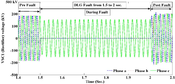
Fig 2.15 Three phase voltage at VSC1 (Rectifier) side with respect to DLG fault ... 47
Fig 2.16 Three phase current at VSC1 (Rectifier) side with respect to DLG fault ... 48
Fig 2.17 DC line voltage with respect to DLG fault ... 48
Fig 2.18 DC line current with respect to DLG fault... 49
Fig 2.19 VSC HVDC system ... 49
xi
Fig 2.21 Three phase current with respect to DLG fault ... 51
Fig 2.22 DC line voltage with respect to DLG fault ... 51
Fig 2.23 DC line current with respect to DLG fault on VSC1 side ... 52
Fig 3.1 Actual DC line current ... 57
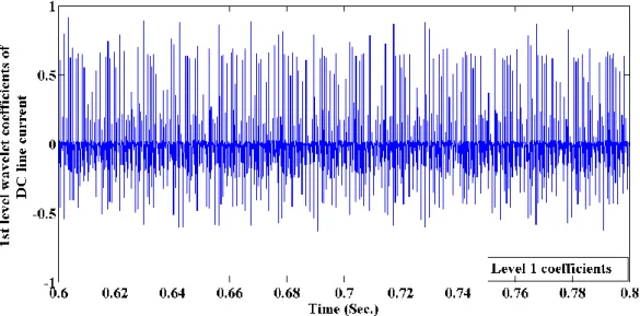
Fig 3.2 1st level wavelet coefficients of DC normal line current ... 58
Fig 3.3 2nd level wavelet coefficients of DC normal line current ... 58
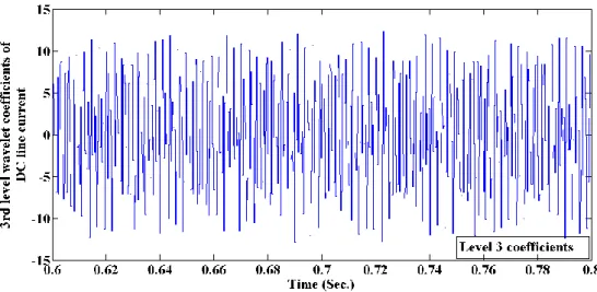
Fig 3.4 3rd level wavelet coefficients of DC normal line current ... 59
Fig 3.5 4th level wavelet coefficients of DC normal line current ... 59
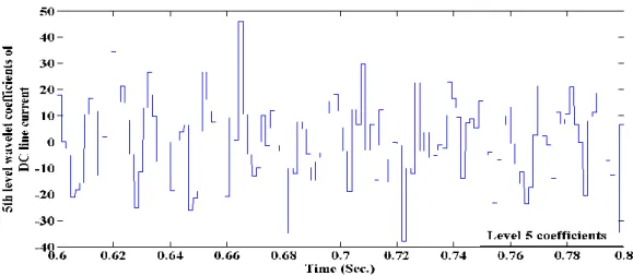
Fig 3.6 5th level wavelet coefficients of DC normal line current ... 60
Fig 3.7 Actual DC line Current for 80% power transfer ... 60
Fig 3.8 1st level wavelet coefficients of DC normal line current………...61
Fig 3.9 2nd level wavelet coefficients of DC normal line current………..61
Fig 3.10 3rd level wavelet coefficients of DC normal line current……….62
Fig 3.11 4th level wavelet coefficients of DC normal line current……….62
Fig 3.12 5th level wavelet coefficients of DC normal line current……….63
Fig 3.13 Actual DC line current for 50% power transfer………..63
Fig 3.14 1st level wavelet coefficients of DC normal line current……….64
Fig 3.15 2nd level wavelet coefficients of DC normal line current………64
Fig 3.16 3rd level wavelet coefficients of DC normal line current……….65
Fig 3.17 4th level wavelet coefficients of DC normal line current……….65
Fig 3.18 5th level wavelet coefficients of DC normal line current……….66
Fig 3.19 Actual DC line current for DC fault at 50 km……….67
Fig 3.20 5th level wavelet coefficients of DC line current for DC fault at 50 km ... 67
Fig 3.21 Actual DC line current for DC fault at 100 km ... 68
Fig 3.22 5th level wavelet coefficients of DC line current for DC fault at 100 km ... 68
Fig 3.23 Actual DC line current for 150 km fault ... 69
xii
Fig 3.25 5th level wavelet coefficients of DC line current for DC fault at 200 km ... 70
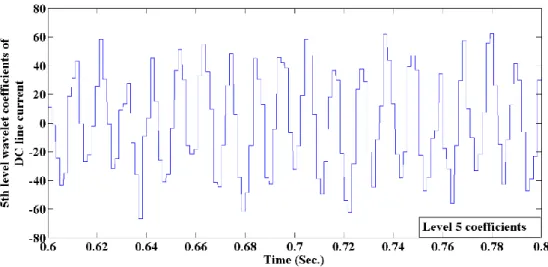
Fig 3.26 5th level wavelet coefficients of DC line current for DC fault at 250 km ... 71
Fig 3.27 Actual DC line current for SLG fault at VSC1 side ... 74
Fig 3.28 5th level wavelet coefficients of DC line current for SLG fault at VSC1 side ... 74
Fig 3.29 5th level wavelet coefficients of DC line current for LL fault at VSC1 side ... 75
Fig 3.30 5th level wavelet coefficients of DC line current for DLG fault at VSC1 side ... 75
Fig 3.31 5th level wavelet coefficients of DC line current for LLL fault at VSC1 side ... 76
Fig 3.32 Actual DC line current for SLG fault at VSC1 in VSC-HVDC………..78
Fig 3.33 5th level wavelet coefficients of DC line current for SLG fault at VSC1……78
Fig 3.34 5th level wavelet coefficients of DC line current for LL fault at VSC1……...79
Fig 3.35 5th level wavelet coefficients of DC line current for DLG fault at VSC1……79
Fig 3.36 5th level wavelet coefficients of DC line current for LLL fault at VSC1…….80
Fig 4.1 Training structure of ANN ... ….82
Fig 4.2 Proposed neural network structure ... 83
Fig 4.3 Three phase voltage at VSC1 side with respect to SLG, DLG, LL faults ... 86
Fig 4.4 Three phase current at VSC1 side with respect to SLG, DLG, LL faults ... 87
Fig 4.5 DC link voltage with respect to SLG, DLG, LL faults ... 87
Fig 4.6 DC link current with respect to SLG, DLG, LL faults ... 88
Fig 4.7ANN fault detection and classification with respect to SLG, DLG, LL faults .. 88
Fig 4.8 Three phase line voltage with respect to DC fault ... 89
Fig 4.9 Three phase current with respect to DC fault ... 89
Fig 4.10 DC line voltage with respect to DC fault ... 90
Fig 4.11 DC line current with respect to DC fault ... 90
Fig 4.12 ANN fault detection and classification with respect to DC fault... 91
Fig 4.13 Three phase voltage with respect to SLG fault at VSC2 side ... 91
Fig 4.14 Three phase current with respect to SLG fault at VSC2 side ... 92
xiii
Fig 4.16 DC line current with respect to SLG fault at VSC2 side ... 93
Fig 4.17 ANN fault detection and classification with respect to SLG fault at VSC2 side ... 93
Fig 4.18 ANN mean square error curve ... 95
Fig 4.19 ANN gradient curve ... 95
Fig 4.20 ANN epoch mu curve ... 95
Fig 5.1 Magnitude of voltage of the dq-axis component waveform during a DLG fault at VSC1 side of the HVDC system ... 100
Fig 5.2 Magnitude of current of the dq-axis component waveform during a DLG fault at VSC1 side of the HVDC system ... 101
Fig 5.3 Fuzzy Inference Engine for fault classification of VSC-HVDC system ... 103
Fig 5.4 Fuzzification and Defuzzification memberships ... 104
Fig 5.5 Surface diagram of FIE for fault classification of VSC – HVDC system ... 105
Fig 5.6 Verification of the developed FIE in MATLAB... 106
Fig 5.7 FIE output corresponding to the 80% power transfer from VSC1 to VSC2 ... 107
Fig 5.8 Performance comparison of different defuzzification methods ... 108
Fig 5.9 Performance of the developed FIE for various power transfer capacity ... 109
Fig 5.10 Conversion of voltages and currents through gain block... 111
Fig 5.11 Output waveform of the VSC HVDC system during single line to ground fault at phase a in VSC1 side ... 112
Fig 5.12 Output waveform of the VSC HVDC system during single line to ground fault at phase b in VSC1 side... 113
Fig 5.13 Voltages of phase a b c with & without gain and dq axis voltage of VSC1 ... 114
Fig 5.14 Voltages of phase a b c with & without gain and dq axis voltage of VSC2 ... 114
Fig 5.15 DC line current (fault at VSC2 side)... 115
Fig 5.16 Voltages of phase a b c with & without gain and dq axis voltage of VSC1 ... 115
Fig 5.17 Voltages of phase a b c with & without gain and dq axis voltage of VSC2 ... 116
Fig 5.18 DC line current ... 116
xiv
Fig 5.20 Fault analysis for 50% power transfer ... 120
Fig 5.21 Fault analysis for 30% power transfer ... 120
Fig 5.22 Fault analysis of DC line current for 30%, 50%, 80% and 100% power transfer .. 121
Fig 5.23 Flow chart for classification algorithm ... 122
Fig 5.24 Fuzzy inference engine for fault classification ... 123
Fig 5.25 FIE rules produce crisp output ... 126
Fig 5.26 Fault status (VSC1) vs Fault index ... 129
Fig 5.27 Fault status (VSC2) vs Fault index ... 130
Fig 5.28 Fault status (DC) vs Fault index ... 130
Fig 5.29 Fault status (La) vs Fault index ... 131
Fig 5.30 Fault status (Lb) vs Fault index ... 131
Fig 5.31 Fault status (Lc) vs Fault index ... 132
Fig 5.32 Fault status (G) vs Fault index ... 132
Fig 5.33 Fault status vs Fault index... 133
Fig 5.34 Modified FIE ... 134
Fig 5.35 Conversion of voltages through gain block for new Vdqabb ... 135
Fig 5.36 Modified dq axis voltage ... 135
Fig 5.37 Scattering plot of dq axis voltages ... 137
Fig. 5.38 Performance chart of modified FIE ... 139
Fig 6.1 MTDC model ... 144
Fig 6.2 Conversion of voltages through gain block for VdqWTabc ... 145
Fig 6.3 Conversion of voltages through gain block for VdqWTabb ... 146
Fig 6.4 Conversion of voltages through gain block for IdqWTabc ... 146
Fig 6.5 Output waveform of the MTDC system during single line to ground fault at phase A in wind turbine 1 side (VdqWT1abc) ... 147
Fig 6.6 Output waveform of the MTDC system during single line to ground fault at phase A in wind turbine 1 side (VdqWT1abb) ... 147
xv
Fig 6.7 Output waveform of the MTDC system during single line to ground fault at
phase A in wind turbine 1 side (IdqWT1abb) ... 148
Fig 6.8 Fuzzy inference engine for fault classification of MTDC ... 152
Fig 6.9 Range of memberships for Vdqabc of WT1 and WT2 ... 153
Fig 6.10 Range of memberships for Vdqabb of WT1 and WT2 ... 153
Fig 6.11 Range of memberships for Idqabc of WT1 and WT2... 153
Fig 6.12 FIE rules produce crisp output for MTDC ... 155
xvi
List of Tables
Table 1.1 Rating of the HVDC components ……….12
Table 1.2 Different faults scenarios in HVDC system………...13
Table 2.1 Merits and demerits of HVDC ... 17
Table 2.2 Comparison of CSC vs VSC ... 19
Table 2.3 HVDC Projects... 25
Table 3.1 Absolute maximum values of the wavelet coefficients of the DC line current for different power transfer ………66
Table 3.2 Absolute maximum values of the Wavelet Coefficients of the DC line current .... 72
Table 3.3 The wavelet entropies of DC line current at various fault locations ... 73
Table 3.4 Absolute maximum value of the Wavelet Coefficients of the DC line current for AC fault conditions ... 76
Table 3.5 The wavelet entropies of three phases AC line current... 77
Table 4.1 Fault conditions considered... 86
Table 4.2 Summary of ANN algorithm generated firing Angle (Alpha) ... 94
Table 5.1 Simulation results of the VSC-HVDC system during five different types of faults (Maximum Power: 100%) ... 102
Table 5.2 Fault index table ... 104
Table 5.3 FIE output corresponding to the 50% power transfer from VSC1 to VSC2 ... 108
Table 5.4 Fault index table for various faults in the HVDC System ... 118
Table 5.5 VSC HVDC Fault Data at 100% Power Transfer ... 119
Table 5.6 Fuzzy variable in the antecedent Parts ... 123
Table 5.7 Simulation result of Mamdani and Sugeno methods for 100% power transfer.... 127
Table 5.8 FIE output corresponding to the 30% power transfer form VSC1 to VSC2 ... 129
Table 5.9 Performance evaluation of modified FIE on fault index 77 ... 138
xvii
Table 6.1 Fault index table for various faults in the HVDC System ... 149
Table 6.2 MTDC fault data power transfer (WT1=1050 W, WT2=950 W) ... 150
Table 6.3 MTDC fault data power transfer (WT1=800 W, WT2=650 W) ... 151
Table 6.4 Fuzzy variable in the antecedent parts for MTDC ... 152
xviii
List of Symbols
cA Approximation coefficient cD Details coefficient db4 Daubechies wavelet P Active power Q Reactive power S Signal Si Coefficients of signalE(k) Instantaneous difference between expected and actual
target value
E(s) Shannon entropy
N Number of sample Data
ai Expected value
bi Measured value
η Gain parameter
δi Updated error
Wij Connection weight of neural network
P Input vector
O Desired output
Vdq Magnitude of dq-axis value of voltage of three phase
signal
Idq Magnitude of dq-axis value of current of three phase
signal
VSC1 Source 1 side (Rectifier)
VSC2 Source 2 side (Inverter)
1
Chapter 1
Introduction
1.1 Background
In 1954, Gotland 1, the first commercial installation of a high voltage direct current (HVDC) system was the beginning of HVDC projects in the world. From there the growth of the world wide HVDC transmission capacity was significant as shown in Fig 1.1[1]. To transmit large quantities of power over long distances by overhead transmission lines or submarine cables, HVDC is the best technology [4]. AC has been the preferred global platform for electrical transmission to homes and businesses for the past 100 years. However high voltage AC transmission has some limitations, starting with transmission capacity and distance constraints, and the impossibility of directly connecting two AC power networks of different frequencies. HVDC is now the method of choice for sub-sea electrical transmission and the interconnection of asynchronous AC grids, providing efficient, stable transmission and control capability. HVDC is also the technology of choice for long distances with low electrical losses. That makes it a key technology in overcoming problems with renewable generation such as wind, solar and hydro in that these resources are seldom located near population centers that need them [4]. In HVDC systems, electric power is taken from a three phase AC network and then converts it to DC in a converter station. The DC power is then transmitted to the receiving point by an overhead line or cable and this is converted back to AC in another converter station for the receiving AC network.
2
Fig 1.1 Growth in global HVDC capacity (Projects up to 2016) [1]
The global wind 2014 report from Global Wind Market Council (GWMC) shows that 2014 was a record year for the wind industry as annual installation crossed the 50 GW mark for the first time [2]. More than 51 GW of new wind power capacity was brought on line, a sharp rise in comparison to 2013, when global installations were just over 35.6 GW. The previous record was set in 2012 when over 45 GW of new capacity was installed globally. The new global total at the end of 2014 was 369.6 GW, representing cumulative market growth of more than 16%, which is lower than the average growth rate over the last 10 years (2005-2014) of almost 23%. At the end of 2013, the expectations for the wind power market growth were uncertain, as continued economic slowdown in Europe and political uncertainty in the US made it difficult to make projections for 2014. China, the largest overall market for wind since 2009, had another remarkable year, and retained the top spot in 2014. Installations in Asia again led global markets, with Europe reliably in the second spot, and North America a distant third. Fig 1.2 shows the global annual installed wind capacity 1997-2014 and Fig 1.3 shows the global cumulative installed wind capacity 1997-2014[2].
3
Fig 1.2 Global annual installed wind capacity 1997-2014 [2]
Fig 1.3 Global cumulative installed wind capacity 1997-2014 [2]
In Asian countries in terms of annual installations, China maintained its leadership position in the year 2014. China added just over 23 GW of new capacity in 2014, the highest annual number for any country ever. This is a significant gain over 2013 figures when China installed 16 GW of new capacity. China aims to nearly double its wind capacity to 200 GW by the end of 2020. India is the second largest wind market in Asia, presenting substantial opportunities for both international and domestic players. The Indian wind sector has struggled in the last couple of years to repeat the strong market performance of 2011 when over 3 GW was installed, and 2014 seems to signal the onset of a recovery phase. While the rest of Asia did not make much progress in 2014, there are some favorable signs on the horizon. The Japanese market saw new installations of 130.4 MW in 2014 to reach a cumulative capacity of 2,788.5 MW. South Korea still has “green growth” as one of its national development priorities, wind power is still a
4
relatively small energy generation technology, with 47.2 MW of new installations in 2014, bringing total installed capacity to just over 608 MW. Pakistan commissioned 149.5 MW of large-scale commercial wind farms in 2014, with total installed capacity reaching 255.5 MW by the end of the year. The Philippines saw 150 MW of new capacity installed in 2014, bringing its total installed capacity up to 216 MW. Taiwan added 18 MW of new capacity, bringing its total installed capacity to just over 632 MW. As for the rest of Asia, expect new projects to come online in Thailand and Vietnam in 2015.
In North America, 1,871 MW of new wind capacity came online in Canada in 2014, making it the sixth largest market globally. Compared to 1,609 MW in 2013, Canada’s wind power market saw significant growth in 2014, its best year ever. Canada finished 2014 with nearly 9,700 MW of total installed capacity, supplying approximately 4% of Canada’s electricity demand. The US is the second largest market in terms of total installed capacity after China today. Mexico installed 633.7 MW of new capacity to reach a total of 2,551 MW by the end of 2014.
In Europe, during 2014 12,858 MW of wind power was installed across Europe, with the European Union (EU-28) member states accounting for 11,829 MW of the total. The European wind energy industry installed more new capacity than gas and coal combined in 2014. Across the EU-28 states the wind industry connected a total of 11,829 MW to the grid with coal and gas adding 3,305 MW and 2,338 MW respectively. The total installed offshore wind capacity for Europe now stands at 8,045 MW in 74 offshore wind farms in 11 European countries. Almost 1.5 GW of offshore wind was installed in 2014, 5.3% less than 2013. The UK has the largest offshore wind capacity in Europe- 4,494 MW accounting for over 55% of all installations. Denmark follows with 1,271 MW or 15.8% of the market share. Germany is third with a 13% share, followed by Belgium with 713 MW for an 8.8% share, the Netherlands with 247 MW with a 3.1%
5
share, Sweden with 212 MW and a 2.6% share, and others with less than 1% share including Finland with 26 MW, Ireland with 25 MW, Spain with 5 MW, Norway with 2 MW and Portugal with 2 MW installed capacity.
South Africa has taken off in 2014, installing 560 MW of new capacity, for a cumulative capacity of 570 MW. This is just the beginning of the wind market in the country. The Australian market added 567 MW in 2014 (down from 655 MW in 2013), bringing its total installed capacity up to 3,806 MW. According to recent research conducted by the Clean Energy Council, 14.76% of Australia’s electricity came from renewable sources in 2013 [2]. By 2020, EWEA targets to develop 40GW installed capacity for offshore wind in Europe [3]. The structure of the system is shown in the Fig 1.4 [5].
Fig 1.4 HVDC system structure [5]
1.2 Research motivations and objectives
Fault analysis plays a critical role in the protection of any system. For safe operation of HVDC systems, the detection and fast clearance of faults in the HVDC lines are very important. In HVDC systems, AC side faults on the rectifier and inverter sides and DC faults on the line can occur. It is necessary to investigate the fault detection and fault classification for better protection of the system.
The main objective of the research is to demonstrate and assess different approaches to detect and classify different faults in the HVDC system. The following signal processing techniques are considered:
6
(i) Wavelet transformation
(ii) Artificial neural network (iii) Fuzzy logic
The reasons for chosen above three techniques are explained here. The major advantage of wavelet transform is the ability to perform local analysis i.e. to analyze a localized area of a larger signal. The fault generated transient signal comprises of high frequency and low frequency components. High frequency signals high light the instant of fault occurrence. By applying multiband filters, high frequency signals can be extracted and used to detect the time where a fault generated. Authors in [56] clearly mentioned the importance of the wavelet transform technology in power quality disturbance. This paper indicates that many studies have been conducted how to extract features using wavelet transform. The study mentioned in [56] are proposing of a squared wavelet transform coefficients at different scale, preprocessed wavelet coefficients as inputs to a refined neuro-fuzzy network etc. Therefore adopting directly the wavelet transform for the fault analysis of HVDC system is a genuine approach.
The investigation of fault analysis of HVDC system based on artificial neural network (ANN) is explained here. Neural network is the most fast iteration technique with back propagation algorithm. Authors in [80] mentioned that the ANN can deal with hard classification problem and neural network is a special type of neural network that is widely used in the classification application. The neural network has a fast training process, an inherent parallel structure and guaranteed optimal classification performance if a sufficiently large training set is provided. Neural network is usually executed with more numbers inputs, hidden layer and output layers. In this research work the developed neural network is based on one input layer, one output layer and with five hidden layer neurons which make the system computation is faster.
7
Again the selection of fuzzy logic is explained here for the HVDC fault analysis. Fuzzy logic is a better tool dealing with a imprecise data set. The concept of imprecise is fuzzy logic. Fuzzy set can be manipulated with degree of membership function and it is a linguistic variable approach. This means variable whose values are words rather than numbers. An author in [89-90] shows the application of fuzzy logic in the area of fault classification. By considering all the above factors it is decided to choose fuzzy logic approach for the fault analysis of HVDC system.
1.3 Research contributions and developments
The research work here to achieve the objectives mentioned in the previous section has led to the following contributions and developments:
(i) Literature review dealing with the following
Fault detection and classification in HVDC systems using wavelet
transformation.
Training of the artificial neural network for detection and classification of faults.
Designing the steps of developing a Fuzzy Inference Engine for complete classification of HVDC system faults.
Fault analysis of Multi-Terminal HVDC systems.
(ii) Fault analysis using Wavelet Transform
This research shows the importance of wavelet transformation in the fault analysis of LCC HVDC systems. Wavelet transformation effectively proved that it can detect the abrupt changes of the signal indicative of a fault.
8
DC faults in the system at various distances have been detected successfully.
5th level wavelet coefficients have been used to detect the DC faults at various
locations (50km, 100km, 150km, 200km, and 250km) in the LCC HVDC system.
The detection of the DC faults at various distances has been achieved by using wavelet coefficients.
For more accurate classification of DC faults at various locations, the wavelet entropy principle has been applied.
AC faults in the system have been detected successfully.
In the AC fault analysis, symmetrical and unsymmetrical faults such as single line to ground (SLG), line to line (LL), double lines to ground (DLG) and triple line faults (LLL) are considered specifically.
5th level wavelet coefficients have been used to detect the AC faults in the LCC HVDC system.
The classification of the AC faults has been done by using wavelet coefficients and wavelet entropy.
(iii) Fault analysis using Artificial Neural Network
In this analysis the detection and classification of different faults that can occur in a LCC-HVDC system, with the help of artificial neural network (ANN) training algorithm techniques have been done.
Five neurons in the hidden layer and a set of training data for input and output layers.
Single-line to ground, double-line to ground, line-line, HVDC transmission line (DC link) and single line to ground faults on the load end (inverter side) are examined.
9
A set of simulation results are provided to show the effectiveness of the ANN technique subjected to developed fault conditions.
After detailed investigation an algorithm was developed that provided the trade-off with large input data size and minimal number of neurons in the hidden layer without compromising the accuracy.
(iv) Fault analysis using Fuzzy Logic
This research presents the detection and classification of different faults that can occur in the VSC1 (rectifier side) and VSC1 & VSC2 side of the VSC-HVDC system with the help of a fuzzy logic method.
In phase 1 of this research, single line to ground fault, double line to ground fault, triple line to ground fault and line to line ground fault has been specifically considered.
A fault index table has been developed for the fault analysis of a VSC1 of VSC-HVDC system.
A Fuzzy Inference Engine has been developed for the fault analysis of a VSC1 of VSC-HVDC system.
Results prove that the developed FIE identifies the AC faults occurring in the VSC1 side and DC faults successfully.
In phase 2 of this research, 21 faults have been specifically considered for detection and classification.
A fault classification strategy based on the dq transformation has been proposed.
A fault index table has been developed by using binary coding system.
10
A Fuzzy Inference Engine with three inputs has been developed. The accuracy of this system was 99%.
A Fuzzy Inference Engine has been developed based on the Mamdani [109] and Sugeno [110] approach.
A Fuzzy Inference Engine has been modified with five inputs. The accuracy of this system was 100%.
(v) Fault analysis of Multi-Terminal HVDC system
In this part of the research, 20 faults have been specifically considered for identification and classification.
A fault classification strategy based on the dq transformation has been proposed.
A fault index table has been developed by a using binary coding system.
Different fault data table has been generated for various power transfer.
A Fuzzy Inference Engine with six inputs has been developed. The accuracy of this system was 100%.
1.4 HVDC model and measurements
In this research report the LCC/VSC HVDC model has been used for the analysis. In chapter 3 wavelet analysis has been applied to both LCC and VSC model. But in chapter 4 it is essential to investigate only LCC HVDC model. The reason is mentioned in chapter 4. In chapter 5 focused on VSC HVDC model and chapter 6 is based on muti terminal HVDC model. Throughout the research sensors has been connected in the same location for the measurements and its demonstration is shown in Fig 1.5.
11
Fig 1.5 Demonstration of measurements from HVDC model
As shown in the figure above, three phase measurements has been connected to get the data for the analysis. The measurement block will give three phase voltages and currents. In the same way measurement block has been connected in the DC line/cable to get the data for the analysis. After getting the data from the simulation of MATLAB model, it is processed according to the application.
The objective of the research work is not the modeling of the HVDC system. This means generator, converter, cable and inverter have not been modeled. Therefore the default model from the MATLAB/Simulink model has been taken for the analysis. These models are used for the investigation of the various signal processing techniques for fault analysis in HVDC network. The ratings of the components of LCC/VSC model are shown in the Table 1.1.
12
Table 1.1 Rating of the HVDC components LCC HVDC
Power P 1000 MW ( 500 kV, 2 kA)
Source S1 500 kV, 5000 MVA, 60 Hz
Source S2 345 kV, 10000 MVA, 50 Hz
Smoothing reactor 0.5 H
DC line Length 300 km, Resistance per unit length = 0.015 ohms per
km, Inductance per unit length = 0.792e-3 H/km, Capacitance per unit length = 14.4e-9 F/km
Three-Phase Transformer 1200 MVA, 60/50 Hz AC Filter 600 Mvar, 60/50 Hz VSC HVDC Source S1 230 kV, 2000 MVA, 50 Hz Source S2 230 kV, 2000 MVA, 50 Hz VSC Converter 200 MVA, (+/- 100 kV DC)
Cable Length 75 km, Resistance per unit length = 1.3900e-002
ohms per km, Inductance per unit length = 1.5900e-004 H/km, Capacitance per unit length = 2.3100e-007 F/km Three-phase
Transformer
200 MVA, 230:100 kV, 50 Hz
AC Filter 40 Mvar, 100 kV
Different faults have been considered in this research and all the type of faults is shown in the Table 1.2.
13
Table 1.2 Different faults scenarios in HVDC system
Faults Representation in Thesis
Single line to ground (a) -SLG La-G
Single line to ground (b) -SLG Lb-G
Single line to ground (c) -SLG Lc-G
Double line (a-b) - LL La -Lb
Double line (b-c) - LL Lb -Lc
Double line (a-c) - LL La -Lc
Double line to ground (a-b) -DLG La -Lb-G
Double line to ground (b-c) -DLG Lb -Lc-G
Double line to ground(a-c) -DLG La -Lc-G
Triple line to ground(a-b-c) -LLLG La-Lb-Lc-G
DC line/cable fault, open circuit DC
1.5 Outline of the Thesis
This research report is divided into seven chapters.
Chapter One
The first chapter contains a brief introduction to the energy sector and the importance of HVDC in this sector. An overview of HVDC technologies is also presented.
Chapter Two
In Chapter 2 a literature review of HVDC systems and associates fault analysis is presented. Initially the general aspects of HVDC systems are presented and then the detailed reviews of the importance of the protection of the system are considered. Then a detailed review of wavelet based fault analysis, artificial neural network
14
based fault analysis, fuzzy logic based fault analysis and multi terminal HVDC system fault analysis are presented. An explanation of fault analysis of HVDC systems is then given. Initially, the LCC HVDC system model and its dynamic behavior are presented. The VSC HVDC system is considered together with its dynamic behavior. At the end of this chapter, the scope of the research is presented.
Chapter Three
Chapter 3 deals with the application of the wavelet transform in the area of fault analysis of a LCC and VSC HVDC system. Wavelet based analysis has been done under AC fault and DC fault scenarios. After the wavelet based analysis has been applied, wavelet entropy is applied to the classification of the faults in the system.
Chapter Four
Chapter four deals with the application of an artificial neural network in the area of LCC HVDC system fault analysis. The training of the neural network with a back-propagation algorithm is presented.
Chapter Five
This chapter deals with fuzzy logic and its application in the area of VSC HVDC system analysis. Based on the input data a Fuzzy Inference Engine for fault classification has been developed and the performance of this engine is also presented here.
Chapter Six
Chapter six deals with the fault analysis of a multi-terminal HVDC system using fuzzy logic. This chapter discusses the generation of the data table and the fault index, and the development of a Fuzzy Inference Engine for the wind farm side of a multi-terminal HVDC system.
15
Chapter Seven
The conclusions of this research work are presented in the final chapter. Future work is also proposed.
16
Chapter 2
Literature Review
2.1 General Aspects of HVDC
Future offshore wind farms will mostly be located far away from the shore, and have to be connected to the grid point of common coupling (PCC) via undersea cables over long distances. Two types of technologies are available to integrate offshore wind farms to the onshore mainland grid. One is HVAC (High voltage alternating current) and the other is HVDC (High voltage direct current). In comparison to HVDC transmission, an HVAC cable is characterized by its significant large shunt capacitance. This may cause a large charging current carrying reactive power flows and may impact the stability of the system. Therefore reactive power compensation becomes a natural part of the scheme and must be carefully designed to guarantee the system voltage stability [6]. The main advantage of HVAC system is that it has been already successfully used and for a higher power or a longer distance, the use of HVDC for transmission is necessary. The advantages and disadvantages of HVDC transmission are shown in Table 2.1. The use of HVDC technology as an alternative option for power transmission rests on the benefits in terms of economic and reliability issues and environmental impact. The thyristor-based Line Commutated Converters (LCCs) were introduced during the 1970s [8]. LCC is the converter that can be built with highest power rating and hence is the best solution for bulk power transmission. Another advantage of LCC is the low losses, typically 0.7% per converter [8].
17
Table 2.1 Merits and demerits of HVDC
Merits Demerits
No reactive power loss No stability problem No charging current
No Skin and Ferranti effect Power control is possible
Requires less space compared to AC for same voltage rating and size.
Ground can be used as return conductor Less Corona loss and radio interference.
Cost of terminal equipment is high Introduction of harmonics
Blocking of reactive power Point-to-point transmission Limited overload capacity
Significant reactive power requirements at the converter terminals.
The largest disadvantage is that both the inverter and the rectifier absorb a varying amount of reactive power from the grid. The LCC will also need an AC voltage source at each terminal to be able to achieve with commutation. In order to minimize the harmonic content, the standard LCC design consists of with two 6-pulse bridges in parallel on the AC side and in series on the DC side. The two bridges are phase shifted 30 degrees on the AC side, using transformers [8]. In 1954 the first commercial HVDC connection was installed between the main land of Sweden and the island of Gotland. In the LCC converter the current is always lagging the voltage due to the control angle of the thyristors; hence these converters consume reactive power. For this reason capacitor banks or STATCOM devices are part of the structure [9-10]. The drawbacks of LCC are that the converters absorb reactive power (50%-60% of active power), harmonic filters are needed to filter AC harmonics.
18
The Classical Voltage Source Converter (VSC) utilizing Insulated Gate Bipolar Transistors (IGBTs) for HVDC applications was introduced in 1997 as the ABB concept HVDC Light [11]. Classical VSC for HVDC applications is based on two-level or three-level converters [11]. With this concept it is not possible to adjust the voltage magnitude at the AC terminals, but the voltage can be either ± V with two-level or ± V or zero voltage with three-level VSC [12]. Pulse Width Modulation (PWM) is used to approximate the desired voltage waveform and the difference between the desired and implemented waveform is an unwanted distortion which has to be filtered [12]. Because IGBTs have limited voltage blocking capability, they need to be connected in series in two-level and three-level VSCs [11]. In order to increase the voltage across each semiconductor, series connected IGBTs must be switched absolutely simultaneously. This requires sophisticated gate drive circuits to enforce voltage sharing under all conditions [13]. With VSCs, both active power flow and reactive power flow can be controlled independently, and accordingly no reactive compensation is needed. A VSC station is therefore more compact than a LCC station as the harmonic filters are smaller and no capacitor banks are needed [8]. Other advantages with the VSC is that the converter can be connected to weak systems and even to networks lacking generation [8], and as no phase shift is needed, the VSC can use ordinary transformers. A disadvantage is that the VSC has larger losses than LCC, typically 1.7% per converter. Using LCC, the current direction is fixed and power reversal is achieves by changing the voltage polarity [8]. With VSCs, power reversal is achieves by changing of the current direction. This makes the VSC technology more suitable for a DC grid application [8]. Cross-linked polyethene (XLPE) cables can be used with VSCs but cannot handle the stress from a polarity change. XLPE cables are advantageous as they are less costly, lighter, and smaller in diameter than traditional mass impregnated cables [14]. The power reversal with VSCs can be done gradually because the full range of
19
active power is available, even zero active power can be combined with a positive or negative reactive power. Because both active and reactive power can be combined with positive and negative values, the converter is said to operate in all four quadrants of the P-Q plane [15]. LCCs normally have a minimum active power output 5% below rated power. This makes VSC more favorable for power transmission with varying power e.g. power generated from a wind farm. But an advantage with LCC HVDC is that DC pole to pole short circuit faults can be cleared in the converter station. This is not the case with classical VSC HVDC where in most cases the fault currents must be suppressed by opening the AC breaker feeding the converter [13]. VSC-HVDC is particularly suitable for the connection of distant offshore wind farms to the AC grid due to its attractive features of reactive power support for the wind farm, small size of filters and black-start capability [16].VSC HVDC can change the direction of its power flow without reversing the polarity of the voltage of the DC cables. This feature makes it more suitable for Multi-Terminal HVDC than line commutated HVDC [16]. Again another comparison of Current Source Converter (CSC) and VSC is shown in Table 2.2.
Table 2.2 Comparison of CSC vs VSC
CSC VSC
Inductor is used in DC side Constant current
Higher losses
Fast accurate control Larger and more expensive
More fault tolerant and more reliable Simpler control
Capacitors is used in DC side Constant voltage
More efficient Slow control
Smaller and less expensive
Less fault tolerant and less reliable Complex control
20
VSC transmission uses PWM modulation with a switching frequency of several kilohertz to synthesize a sinusoidal voltage on the AC side. The major drawback of the VSC technology is the high-converter loss that is caused mainly by switching losses that depend on the switching frequency of the semiconductor devices. The above section has given a brief idea about the general aspect of HVDC system. As mentioned earlier two basic converter technologies are used in modern HVDC transmission system. These are Line Commutated current source Converters (LCC) and self-commutated voltage source converters (VSC) which will be discussed in the following section.
2.1.1 LCC HVDC
Conventional HVDC transmission employs line-commutated, Current-Source Converters (CSC) with thyristor valves. Such converters require a synchronous voltage source in order to operate. The basic building block used for HVDC conversion is the three-phase, full-wave bridge referred to as a 6-pulse or Gratez bridge [17]. Fig 2.1 shows the basic structure of LCC HVDC system [18]. As shown in Fig. 2.1, where three phase AC system is connected to the converter which will convert AC to DC and this DC power will reach to the second converter. Again the DC power will convert into AC power. The structure is known as monopolar HVDC system. This having only one conductor as opposed as two conductors and ground is normally used as a return path.
21 2.1.2 VSC HVDC
HVDC transmission with VSC converters can be beneficial to overall system performance. VSC converter technology can rapidly control both active and reactive power independently of one another. Reactive power can also be controlled at each terminal independent of the DC transmission voltage level. This control capability gives total flexibility to place converters anywhere in the AC network since there is no restriction on minimum network short circuit capacity. Self-commutation with VSC even permits black start, i.e., the converter can be used to synthesize a balanced set of three phase voltages as in a virtual synchronous generator. The dynamic support of the ac voltage at each converter terminal improves the voltage stability and can increase the transfer capability of the sending and receiving end AC systems thereby improving the transfer capability of the DC link [17]. A typical VSC HVDC configuration is shown in Fig 2.2 [19]. As shown in the figure a 230 kV, AC power is connected to the converter through the transformer. This converts AC power into the DC and the rating is 320 kV, 1.3 kA. The DC power is converts into AC power and through the transformer this AC power is supplied at 400 kV to the grid.
Fig 2.2 Typical Bipolar VSC HVDC configuration [19]
Fig 2.3 compares the Three Gorges-Shanghai power transmission as an AC and DC transmission system. The top line shows two 3000 MW HVDC lines, compared to the
22
five 500 kV AC lines (below) that would have been needed if AC transmission had been selected to deliver the same amount of power. HVDC transmission systems clearly have far smaller footprints than AC systems [20].
Fig 2.3 Comparisons of HVDC and HVAC [20]
HVDC transmission lines cost less than an AC line for the same transmission capacity. However, it is also true that HVDC terminal stations are more expensive due to the fact that they must perform the conversion from AC to DC, and DC to AC. But over a certain distance, the so called, “break-even distance” (approx. 600-800 km), the HVDC alternative will always provide the lowest cost [20]. Fig 2.4 shows a cost comparison of AC and DC transmission system for the Nelson River Bipole 1 [21].
23 2.1.3 Multi-Terminal HVDC
The most common configuration of an HVDC link consists of two terminal back to back converter stations connected by an overhead power line or undersea cable. An example is the 2000 MW Quebec to New England Transmission System opened in 1992, which is currently the largest multi-terminal system. Such systems are difficult to realize using Line Commutated Converters because reversals of power are affected by reversing the polarity of DC voltage, which affects all converters to the system [22]. Fig 2.5 shows a typical MTDC configuration [23]. This configuration consists of three converters. A wind farm (WF) is connected to the first converter for AC to DC conversion. This converter is known as Sending End Converter (SEC). After the AC-DC conversion, DC power is transferred through the cable to the two converters known as Receiving End Converter 1(REC1) and Receiving End Converter 2 (REC2) respectively. Again DC power is converted to AC and connects to the AC grid through the filter and transformer.
Fig 2.5 Typical MTDC configuration [23]
2.1.4 HVDC projects in the world
The world’s first commercial HVDC subsea power link, Gotland 1, connected main land Sweden to the island of Gotland and was developed by the company ASEA, ABB’s predecessor in 1954. From there 170 HVDC projects have been installed around
24
the world by ABB, 41 projects are installed by Siemens. A number of projects were also developed by Alstom. A map of the ABB projects is shown in Fig 2.6 [24].
Fig 2.6 Worlds HVDC projects from ABB [24]
In the late 1990’s major new technologies are introduced in the form of HVDC light and HVDC plus. This technology was based on the development of IGBT devices in the converter and extruded cables with solid polymer insulation. Some HVDC projects are shown in Table 2.3.
25
Table 2.3 HVDC Projects
Projects Date Capacity Length
Biswanath-Agra, India 2014-2015 6000 MW, ± 800 kV 1728 km Xiluodu-Hanzhou, China 2013 6400 MW, ± 800 kV 1300 km East-West Interconnector, Ireland-UK 2012 500 MW, ± 200 kV 262 km Norned, Norway-Netherlands 2008 700 MW, ± 450 kV 580 km Neptune, USA 2007 660 MW, ± 500 kV 105km Estlink, Estonia-Finland 2006 350 MW, ± 150 kV 105 km Troll A, Norway 2004 2*40 MW, ± 60 kV 70 km Murraylink, Australia 2002 200 MW, ± 150 kV 176 km Directlink, Australia 2000 3*60 MW, ± 80 kV 59 km Skagerraki, Norway-Denmark 1976 275 MW, ± 250kV 240 km
Pacific Intertie, USA 1970 1440 MW, ± 400 kV 1362 km
Gotland, Sweden 1954 20 MW, ± 100kV 96 km
2.1.5 Future HVDC systems
To ensure high levels of supply in the future, power transportation corridors will have to increase their voltage and current carrying capabilities. The next generation will be focused on Ultra High Voltage Direct Current (UHVDC) technology. In 2010, ABB started research on UHVDC transmission system with a rated voltage of 1,100 kV DC [24]. Another development of a HVDC system is in the area of offshore projects, which are growing in terms of rated power and being located farther from the shore and the grid entry points. Capturing offshore wind energy with HVDC solutions is a big challenge but it will be the direction of future development. HVDC technology started
26
with point to point connection but nowadays it is developing towards multi-terminal converter systems. The heart of the HVDC system is a converter. Presently industrial research has been focused on the multilevel converter for power conversion with higher efficiency [25]. In conclusion, HVDC technology has advanced in recent years and bulk transmission for extremely long distances has reached levels of 8 GW using ± 800 kV UHVDC and ratings above 10 GW are envisioned within a few years [24].
2.2 Fault Analysis of HVDC
The LCC-HVDC is a sixty years old technology but development of VSC-HVDC is unlikely to replace LCC based HVDC power transmission in the near future [7]. At present, all of the installed VSC-HVDC systems are either back to back converters or are connected through underground cables. No overhead DC lines have been installed as of yet. This means that the absence of overhead DC lines greatly reduces the risk of DC faults. In the case of a cable-connected systems, a ground fault is almost always permanent [26] because of the cable break. Classical CSC HVDC naturally is able to withstand short circuit current due to the presence of DC inductors which helps in limiting the current during fault conditions [26]. When a fault occurs on the DC side of a VSC-HVDC system the IGBT’s lose control and the freewheeling diodes act as a bridge rectifier and feed the fault [26].
As in AC systems, the faults in a DC system are caused by (i) the malfunctioning of the equipment and controllers and (ii) the failure of insulation caused by external sources such as lightning, pollution etc. The faults have to be detected and the system has to be protected by switching and control action such that the disruption in the power transmission is minimized [7]. The various faults also cause stressing of the equipment due to over currents and over voltages [7].
Since the thyristors are only turn-on devices, the active power flow of CSC HVDC is controlled by adjusting the turn-on (firing) and the extinction time instant (overlap)
27
prior to commutation to another valve. Under transient conditions reactive power consumption is higher, but it can be compensated by filters and additional capacitors on the AC sides. The power flow is unidirectional and the reversal of the power flow direction requires a change in polarity of the system, which is a difficult task. The losses in one terminal are ≈ 0.7% at rated power. This technology is still advancing through the application of capacitor-commuted conversion and using the turned AC filters and active DC filters [27]. The high power devices, including IGBT form the basis of the VSC HVDC system. The use of Pulse-Width modulation (PWM) is also possible in this technology, so that only high-frequency harmonics are present and the filters can be considerably smaller. The VSC HVDC can provide a stiff DC voltage and large capacitors are used. VSC HVDC technology transmits active power and can provide the required amount of reactive power at both the power sending and the power receiving end. The losses in each VSC terminal are ≈ 1.6% [27].
As mentioned earlier, in the case of a DC-side fault, the diodes connected in parallel to the IGBT modules act as an uncontrolled rectifier, even if the IGBT’s are blocked. The short circuit current is limited only by the AC system [27]. The small DC-side inductance leads to a very high rate of rise of DC current. In addition, the DC capacitors discharge and add to the fault current [27]. The rate of rise of DC short-circuit current in VSC HVDC system is large compared to CSC based HVDC. The size of the DC capacitors in VSC is large and inductor size is small. The size of the DC inductor in VSC HVDC is small compared to CSC HVDC. During the DC-side fault, VSC HVDC control will be lost (due to diodes) and in CSC based HVDC, control can be achieved by using phase angle. To each technology, there are certain advantages and disadvantages. CSC HVDC is well established and has a higher power rating combined with lower losses. But a fault on the AC side can lead to commutation failure which results in a collapse of the DC line voltage. A CSC-based network is thus vulnerable to
28
AC side faults. A VSC based network, in turn is vulnerable to a DC side faults. Any DC side fault will result in a fault current with steeply increasing amplitude. CSC requires relatively strong AC sources and consumers reactive power at every terminal location. In contrast, a VSC based network could help to strengthen regions with weak AC systems by its independently controllable active and reactive power [27]. The types of faults possible on a HVDC system are as follows [26];
Positive line to ground fault( L+ - G) Negative line to ground fault(L- - G)
Positive line to negative line fault(L+ - L-)
Overcurrent
Overvoltage.
Line to Ground (L+ or L- - G): A line to ground fault occurs when the positive or negative line is shorted to ground and the faulted pole rapidly discharges the capacitor. This causes an imbalance of the DC link voltage between the positive and negative poles. As the voltage of the faulted line begins to fall, high currents flow from the capacitor as well as the AC grid. These high currents may damage the capacitors and the converter [26].
Line-to-Line (L+ - L-): A line-to-line fault on a cable connected system is likely to occur
on the cable. In an overhead system, line-to-line faults can be caused by an object falling across the positive and negative line; it may also occur in the event of the failure of a switching device causing the lines to short. This fault may be either temporary or permanent.The analyses of both thyristor-based HVDC and VSC HVDC are completely different in nature of the short circuit currents in the case of a fault on the DC side. In classic LCC HVDC, the DC side smoothing reactor has filtering tasks and protects the converter in case of faults. The size of the reactor has an effect on the duration of the short circuit current. The control system is also essential, having a limiting influence of
29
the short circuit current on the DC side. In the VSC HVDC concept, the anti-parallel diodes are an important part of the converter, which allows a reversal in the power transmission direction. This configuration plays an essential role in the event of a short circuit on the DC side, because of the uncontrollability of the diodes. In the case of a fault, the converter has to be tripped off by an AC circuit breaker to extinguish the arc. DC capacitors are additional short circuit sources in VSC-HVDC which contribute to the resulting fault current. As said before, in classic HVDC systems only the feed-in converter contributes to the short circuit current. In VSC HVDC systems the DC capacitors are an additional source. Calculation of short circuit currents is a fundamental aspect towards multi-terminal systems analyses for the protection system [28]. In [29] a single line to ground fault is considered with three different types of control systems to
investigate the dynamic performance of the VSC-HVDC. Normally, the DC
transmission line of VSC-HVDC can be composed of a) DC Cable b) DC Overhead line.The converters should be stopped immediately when a cable fault is detected. In a line to ground fault, the primary fault consequence is the direct discharging of the capacitor on the faulty pole, shown below in Fig 2.7 [30].
30
The voltage of the healthy pole will rise to 2 p.u. because of the action of the DC voltage controller [30]. In a line to line fault, the capacitor will be rapidly discharged due to the fault and simultaneously the AC system will experience a three phase short circuit through the fault point, shown in Fig 2.8 [30].
Fig 2.8 Discharging path under line to line fault of bipolar system [30]
The fault demands that both converters should be blocked, but the AC system is still short circuited through the VSC Free Wheeling Diodes (FWD). This means that the AC system will continue to feed current into the fault even if the converter is blocked. To avoid this, besides blocking the converters, the DC line also needs to be isolated from the AC system by tripping AC breakers or introducing DC breakers [30]. Again, looking into the asymmetric fault calculation of an AC system interconnected by HVDC is presented [31]. Based on the switching function method and sequence components method, an equivalent model of the AC/DC system is developed and analyzed [31-33]. A new ambitious concept of ‘Supergrid’ has been proposed to satisfy European wind power development. This is a high voltage meshed DC grid that connects a number of wind farms and participating European country onshore substations together. If the ‘Supergrid’ concept is utilized for multi–wind farm connection and integration to onshore systems, issues related to fault analysis and protection must be considered in
![Fig 2.7 Discharging path under line to ground fault of bipolar system [30]](https://thumb-us.123doks.com/thumbv2/123dok_us/9918576.2484866/50.892.186.803.764.1069/fig-discharging-path-line-ground-fault-bipolar.webp)
![Fig 2.8 Discharging path under line to line fault of bipolar system [30]](https://thumb-us.123doks.com/thumbv2/123dok_us/9918576.2484866/51.892.184.809.279.591/fig-discharging-path-line-line-fault-bipolar.webp)