Stochastic gradients methods for statistical inference

(1)

Copyright by Tianyang Li

(2)

The Dissertation Committee for Tianyang Li

certifies that this is the approved version of the following dissertation:

Stochastic gradients methods for statistical inference

Committee:

Constantine Caramanis, Supervisor

Alexandros Dimakis

Qixing Huang

(3)

Stochastic gradients methods for statistical inference

by

Tianyang Li

DISSERTATION

Presented to the Faculty of the Graduate School of The University of Texas at Austin

in Partial Fulfillment of the Requirements

for the Degree of

DOCTOR OF PHILOSOPHY

THE UNIVERSITY OF TEXAS AT AUSTIN May 2019

(4)

(5)

Acknowledgments

First, I would like to thank my advisor, Constantine Caramanis, for his support and encouragements. Constantine has always been a resource for providing me with advice and feedback about my research, and served as a guide throughout my Ph.D. studies. I would also like to thank Anastasios Kyrillidis, for insightful discussions. Apart from Constantine and Anastasios, I would like to thank Pradeep Ravikumar for his mentorship.

In addition, many thanks to my collaborators: Dhruv Balwada, Liu Liu, Harsh Pareek, Adarsh Prasad, Yanyao Shen, Kevin Speer, and Xinyang Yi.

(6)

Stochastic gradients methods for statistical inference

Tianyang Li, Ph.D.

The University of Texas at Austin, 2019

Supervisor: Constantine Caramanis

Statistical inference, such as hypothesis testing and calculating a confidence interval, is an important tool for accessing uncertainty in machine learning and statistical problems. Stochastic gradient methods, such as stochastic gradient descent (SGD), have recently been successfully applied to point estimation in large scale machine learning problems. In this work, we present novel stochastic gradient methods for statistical inference in large scale machine learning problems.

Unregularized M-estimation using SGD. Using SGD with a fixed step size, we demon-strate that the average of such SGD sequences can be used for statistical inference, after proper scaling. An intuitive analysis using the Ornstein-Uhlenbeck process suggests that such averages are asymptotically normal. From a practical perspective, our SGD-based inference procedure is a first order method, and is well-suited for large scale problems. To show its merits, we apply it to both synthetic and real datasets, and demonstrate that its accuracy is comparable to classical statistical methods, while requiring potentially far less computation.

Approximate Newton-based statistical inference using only stochastic gradients for unregularized M-estimation. We present a novel inference framework for convex

(7)

empirical risk minimization, using approximate stochastic Newton steps. The proposed algorithm is based on the notion of finite differences and allows the approximation of a Hessian-vector product from first-order information. In theory, our method efficiently computes the statistical error covariance in M-estimation for unregularized convex learning problems, without using exact second order information, or resampling the entire data set. In practice, we demonstrate the effectiveness of our framework on large-scale machine learning problems, that go even beyond convexity: as a highlight, our work can be used to detect certain adversarial attacks on neural networks.

High dimensional linear regression statistical inference using only stochastic gra-dients. As an extension of the approximate Newton-based statistical inference algorithm for unregularized problems, we present a similar algorithm, using only stochastic gradients, for statistical inference in high dimensional linear regression, where the number of features is much larger than the number of samples.

Stochastic gradient methods for time series analysis. We present a novel stochastic gradient descent algorithm for time series analysis, which correctly captures correlation structures in a time series dataset during optimization. Instead of uniformly sampling indices in vanilla SGD, we uniformly sample contiguous blocks of indices, where the block length depends on the dataset.

(8)

List of Tables

3.1 Linear regression. Left: Experiment 1,Right: Experiment 2. . . 18

3.2 Logistic regression. Left: Experiment 1, Right: Experiment 2. . . 19

4.1 Synthetic data average coverage & confidence interval length for low dimen-sional problems. . . 31

4.2 Average 95% confidence interval (coverage, length) after calibration . . . 32

5.1 HIV drug resistance related mutations detected by our high dimensional inference procedure . . . 44

(13)

List of Figures

3.1 Our SGD inference procedure . . . 12

3.2 Estimation in univariate models.. . . 18

3.3 Splice data set. . . 22

3.4 MNIST . . . 22

4.1 Distribution of scores for original, randomly perturbed, and adversarially perturbed images . . . 33

5.1 95% confidence intervals . . . 42

5.2 Distribution of two-sided Z-test p-values under the null hypothesis (high dimensional) . . . 43

6.1 Exposure of US equities market to equities markets of other countries . . . . 56

1.1 Estimation in univariate models: Q-Q plots for samples shown in Figure 3.2 118 1.2 Linear regression experiment 1: Q-Q plots per coordinate . . . 119

1.3 Linear regression experiment 2: Q-Q plots per coordinate . . . 119

1.4 Logistic regression experiment 1: Q-Q plots per coordinate . . . 120

1.5 Logistic regression experiment 2: Q-Q plots per coordinate . . . 120

(14)

1.7 11-dimensional linear regression: covariance matrix diagonal terms of SGD

inference and sandwich estimator . . . 122

1.8 2-dimensional logistic regression . . . 123

1.9 11-dimensional logistic regression: ρ= 0 . . . 124

1.10 11-dimensional logistic regression: ρ= 0.6 . . . 124

1.11 Higgs data set with n= 200 . . . 126

1.14 Splice data set. . . 127

1.15 MNIST . . . 129

1.16 MNIST adversarial perturbation (scaled for display) . . . 130

2.1 “Shirt” example . . . 133

2.2 “T-shirt/top” example . . . 133

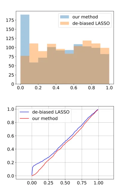
2.3 Adversarial perturbation generated using the fast gradient sign method [GSS14]133 3.1 Comparison of our de-biased estimator and oracle de-biased LASSO estimator 135 3.2 Comparison of our high dimensional linear regression point estimate with the vanilla LASSO estimate . . . 136

(15)

List of Algorithms

1 Unregularized M-estimation statistical inference . . . 28

2 SVRG based statistical inference algorithm in unregularized M-estimation. . 35

3 High dimensional linear regression statistical inference. . . 47

4 Computing the de-biased estimator (5.4) via SVRG . . . 48

5 Solving the high dimensional linear regression optimization objective (5.1) using proximal SVRG. . . 49

(16)

Chapter 1 Introduction

Statistical inference, such as hypothesis testing and calculating a confidence interval, is an important tool for accessing uncertainty in machine learning and statistical problems, both for estimation and prediction purposes [FHT01,EH16]. E.g., in unregularized linear regression and high-dimensional LASSO settings [vdGBRD14, JM15, TWH15], we are interested in computing coordinate-wise confidence intervals and p-values of a p-dimensional variable, in order to infer which coordinates are active or not [Was13]. Traditionally, the inverse Fisher information matrix [Edg08] contains the answer to such inference questions; however it requires storing and computing a p×pmatrix structure, often prohibitive for large-scale applications [TRVB06]. Alternatively, the Bootstrap [Efr82, ET94] method is a popular statistical inference algorithm, where we solve an optimization problem per dataset replicate, but can be expensive for large data sets [KTSJ14].

Stochastic gradient methods, such as stochastic gradient descent (SGD) [RM85,

Bub15a, Bot10], have been recently been successfully applied to point estimation in large scale machine learning problems. For example, in deep learning [GBC16], stochastic gradient methods such as SGD and Adam [KB14] are widely used to train neural nets.

In this context, we follow a different path: we show that inference can also be accomplished by directly using stochastic gradient methods, such as SGD, both for point estimates and inference. While optimization is mostly used for point estimates, recently it This chapter also appears in [LKLC18,LLKC18]. It was written by Tianyang Li, and edited by Anastasios Kyrillidis and Constantine Caramanis.

(17)

is also used as a means for statistical inference in large scale machine learning [LKLC18,

LLKC18, CLTZ16, SZ18, FXY17].

In Chapter 3, we present a statistical inference procedure using SGD with fixed step size [LLKC18]. It is well-established that fixed step-size SGD is by and large the dominant method used for large scale data analysis. We prove, and also demonstrate empirically, that

the average of SGD sequences, obtained by empirical risk minimization (ERM), can also be used for statistical inference. Unlike the Bootstrap, our approach does not require creating many large-size subsamples from the data, neither re-running SGD from scratch for each of these subsamples. Our method only uses first order information from gradient computations, and does not require any second order information. Both of these are important for large scale problems, where re-sampling many times, or computing Hessians, may be computationally prohibitive.

In Chapter 4, we present a framework for approximate Newton-based statistical inference using only stochastic gradients [LKLC18]. This is enabled by the fact that we only need to compute Hessian-vector products; in math, this can be approximated using

∇2_f₍_θ₎_v _≈ ∇f(θ+δv)−∇f(θ)

δ , wheref is the objective function, and∇f,∇

2_f _{denote the gradient}

and Hessian of f. Our method can be interpreted as a generalization of stochastic variance reduced gradient (SVRG) [JZ13] in optimization [JZ13] (Chapter 7); further, it is related to other stochastic Newton methods (e.g. [ABH17]) whenδ →0.

As an extension of the approximate Newton-based statistical inference procedure using stochastic gradients, in Chapter 5we present a novel statistical inference procedure for high dimensional linear regression using stochastic gradients, where the number of features is much larger than the number of samples. The intuition behind our algorithm is that each proximal Newton descent step [LSS14] can be solved using proximal SVRG [XZ14].

In Chapter6, we present a novel stochastic gradient framework for time series analysis, which correctly captures dependence relationships in a time series dataset. Unlike vanilla

(18)

SGD where we sample indices uniformly over the entire dataset, we sample contiguous blocks of indices, where the data-dependent block length is the lag. This enables our stochastic gradient procedure to compute a covariance estimate similar to the Driscoll-Kraay method [DK98, Hoe07]. The sampling scheme in our procedure is similar to that of moving block bootstrap [Lah13], and similar sampling schemes in conformal prediction for time series analysis [BHV14], which also use contiguous blocks chosen from the dataset.

1.1 Related work

1.1.1 Connection with Bootstrap methods

The classical approach for statistical inference is to use the bootstrap [ET94, ST12]. Bootstrap samples are generated by replicating the entire data set by resampling, and then solving the optimization problem on each generated set of the data. We identify our algorithm and its analysis as an alternative to bootstrap methods. Our analysis is also specific to SGD, and thus sheds light on the statistical properties of this very widely used algorithm.

In bootstrap, given a dataset with n samples, each time we resample n times with replacement from the dataset, and compute an estimate (replicate) on this resampled dataset. We then perform statistical inference, such as hypothesis testing or computing confidence intervals, using the empirical distribution of bootstrap replicates.

In jackknife, we generaten datasets, where each dataset hasn−1 elements, by leaving out one element each time. We then use the variance of jackknife replicates in asymptotic normality to perform statistical inference, such as hypothesis testing or computing confidence intervals.

(19)

1.1.2 Other stochastic gradient methods for frequentist inference

This work provides a general, flexible framework forsimultaneous point estimation and statistical inference, and improves upon previous methods, based on averaged stochastic gradient descent [LLKC18, CLTZ16].

Compared to [CLTZ16] (and similar works [SZ18, FXY17] using SGD with decreasing step size), our method does not need to increase the lengths of “segments” (inner loops) to reduce correlations between different “replicates”. Even in that case, if we use T replicates and increasing “segment” length (number of inner loops ist1−dodo·L) with a total ofO(T

1 1−do·L)

stochastic gradient steps, [CLTZ16] guarantees O(L−1−2do +T− 1 2+Tmax{ 1 2− do 4(1−do),0}− 1 2·L−do4 + Tmax{2(11−−2dodo),0}− 1

2 ·L1−22do) , whereas our method guarantees O(T−

do

2 ). Further, [CLTZ16] is

inconsistent, whereas our scheme guarantees consistency of computing the statistical error covariance.

Chapter 3[LLKC18] uses fixed step size SGD for statistical inference, and discards iterates between different “segments” to reduce correlation, whereas we do not discard any iterates in our computations. Although [LLKC18] states empirically constant step SGD performs well in statistical inference, it has been empirically shown [DDB17] that averaging consecutive iterates in constant step SGD does not guarantee convergence to the optimal – the average will be “wobbling” around the optimal, whereas decreasing step size stochastic approximation methods ([PJ92, Rup88] and our work) will converge to the optimal, and averaging consecutive iterates guarantees “fast” rates.

1.1.3 Stochastic gradient methods for Bayesian inference

First and second order iterative optimization algorithms –including SGD, gradient descent, and variants– naturally define a Markov chain. Based on this principle, most related to this work is the case of stochastic gradient Langevin dynamics (SGLD) for Bayesian inference – namely, for sampling from the posterior distributions – using a variant of SGD

(20)

[WT11,BEL15,MHB16,MHB17]. We note that, here as well, the vast majority of the results rely on using a decreasing step size. Very recently, [MHB17] uses a heuristic approximation for Bayesian inference, and provides results for fixed step size.

Our problem is different in important ways from the Bayesian inference problem. In such parameter estimation problems, the covariance of the estimator only depends on the gradient of the likelihood function. This is not the case, however, in general frequentist

M-estimation problems (e.g., linear regression). In these cases, the covariance of the estimator depends both on the gradient and Hessian of the empirical risk function. For this reason, without second order information, SGLD methods are poorly suited for general M-estimation problems in frequentist inference. In contrast, our method exploits properties of averaged SGD, and computes the estimator’s covariance without second order information. Another key difference between our methods and SGLD methods, is that we use averages of consecutive iterates, whereas SGLD does not use averaging.

SGLD can be viewed as a discretization of the following stochastic differential equation ind-dimensional space

dz=f(z)dt+p2D(z)dW(t),

where f(z) is a deterministic drift, W(t) is a standard Brownian motion process, and D(z) is a positive semidefinite diffusion matrix. [MCF15] shows that its stationary distribution exp(₋H(z)), when f(z) =−[D(z) +Q(z)]∇H(z) + Γ(z), Γi(z) = d X j=1 ∂ ∂zj [Dij(z) +Qij(z)],

(21)

1.1.4 Related optimization algorithms

1.1.4.1 Connection with stochastic approximation methods

It has been long observed in stochastic approximation that under certain conditions, SGD displays asymptotic normality for both the setting ofdecreasing step size, e.g., [LPW12,

PJ92], and more recently, [TA14,CLTZ16]; and also forfixed step size, e.g., [BPM90], Chapter 4. All of these results, however, provide their guarantees with the requirement that the stochastic approximation iterate converges to the optimum. For decreasing step size, this is not an overly burdensome assumption, since with mild assumptions it can be shown directly. As far as we know, however, it is not clear if this holds in the fixed step size regime. To side-step this issue, [BPM90] provides results only when the (constant) step-size approaches 0 (see Section 4.4 and 4.6, and in particular Theorem 7 in [BPM90]). Similarly, while [KY03] has asymptotic results on the average of consecutive stochastic approximation iterates with constant step size, it assumes convergence of iterates (assumption A1.7 in Ch. 10) – an assumption we are unable to justify in even simple settings.

Beyond the critical difference in the assumptions, the majority of the “classical” subject matter seeks to prove asymptotic results about different flavors of SGD, but does not properly consider its use for inference. Key exceptions are the recent work in [TA14] and [CLTZ16], which follow up on [PJ92]. Both of these rely on decreasing step size, for reasons mentioned above. The work in [CLTZ16] uses SGD with decreasing step size for estimating an M-estimate’s covariance. Work in [TA14] studies implicit SGD with decreasing step size and proves results similar to [PJ92], however it does not use SGD to compute confidence intervals.

Overall, to the best of our knowledge, there are no prior results establishing asymptotic normality for SGD with fixed step size for general M-estimation problems (that do not rely on overly restrictive assumptions, as discussed).

(22)

1.1.4.2 Connections to stochastic Newton methods

Our method is similar to stochastic Newton methods (e.g. [ABH17]); however, our method only uses first-order information to approximate a Hessian vector product (∇2_f₍_θ₎_v _≈ ∇f(θ+δv)−∇f(θ)

δ ). Algorithm 1’s outer loops are similar to stochastic natural gradient descent [Ama98]. Also, we demonstrate an intuitive view of SVRG [JZ13] as a special case of approximate stochastic Newton steps using first order information (Chapter7). 1.1.5 Statistical inference in high dimensional linear regression

[CLTZ16]’s high dimensional inference algorithm is based on [ANW12], and only guarantees that optimization error is at the same scale as the statistical error. However, proper de-biasing of the LASSO estimator requires the optimization error to be much less than the statistical error, otherwise the optimization error introduces additional bias that de-biasing cannot handle. Our optimization objective is strongly convex with high probability: this permits the use of linearly convergent proximal algorithms [XZ14, LSS14] towards the optimum, which guarantees the optimization error to be much smaller than the statistical error.

Our method of de-biasing the LASSO Chapter 5 is similar to [ZZ14, vdGBRD14,

JM14, JM15]. Our method uses a new `1 regularized objective for high dimensional linear

regression, and we have different de-biasing terms, because we also need to de-bias the covariance estimation. In Algorithm 3, our covariance estimate is similar to the classic

sandwich estimator [Hub67, Whi80]. Previous methods require O(p2_{) space which unsuitable}

for large scale problems, whereas our method only requires O(p) space. Similar to our `1

-norm regularized objective, [YLR14,JD11] shows similar point estimate statistical guarantees for related estimators; however there are no confidence interval results. Further, although [YLR14] is an elementary estimator in closed form, it still requires computing the inverse of the thresholded covariance, which is challenging in high dimensions, and may not computationally

(23)

outperform optimization approaches.

Finally, for feature selection, we do not assume that absolute values of the true parameter’s non-zero entries are lower bounded. [FGLS18,Wai09, BvdG11].

Time series analysis. Our approach of sampling contiguous blocks of indices to compute stochastic gradients for statistical inference in time series analysis is similar to resampling procedures inmoving block orcircularbootstrap [Car86,Kun89,B¨uh02,DH97,ET94,Lah13,

PR92, PR94,KL12], and conformal prediction[BHV14,SV08,VGS05]. Also, our procedure is similar to Driscoll-Kraay standard errors [DK98, KD99, Hoe07], but does not waste computational resources to explicitly store entire matrices, and is suited for large scale time series analysis.

(24)

Chapter 2 Statistical inference in

M

-estimation

Here, we give a brief overview of statistical inference in unregularized M-estimation. Consider the problem of estimating a set of parameters θ? _∈

Rp using n samples {Xi}n_i₌₁, drawn from some distribution P on the sample space X. In frequentist inference, we are interested in estimating the minimizer θ? _{of the population risk:}

θ? = argmin θ∈_Rp EP [f(θ;X)] = argmin θ∈_Rp Z x f(θ;x) dP(x), (2.1) where we assume thatf(_·;x) : _Rp _→

Ris real-valued and convex; further, we will useE≡EP, unless otherwise stated. In practice, the distribution P is unknown. We thus estimate θ? _by solving an empirical risk minimization (ERM) problem, where we use the estimate θb:

b θ = argmin θ∈Rp 1 n n X i=1 f(θ;Xi). (2.2)

Statistical inference consists of techniques for obtaining information beyond point estimates θb, such as confidence intervals. These can be performed if there is an asymptotic limiting distribution associated with θb[Was13]. Indeed, under standard and well-understood regularity conditions, the solution to M-estimation problems satisfies asymptotic normality. That is, the distribution √n(θb−θ?) converges weakly to a normal distribution:

√ n(θb−θ?)−→N(0, H? −1 G?H?−1), (2.3) where H? =E[∇2f(θ?;X)],

This chapter also appears in [LKLC18,LLKC18]. It was written by Tianyang Li, and edited by Anastasios Kyrillidis and Constantine Caramanis.

(25)

and

G? =E[∇f(θ?;X)· ∇f(θ?;X)>];

see also Theorem 5.21 in [vdV00]. We can therefore use this result, as long as we have a good estimate of the covariance matrix: H?−1

G?_H?−1

. The central goal of this paper is obtaining accurate estimates for H?−1_G?_H?−1_.

A naive way to estimate H?−1_G?_H?−1 _{is through the empirical estimator}

b H−1 b GHb−1 where: b H = 1 n n X i=1 ∇2 f(θb;Xi) and b G= 1 n n X i=1 ∇f(bθ;Xi)∇f(θb;Xi)>. (2.4) Beyond calculating1 b

H andGb, this computation requires an inversion of Hb and matrix-matrix multiplications in order to compute Hb−1GbHb−1—a key computational bottleneck in high dimensions. Instead, our method uses SGD to directly estimate Hb−1GbHb−1.

1_{In the case of maximum likelihood estimation, we have}_H?₌_G?_{—which is called Fisher information.}

Thus, the covariance of interest isH?−1₌_G?−1_{. This can be estimated either using} b H or G.b

(26)

Chapter 3 Statistical inference using SGD

Here, we describe our procedure for statistical inference in unregularizedM-estimation using SGD.

3.1 Statistical inference using SGD

Consider the optimization problem in (2.2). For instance, in maximum likelihood estimation (MLE), f(θ;Xi) is a negative log-likelihood function. For simplicity of notation, we use fi(θ) and f(θ) forf(θ;Xi) and 1

n Pn

i=1f(θ;Xi), respectively, for the rest of the paper.

The SGD algorithm with a fixed step sizeη, is given by the iteration

θt+1 =θt−ηgs(θt), (3.1)

where gs(_·) is an unbiased estimator of the gradient, i.e., E[gs(θ) | θ] =∇f(θ), where the

expectation is w.r.t. the stochasticity in the gs(·) calculation. A classical example of an unbiased estimator of the gradient is gs(_·)_{≡ ∇}fi(_·), where i is a uniformly random index over the samples Xi.

Our inference procedure uses the average of t consecutive SGD iterations. In particular, the algorithm proceeds as follows: Given a sequence of SGD iterates, we use the first SGD This chapter also appears in [LLKC18]. The theoretical analysis was written by Tianyang Li, and the experiments were conducted in collaboration with Liu Liu. It was edited by Anastasios Kyrillidis and Constantine Caramanis.

(27)

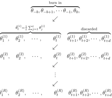
burn in z }| { θ−b, θ−b+1,· · ·θ−1, θ0, . ¯ θ(_ti)=1 t Pt j=1θ (i) j z }| { θ(1)₁ , θ₂(1), _{· · ·} , θ(1)t discarded z }| { θ_t(1)₊₁, θ(1)_t₊₂,_{· · ·} , θ_t(1)₊_d . θ₁(2), θ(2)₂ , _{· · ·} , θt(2) θ (2) t+1, θ (2) t+2,· · · , θ (2) t+d . ... . θ(₁R), θ₂(R), _{· · ·} , θt(R) θ (R) t+1, θ (R) t+2,· · · , θ (R) t+d

Figure 3.1: Our SGD inference procedure

iterates θ−b, θ−b+1, . . . , θ0 as a burn in period; we discard these iterates. Next, for each

“segment” oft+diterates, we use the firstt iterates to compute ¯θt(i) = 1t Pt

j=1θ (i)

j and discard the lastd iterates, where i indicates the i-th segment. This procedure is illustrated in Figure

3.1. As the final empirical minimumθb, we use in practice θb≈ _R1 PR

i=1θ¯ (i)

t [Bub15b]. Some practical aspects of our scheme are discussed below.

Step size η selection and length t: Theorem 1 below is consistent only for SGD with fixed step size that depends on the number of samples taken. Our experiments, however, demonstrate that choosing a constant (large)ηgives equally accurate results with significantly reduced running time. We conjecture that a better understanding of t’s and η’s influence requires stronger bounds for SGD with constant step size. Heuristically, calibration methods for parameter tuning in subsampling methods ([ET94], Ch.18; [PRW12], Ch. 9) could be used for hyper-parameter tuning in our SGD procedure. We leave the problem of finding maximal (provable) learning rates for future work.

(28)

Discarded length d: Based on the analysis of mean estimation in the appendix, if we discard d SGD iterates in every segment, the correlation between consecutiveθ(i) _and _θ(i+1)

is of the order ofC1e−C2ηd, where C1 andC2 are data dependent constants. This can be used

as a rule of thumb to reduce correlation between samples from our SGD inference procedure.

Burn-in period b: The purpose of the burn-in period b, is to ensure that samples are generated when SGD iterates are sufficiently close to the optimum. This can be determined using heuristics for SGD convergence diagnostics. Another approach is to use other methods (e.g., SVRG [JZ13]) to find the optimum, and use a relatively small b for SGD to reach

stationarity, similar to Markov Chain Monte Carlo burn-in.

Statistical inference using θ¯t(i) and θ:b Similar to ensemble learning [OM99], we use

i= 1,2, . . . , R estimators for statistical inference:

θ(i)₌ b θ+ r Ks·t n ¯ θ(_ti)₋θb . (3.2)

Here, Ks is a scaling factor that depends on how the stochastic gradient gs is computed. We show examples of Ks for mini batch SGD in linear regression and logistic regression in the corresponding sections. Similar to other resampling methods such as bootstrap and subsampling, we use quantiles or variance of θ(1)_{, θ}(2)_{, . . . , θ}(R) _{for statistical inference.}

3.1.1 Theoretical guarantees

Next, we provide the main theorem of our paper. Essentially, this provides conditions under which our algorithm is guaranteed to succeed, and hence has inference capabilities. Theorem 1. For a differentiable convex function f(θ) = 1

n Pn

i=1fi(θ), with gradient ∇f(θ),

let θb∈Rp be its minimizer, according to (2.2), and denote its Hessian at θbby H :=∇2f(θb) =

1 n· Pn i=1∇ 2_f_i( b

θ). Assume that_∀θ ∈Rp, f satisfies:

(29)

(F2) Lipschitz gradient continuity: k∇f(θ)k2 ≤Lkθ−θbk₂, for constant L >0,

(F3) Bounded Taylor remainder: k∇f(θ)−H(θ−bθ)k2 ≤Ekθ−θbk2₂, for constant E >0,

(F4) Bounded Hessian spectrum at bθ: 0< λ_L ≤λi(H)≤λ_U <∞, ∀i.

Furthermore, let gs(θ) be a stochastic gradient of f, satisfying: (G1) E[gs(θ)|θ] =∇f(θ), (G2) E[kgs(θ)k22 |θ]≤Akθ−θbk2₂+B, (G3) E[kgs(θ)k42 |θ]≤Ckθ−θbk4₂ +D, (G4) E gs(θ)gs(θ)>_|_θ −G 2 ≤A1kθ−θbk2+A2kθ−θbk 2 2+A3kθ−bθk3₂+A₄kθ−θbk4₂,

where G=E[gs(bθ)gs(θb)>|θb] and, for positive, data dependent constants A, B, C, D, A_i, for

i= 1, . . . ,4.

Assume that _kθ1−θbk₂2 =O(η); then for sufficiently small step sizeη >0, the average

SGD sequence, θ¯t, satisfies: tE[(¯θt−θb)(¯θt−θb) > ]−H−1GH−1 2 .√η+q1 tη +tη2. (3.3)

We provide the full proof in the appendix, and also we give precise (data-dependent) formulas for the above constants. For ease of exposition, we leave them as constants in the expressions above. Further, in the next section, we relate a continuous approximation of SGD to Ornstein-Uhlenbeck process [RM51] to give an intuitive explanation of our results.

Discussion. For linear regression, assumptions (F1), (F2), (F3), and (F4) are satisfied

(30)

replacement, assumptions (G1), (G2), (G3), and (G4) are satisfied. Linear regression’s result

is presented in Corollary 2 in the appendix.

For logistic regression, assumption (F1) is not satisfied because the empirical risk

function in this case is strictly but not strongly convex. Thus, we cannot apply Theorem 1

directly. Instead, we consider the use of SGD on the square of the empirical risk function plus a constant; see eq. (3.7) below. When the empirical risk function is not degenerate, (3.7) satisfies assumptions (F1), (F2), (F3), and (F4). We cannot directly use vanilla SGD

to minimize (3.7), instead we describe a modified SGD procedure for minimizing (3.7) in Section 3.1.3, which satisfies assumptions (G1), (G2), (G3), and (G4). We believe that this

result is of interest by its own. We present the result specialized for logistic regression in Corollary 1.

Note that Theorem 1proves consistency for SGD with fixed step size, requiring η→0 when t→ ∞. However, we empirically observe in our experiments that a sufficiently large

constant η gives better results. We conjecture that the average of consecutive iterates in SGD with larger constant step size converges to the optimum and we consider it for future work. 3.1.2 Intuitive interpretation via the Ornstein-Uhlenbeck process

approxima-tion

Here, we describe a continuous approximation of the discrete SGD process and relate it to the Ornstein-Uhlenbeck process [RM51], to give an intuitive explanation of our results. In particular, under regularity conditions, the stochastic process ∆t=θt−θbasymptotically converges to an Ornstein-Uhlenbeck process ∆(t), [KH81, Pfl86, BPM90, KY03, MHB16] that satisfies:

d∆(T) = −H∆(T) dT +√ηG12 dB(T), (3.4)

(31)

√ t(¯θt−θb) = √1 t t X i=1 (θi−θb) = 1 η√t t X i=1 (θi−θb)η≈ 1 η√t Z tη 0 ∆(T) dT, (3.5)

where we use the approximation that η _≈ dT. By rearranging terms in (3.4) and multiplying both sides by H−1_{, we can rewrite the stochastic differential equation (}_3.4_{) as}

∆(T) dT =−H−1_d∆(_T_{) +}√_ηH−1_G1₂ _d_B₍_T_{). Thus, we have} Z tη 0 ∆(T) dT = −H−1_(∆(_tη₎ −∆(0)) +√ηH−1_G1₂_B₍_tη₎_. _(3.6)

After plugging (3.6) into (3.5) we have

√ tθ¯t−θb ≈ − 1 η√tH −1_(∆(_tη₎ −∆(0)) +_√1 tηH −1_G1₂_B₍_tη₎_.

When ∆(0) = 0, the variance Var

−1_/_η√_t_·_H−1_(∆(_tη₎₋_∆(0))

= O(1_/_tη_{). Since} 1_/√_tη_·

H−1_G1₂_B₍_tη₎_∼_N₍₀_{, H}−1_GH−1_{), when} _η_→_{0 and} _ηt_{→ ∞}_{, we conclude that}

√

t(¯θt−bθ)∼N(0, H−1GH−1). 3.1.3 Logistic regression

We next apply our method to logistic regression. We havensamples (X1, y1),(X2, y2), . . .(Xn, yn) where Xi ∈Rp consists of features and yi ∈ {+1,−1} is the label. We estimate θ of a linear

classifier sign(θT_X_{) by:}

b θ = argmin θ∈Rp 1 n n X i=1 log 1 + exp(−yiθ>Xi) .

(32)

We cannot apply Theorem1directly because the empirical logistic risk is not strongly convex; it does not satisfy assumption (F1). Instead, we consider the convex function

f(θ) = 1 2 c+ 1 n n X i=1 log1 + exp(−yiθ>Xi) !2 , where c >0 (e.g.,c= 1). (3.7) The gradient of f(θ) is a product of two terms

∇f(θ) = c+ 1 n n X i=1 log1 + exp(−yiθ>Xi) ! | {z } Ψ × ∇ _n1 n X i=1 log1 + exp(₋yiθ>Xi) ! | {z } Υ .

Therefore, we can compute gs = ΨsΥs, using two independent random variables satisfying

E[Ψs|θ] = Ψ andE[Υs |θ] = Υ. For Υs, we have Υs= S1Υ

P i∈IΥ

t ∇log(1 + exp(−yiθ

>_X_i)),

where IΥ

t areSΥ indices sampled from [n] uniformly at random with replacement. For Ψs, we

have Ψs=c+ 1 SΨ P i∈IΨ t log(1 + exp(−yiθ >_X_{i)), where} _IΨ

t are SΨ indices uniformly sampled

from [n] with or without replacement. Given the above, we have ∇f(θ)>₍_θ₋

b

θ)≥αkθ−θbk2₂ for some constantα by the generalized self-concordance of logistic regression [Bac10,Bac14], and therefore the assumptions are now satisfied.

For convenience, we write k(θ) = 1

n Pn

i=1ki(θ) where ki(θ) = log(1 + exp(−yiθ>Xi)). Thus f(θ) = (k(θ) +c)2_,

E[Ψs|θ] =k(θ) +c, andE[Υs |θ] =∇k(θ).

Corollary 1. Assume _kθ1−θbk2₂ = O(η); also S_Ψ =O(1), S_Υ =O(1) are bounded. Then, we

have tE h (¯θt−θb)(¯θ_t−θb)> i −H−1_GH−1 2. √_η₊q 1 tη +tη2, where H = _∇2_f₍ b θ) = (c+k(θb))∇2k(θb). Here, G = 1 SΥKG(θb) 1 n Pn i=1∇ki(bθ)ki(θb) > _with

(33)

−1.00 −0.75 −0.50 −0.25 0.00 0.25 0.50 0.75 1.00 0.0 0.5 1.0 1.5 2.0 N(0,1/n) θSGD−¯θSGD θbootstrap−¯θbootstrap (a) Normal. 0.8 1.0 1.2 1.4 1.6 0 1 2 3 4 SGD bootstrap (b) Exponential. 0.8 1.0 1.2 1.4 0 1 2 3 4 5 SGD_bootstrap (c) Poisson. Figure 3.2: Estimation in univariate models.

with replacement: KG(θ) = _S1 Ψ( 1 n Pn i=1(c+ki(θ))2) + SΨ−1 SΨ (c+k(θ)) 2 _, no replacement: KG(θ) = 1−SΨ−1 n−1 SΨ ( 1 n Pn i=1(c+ki(θ))2) +SΨ_S_Ψ−1_nn−1(c+k(θ))2.

Quantities other than t and η are data dependent constants.

As with the results above, in the appendix we give data-dependent expressions for the constants. Simulations suggest that the termtη2_{in our bound is an artifact of our analysis.}

Be-cause in logistic regression the estimate’s covariance is (∇

2_k_(b_θ₎₎−1 n Pn i=1∇ki(θb)∇ki(bθ)> n ∇ 2_k₍ b θ) −1 , we set the scaling factor Ks = (c+k(

b

θ))2

KG(θb) in (3.2) for statistical inference. Note that Ks≈1 for

sufficiently large SΨ.

η t= 100 t= 500 t= 2500

0.1 (0.957, 4.41) (0.955, 4.51) (0.960, 4.53)

0.02 (0.869, 3.30) (0.923, 3.77) (0.918, 3.87)

0.004 (0.634, 2.01) (0.862, 3.20) (0.916, 3.70)

(a) Bootstrap (0.941, 4.14), normal approximation (0.928, 3.87)

η t= 100 t= 500 t= 2500

0.1 (0.949, 4.74) (0.962, 4.91) (0.963, 4.94)

0.02 (0.845, 3.37) (0.916, 4.01) (0.927, 4.17)

0.004 (0.616, 2.00) (0.832, 3.30) (0.897, 3.93)

(b) Bootstrap (0.938, 4.47), normal approximation (0.925, 4.18)

(34)

η t= 100 t= 500 t= 2500 0.1 (0.872, 0.204) (0.937, 0.249) (0.939, 0.258) 0.02 (0.610, 0.112) (0.871, 0.196) (0.926, 0.237) 0.004 (0.312, 0.051) (0.596, 0.111) (0.86, 0.194)

(a) Bootstrap (0.932, 0.253), normal approximation (0.957, 0.264)

η t= 100 t= 500 t= 2500

0.1 (0.859, 0.206) (0.931, 0.255) (0.947, 0.266) 0.02 (0.600, 0.112) (0.847, 0.197) (0.931, 0.244) 0.004 (0.302, 0.051) (0.583, 0.111) (0.851, 0.195) (b) Bootstrap (0.932, 0.245), normal approximation (0.954, 0.256)

Table 3.2: Logistic regression. Left: Experiment 1, Right: Experiment 2.

3.2 Experiments

3.2.1 Synthetic data

The coverage probability is defined as 1

p Pp

i=1P[θ

?

i ∈Cˆi] whereθ? = argminθE[f(θ, X)]∈Rp, and ˆCi is the estimated confidence interval for the ith coordinate. The average confidence interval width is defined as 1

p Pp

i=1( ˆC

u

i − Cˆil) where [ ˆCil,Cˆiu] is the estimated confidence interval for theith _{coordinate. In our experiments, coverage probability and average}

confi-dence interval width are estimated through simulation. We use the empirical quantile of our SGD inference procedure and bootstrap to compute the 95% confidence intervals for each coordinate of the parameter. For results given as a pair (α, β), it usually indicates (coverage probability, confidence interval length).

3.2.1.1 Univariate models

In Figure 3.2, we compare our SGD inference procedure with (i) Bootstrap and (ii) normal approximation with inverse Fisher information in univariate models. We observe that our method and Bootstrap have similar statistical properties. Figure 1.1 in the appendix shows Q-Q plots of samples from our SGD inference procedure.

Normal distribution mean estimation: Figure 3.2a compares 500 samples from SGD inference procedure and Bootstrap versus the distribution N(0,1/n), using n = 20 i.i.d. samples from N(0,1). We used mini batch SGD described in Section3.4. For the parameters, we usedη = 0.8, t= 5,d= 10,b = 20, and mini batch size of 2. Our SGD inference procedure

(35)

gives (0.916 , 0.806), Bootstrap gives (0.926 , 0.841), and normal approximation gives (0.922 , 0.851).

Exponential distribution parameter estimation: Figure3.2bcompares 500 samples from inference procedure and Bootstrap, usingn = 100 samples from an exponential distribution with PDF λe−λx _where _λ _{= 1. We used SGD for MLE with mini batch sampled with} replacement. For the parameters, we used η= 0.1, t= 100, d= 5, b = 100, and mini batch size of 5. Our SGD inference procedure gives (0.922, 0.364), Bootstrap gives (0.942 , 0.392), and normal approximation gives (0.922, 0.393).

Poisson distribution parameter estimation: Figure 3.2c compares 500 samples from inference procedure and Bootstrap, using n= 100 samples from a Poisson distribution with PDFλx_e−λx_where_λ _{= 1. We used SGD for MLE with mini batch sampled with replacement.} For the parameters, we used η= 0.1, t= 100,d = 5, b= 100, and mini batch size of 5. Our SGD inference procedure gives (0.942 , 0.364), Bootstrap gives (0.946 , 0.386), and normal approximation gives (0.960 , 0.393).

3.2.1.2 Multivariate models

In these experiments, we set d= 100, used mini-batch size of 4, and used 200 SGD samples. In all cases, we compared with Bootstrap using 200 replicates. We computed the coverage probabilities using 500 simulations. Also, we denote 1p =

1 1 . . . 1>

∈ Rp.

Additional simulations comparing covariance matrix computed with different methods are given in Sec. 1.1.1.1.

Linear regression: Experiment 1: Results for the case where X ∼ N(0, I) ∈ R10, Y = w∗T_X ₊_, _w∗ _{= 1p}_/√_p_{, and}

∼ N(0, σ2 _{= 10}2_{) with} _n _{= 100 samples is given in}

Table 3.1a. Bootstrap gives (0.941, 4.14), and confidence intervals computed using the error covariance and normal approximation gives (0.928, 3.87). Experiment 2: Results for the case

(36)

whereX _∼N(0,Σ)_∈R10, Σij = 0.3|i−j|,Y =w∗TX+,w∗ = 1p/√p, and∼N(0, σ2 = 102)

with n= 100 samples is given in Table 3.1b. Bootstrap gives (0.938, 4.47), and confidence intervals computed using the error covariance and normal approximation gives (0.925, 4.18).

Logistic regression: Here we show results for logistic regression trained using vanilla SGD with mini batch sampled with replacement. Results for modified SGD (Sec. 3.1.3) are given in Sec. 1.1.1.1. Experiment 1: Results for the case whereP[Y = +1] =P[Y =−1] = 1/2, X _|Y _∼N(0.01Y1p/√p, I)_∈R10 withn = 1000 samples is given in Table 3.2a. Bootstrap

gives (0.932, 0.245), and confidence intervals computed using inverse Fisher matrix as the error covariance and normal approximation gives (0.954, 0.256). Experiment 2: Results for the case where P[Y = +1] = P[Y = −1] = 1/2, X | Y ∼ N(0.01Y1p/√p,Σ) ∈ R10,

Σij = 0.2|i−j| _with _n_{= 1000 samples is given in Table} _3.2b_{. Bootstrap gives (0.932, 0.253),}

and confidence intervals computed using inverse Fisher matrix as the error covariance and normal approximation gives (0.957, 0.264).

3.2.2 Real data

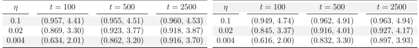
Here, we compare covariance matrices computed using our SGD inference procedure, bootstrap, and inverse Fisher information matrix on the LIBSVM Splice data set, and we observe that they have similar statistical properties.

3.2.2.1 Splice data set

The Splice data set 1 _{contains 60 distinct features with 1000 data samples. This is a}

classification problem between two classes of splice junctions in a DNA sequence. We use a logistic regression model trained using vanilla SGD.

In Figure3.3, we compare the covariance matrix computed using our SGD inference

1

(37)

procedure and bootstrap n = 1000 samples. We used 10000 samples from both bootstrap and our SGD inference procedure with t = 500,d= 100, η= 0.2, and mini batch size of 6.

0 10 20 30 40 50 60 0 10 20 30 40 50 60 0.02 0.01 0.00 0.01 0.02 (a) Bootstrap 0 10 20 30 40 50 60 0 10 20 30 40 50 60 0.02 0.01 0.00 0.01 0.02 (b) SGD inference covariance Figure 3.3: Splice data set

0 5 10 15 20 25 0 5 10 15 20 25

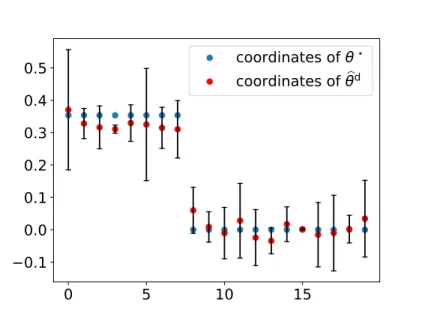
(a) Original “0”: logit -46.3, CI (-64.2, -27.9) 0 5 10 15 20 25 0 5 10 15 20 25 (b) Adversarial “0”: logit 16.5, CI (-10.9, 30.5) Figure 3.4: MNIST

(38)

3.2.2.2 MNIST

Here, we train a binary logistic regression classifier to classify 0/1 using a noisy MNIST data set, and demonstrate that adversarial examples produced by gradient attack [GSS14] (perturbing an image in the direction of loss function’s gradient with respect to data) can be detected using prediction intervals. We flatten each 28×28 image into a 784 dimensional vector, and train a linear classifier using pixel values as features. To add noise to each image, where each original pixel is either 0 or 1, we randomly changed 70% pixels to random numbers uniformly on [0,0.9]. Next we train the classifier on the noisy MNIST data set, and generate adversarial examples using this noisy MNIST data set. Figure3.4 shows each image’s logit value (logP[1|image]

P[0|image]) and its 95% confidence interval (CI) computed using quantiles from our

SGD inference procedure.

3.2.3 Discussion

In our experiments, we observed that using a larger step size η produces accurate results with significantly accelerated convergence time. This might imply that the η term in Theorem 1’s bound is an artifact of our analysis. Indeed, although Theorem1 only applies to SGD with fixed step size, where ηt_{→ ∞}and η2_t_→_{0 imply that the step size should be}

smaller when the number of consecutive iterates used for the average is larger, our experiments suggest that we can use a (data dependent) constant step sizeη and only requireηt_{→ ∞}.

In the experiments, our SGD inference procedure uses (t+d)·S·p operations to produce a sample, and Newton method uses n _·(matrix inversion complexity = Ω(p2₎₎_·

(number of Newton iterations t) operations to produce a sample. The experiments therefore suggest that our SGD inference procedure produces results similar to Bootstrap while using far fewer operations.

(39)

3.3 Linear Regression

In linear regression, the empirical risk function satisfies:

f(θ) = 1 n n X i=1 1 2(θ > xi−yi)2,

where yi denotes the observations of the linear model and xi are the regressors. To find an estimate to θ?_{, one can use SGD with stochastic gradient give by:}

gs[θt] = 1

S

X i∈It

∇fi(θt),

where It are S indices uniformly sampled from [n] with replacement.

Next, we state a special case of Theorem 1. Because the Taylor remainder∇f(θ)−

H(θ₋θb) = 0, linear regression has a stronger result than general M-estimation problems. Corollary 2. Assume that _kθ1−bθk2₂ =O(η), we have

tE[(¯θt−bθ)(¯θt−θb) > ]₋H−1_GH−1 2 . √_η₊ 1 √ tη, where H = 1 n Pn i=1xix > i and G= 1 S 1 n Pn i=1(x > i θb−yi)2x_ix>_i .

We assume that S = O(1) is bounded, and quantities other than t and η are data dependent constants.

As with our main theorem, in the appendix we provide explicit data-dependent expressions for the constants in the result. Because in linear regression the estimate’s covariance is 1 n( 1 n Pn i=1xix > i ) −1₎₍1 n(x > i bθ−yi)(x_i>θb−yi)>)(1 n Pn i=1xix > i )

−1_{), we set the scaling}

(40)

3.4 Exact analysis of mean estimation

In this section, we give an exact analysis of our method in the least squares, mean estimation problem. For n i.i.d. samples X1, X2, . . . , Xn, the mean is estimated by solving

the following optimization problem ˆ θ = argmax θ∈_Rp 1 n n X i=1 1 2kXi−θk 2 2 = 1 n n X i=1 Xi.

In the case of mini-batch SGD, we sample S = O(1) indexes uniformly randomly with replacement from [n]; denote that index set as It. For convenience, we write Yt = _S1

P

i∈ItXi,

Then, in the tth _{mini batch SGD step, the update step is}

θt+1 =θt−η(θt−Yt) = (1−η)θt+ηYt, (3.8) which is the same as the exponential moving average. And we have

√ tθb_t=− 1 η√t(θt+1−θ1) + 1 √ t n X i=1 Yi. (3.9)

Assume that_kθ1−θbk2₂ =O(η), then from Chebyshev’s inequality − 1

η√t(θt+1−θ1)→0 almost surely when tη → ∞. By the central limit theorem, _√1

t Pn i=1Yi converges weakly toN(θ,b _S1Σ)ˆ with ˆΣ = 1 n Pn i=1(Xi−θb)(Xi−bθ) >_{. From (}_3.8_{), we have} kCov(θa, θb)k2 = O(η(1−η)|a−b|)

uniformly for all a, b, where the constant is data dependent. Thus, for our SGD inference procedure, we havekCov(θ(i)_{, θ}(j)₎_k

2 =O(η(1−η)d+t|i−j|). Our SGD inference procedure does

not generate samples that are independent conditioned on the data, whereas replicates are independent conditioned on the data in bootstrap, but this suggests that our SGD inference procedure can produce “almost independent” samples if we discard sufficient number of SGD iterates in each segment.

When estimating a mean using our SGD inference procedure where each mini batch is

(41)

Chapter 4 Approximate Newton-based statistical inference using

only stochastic gradients

In unregularized, low-dimensional M-estimation problems, we estimate a parameter of interest:

θ? = arg min

θ∈_RpEX∼P[`(X;θ)], where P(X) is the data distribution,

using empirical risk minimization(ERM) on n > p i.i.d. data points _{Xi}ni=1:

b θ = arg min θ∈_Rp 1 n n X i=1 `(Xi;θ).

Statistical inference, such as computing one-dimensional confidence intervals, gives us infor-mation beyond the point estimateθb, when bθ has an asymptotic limit distribution [Was13].

E.g., under regularity conditions, the M-estimator satisfies asymptotic normality [vdV98, Theorem 5.21]. I.e., √n(θb−θ?) weakly converges to a normal distribution:

√ nbθ−θ? →N 0, H?−1 G?_H?−1 , where H? ₌

EX∼P[∇2θ`(X;θ?)] and G? = EX∼P[∇θ`(X;θ?)∇θ`(X;θ?)>]. We can perform statistical inference when we have a good estimate of H?−1

G?_H?−1

. In this work, we use the This chapter also appears in [LKLC18]. The theoretical analysis was written by Tianyang Li, and the experiments were conducted in collaboration with Liu Liu. It was edited by Anastasios Kyrillidis and Constantine Caramanis.

(42)

plug-in covariance estimator Hb−1GbHb−1 for H?−1G?H?−1, where: b H = 1 n n X i=1 ∇2 θ`(Xi;θb), and Gb = _n1 n X i=1 ∇θ`(Xi;θb)∇θ`(Xi;θb)>.

Observe that, in the naive case of directly computing Gb and Hb−1, we require both high computational- and space-complexity. Here, instead, we utilize approximate stochastic Newton motions from first order information to compute the quantity Hb−1GbHb−1.

4.1 Statistical inference with approximate Newton steps using

only stochastic gradients

Based on the above, we are interested in solving the following p-dimensional optimiza-tion problem: b θ = arg min θ∈_Rpf(θ) := 1 n n X i=1 fi(θ), where fi(θ) = `(Xi;θ).

Notice thatHb−1GbHb−1 can be written as _n1 Pn i=1 b H−1_∇ θ`(Xi;θb) Hb−1∇_θ`(Xi;θb) > , which can be interpreted as the covariance of stochastic –inverse-Hessian conditioned– gradients at b

θ. Thus, the covariance of stochastic Newton steps can be used for statistical inference. Algorithm1approximates each stochastic Newton Hb−1∇θ`(Xi;bθ) step using only first order information. We start from θ0 which is sufficiently close to θb, which can be effectively achieved using SVRG [JZ13]; a description of the SVRG algorithm can be found in Chapter7. Lines 4, 5 compute a stochastic gradient whose covariance is used as part of statistical inference. Lines 6to 12use SGD to solve the Newton step,

min g∈Rp * 1 So X i∈Io ∇fi(θt), g + + 1 2ρt g,_∇2_f₍_θ_t)_g , (4.1)

which can be seen as a generalization of SVRG; this relationship is described in more detail in Chapter 7. In particular, these lines correspond to solving (4.1) using SGD by uniformly

(43)

Algorithm 1 Unregularized M-estimation statistical inference 1: Parameters: So, Si ∈Z+;ρ0, τ0 ∈R+; do, di ∈ 1₂,1

Initial state: θ0 ∈Rp

2: for t = 0 toT −1 do // approximate stochastic Newton descent 3: ρt ←ρ0(t+ 1)−do

4: Io ← uniformly sampleSo indices with replacement from [n] 5: g0_t ← −ρt 1 So P i∈Io∇fi(θt)

6: for j = 0 to L₋1do // solving (4.1) approximately using SGD 7: τj ←τ0(j+ 1)−di and δ

j

t ←O(ρ4tτj4)

8: Ii ← uniformly sampleSi indices without replacement from [n] 9: g_tj+1 ←g_tj−τj 1 Si P k∈Ii ∇fk(θt+δtjg j t)−∇fk(θt) δtj +τjg0t 10: end for

11: Use √So· _ρg¯t_t for statistical inference, where ¯gt = _L1₊₁ PL j=0g j t 12: θt+1 ←θt+gLt 13: end for

sampling a random fi, and approximating:

∇2 f(θ)g ≈ ∇f(θ+δtjg)−∇f(θ) δj_t =E h_∇ fi(θ+δjtg)−∇fi(θ) δ_tj |θ i . (4.2)

Finally, the outer loop (lines 2to 13) can be viewed as solving inverse Hessian conditioned stochastic gradient descent, similar to stochastic natural gradient descent [Ama98].

In terms of parameters, similar to [PJ92,Rup88], we use a decaying step size in Line 8 to control the error of approximating H−1_g_{. We set} _δj

t = O(ρ4tτj4) to control the error of approximating Hessian vector product using a finite difference of gradients, so that it is smaller than the error of approximating H−1_g _{using stochastic approximation. For similar}

reasons, we use a decaying step size in the outer loop to control the optimization error. The following theorem characterizes the behavior of Algorithm 1.

Theorem 2. For a twice continuously differentiable and convex function f(θ) = 1

n Pn

i=1fi(θ)

where each fi is also convex and twice continuously differentiable, assume f satisfies strong convexity: _∀θ1, θ2, f(θ2)≥f(θ1) +h∇f(θ1), θ2−θ1i+1₂αkθ2−θ1k22;

(44)

∀θ, each_k∇2_f_i(_θ₎_k

2 ≤βi, which implies that fi has Lipschitz gradient: ∀θ1, θ2, k∇fi(θ1)−

∇fi(θ2)k2 ≤βikθ1−θ2k2;

each _∇2fi is Lipschitz continuous: ∀θ1, θ2, k∇2fi(θ2)− ∇2fi(θ1)k2 ≤hikθ2−θ1k2.

In Algorithm 1, we assume that batch sizes So—in the outer loop—and Si—in the

inner loops—are O(1). The outer loop step size is ρt=ρ0·(t+ 1)−do, where do ∈ 1₂,1

is the decaying rate. (4.3)

In each outer loop, the inner loop step size is τj =τ0·(j + 1)−di, where di ∈ 1₂,1

is the decaying rate. (4.4)

The scaling constant for Hessian vector product approximation is δtj =δ0·ρ4t ·τ 4 j =o 1 (t+1)2₍_j₊₁₎2 . (4.5)

Then, for the outer iterate θt we have

E h kθt−θbk2₂ i .t−do_, _(4.6) and E h kθt−θbk4₂ i .t−2do_. _(4.7)

In each outer loop, after L steps of the inner loop, we have: E ¯ gt ρt −[∇ 2_f₍_θ_t)]−1_g0 t 2 2 |θt . L1 g_t0 2 2, (4.8)

and at each step of the inner loop, we have: E h gj_t+1−[∇2f(θt)]−1g_t0 4 2 |θt i .(j + 1)−2di g0_t 4 2. (4.9)

After T steps of the outer loop, we have a non-asymptotic bound on the “covariance”:

E " H−1_GH−1₋ So T T X t=1 ¯ gt¯g>t ρ2 t 2 # .T−do2 +L− 1 2, (4.10) where H =_∇2_f₍ b θ) and G= 1 n Pn i=1∇fi(θb)∇fi(θb)>.

(45)

Some comments on the results in Theorem2. The main outcome is that (4.10) provides a non-asymptotic bound and consistency guarantee for computing the estimator covariance using Algorithm 1. This is based on the bound for approximating the inverse-Hessian conditioned stochastic gradient in (4.8), and the optimization bound in (4.6). As a side note, the rates in Theorem 2are very similar to classic results in stochastic approximation [PJ92,Rup88]; however the nested structure of outer and inner loops is different from standard stochastic approximation algorithms. Heuristically, calibration methods for parameter tuning in subsampling methods ([ET94], Ch.18; [PRW12], Ch. 9) can be used for hyper-parameter tuning in our algorithm.

In Algorithm 1, _{¯gt/_ρ t}

n

i=1 does not have asymptotic normality. I.e., 1 √ T PT t=1 ¯ gt ρt does

not weakly converge to N0, 1

SoH

−1_GH−1_{; we give an example using mean estimation in}

Section4.4.1. For a similar algorithm based on SVRG (Algorithm 2in Section 4.4), we show that we have asymptotic normality and improved bounds for the “covariance”; however, this requires a full gradient evaluation in each outer loop. In Section 4.3, we present corollaries for the case where the iterations in the inner loop increase, as the counter in the outer loop increases (i.e., (L)t is an increasing series). This guarantees consistency (convergence of the covariance estimate toH−1_GH−1_{), although it is less efficient than using a constant number}

of inner loop iterations. Our procedure also serves as a general and flexible framework for using different stochastic gradient optimization algorithms [TA17, HAV+₁₅_, _LH15_, _DLH16_]

in the inner and outer loop parts.

Finally, we present the following corollary that states that the average of consecutive iterates, in the outer loop, has asymptotic normality, similar to [PJ92, Rup88].

Corollary 3. In Algorithm 1’s outer loop, the average of consecutive iterates satisfies E PT t=1θt T −θb 2 2 . T1, (4.11) and √1 T PT t=1θt T −θb =W + ∆, (4.12)

where W weakly converges to N(0, 1

SoH −1_GH−1₎_{, and} _{∆ =}_o P(1) when T → ∞ and L→ ∞ E[k∆k22].T1 −2do ₊_Tdo−1₊ 1 L .

(46)

Corollary3 uses 2nd _{, 4}th _{moment bounds on individual iterates (eqs. (}_4.6_{), (}_4.7_{) in}

the above theorem), and the approximation of inverse Hessian conditioned stochastic gradient in (4.9).

4.2 Experiments

4.2.1 Synthetic data

The coverage probability is defined as 1

p Pp

i=1P[θ?i ∈Cˆi], where ˆCi is the estimated confidence interval for the ith _{coordinate. The average confidence interval length is defined as}

1

p Pp

i=1( ˆCiu−Cˆil), where [ ˆCil,Cˆiu] is the estimated confidence interval for the ith coordinate. In our experiments, coverage probability and average confidence interval length are estimated through simulation. Result given as a pair (α, β) indicates (coverage probability, confidence interval length).

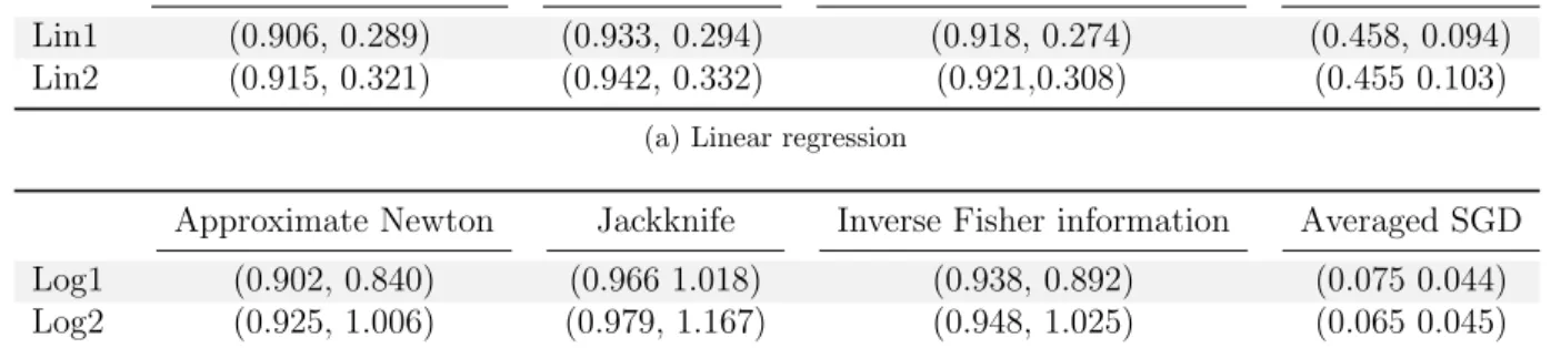
Approximate Newton Bootstrap Inverse Fisher information Averaged SGD Lin1 (0.906, 0.289) (0.933, 0.294) (0.918, 0.274) (0.458, 0.094) Lin2 (0.915, 0.321) (0.942, 0.332) (0.921,0.308) (0.455 0.103)

(a) Linear regression

Approximate Newton Jackknife Inverse Fisher information Averaged SGD Log1 (0.902, 0.840) (0.966 1.018) (0.938, 0.892) (0.075 0.044) Log2 (0.925, 1.006) (0.979, 1.167) (0.948, 1.025) (0.065 0.045)

(b) Logistic regression

Table 4.1: Synthetic data average coverage & confidence interval length for low dimensional problems.

Table 4.1 shows 95% confidence interval’s coverage and length of 200 simulations for linear and logistic regression. The exact configurations for linear/logistic regression examples are provided in Appendix2.1.1.1. Compared with Bootstrap and Jackknife [ET94], Algorithm1uses less numerical operations, while achieving similar results. Compared with the

(47)

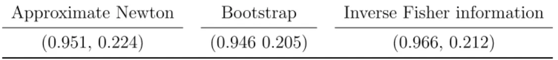
Approximate Newton Bootstrap Inverse Fisher information (0.951, 0.224) (0.946 0.205) (0.966, 0.212)

Table 4.2: Average 95% confidence interval (coverage, length) after calibration averaged SGD method [LLKC18, CLTZ16], our algorithm performs much better, while using the same amount of computation, and is much less sensitive to the choice hyper-parameters. And we observe that calibrated approximate Newton confidence intervals [ET94, PRW12] are better than bootstrap and inverse Fisher information (Table 4.2).

4.2.2 Real data

Neural network adversarial attack detection. Here we use ideas from statistical in-ference to detect certain adversarial attacks on neural networks. A key observation is that neural networks are effective at representing low dimensional manifolds such as natural images [BJ16, CM16], and this causes the risk function’s Hessian to be degenerate [SEG+₁₇_{]. From}

a statistical inference perspective, we interpret this as meaning that the confidence intervals in the null space of H+_GH+ _{is infinity, where} _H+ _{is the pseudo-inverse of the Hessian (see}

Chapter 4). When we make a prediction Ψ(x;θb) using a fixed data point x as input (i.e., conditioned on x), using the delta method [vdV98], the confidence interval of the prediction can be derived from the asymptotic normality of Ψ(x;θb)

√ nΨ(x;θb)−Ψ(x;θ?) →N0,_∇θΨ(x;θb)> h b H−1 b GHb−1 i ∇θΨ(x;θb) .

To detect adversarial attacks, we use the score

k(I−P_H+_GH+)∇θΨ(x;bθ)k

2

k∇θΨ(x;bθ)k

2

,

to measure how much_∇θΨ(x;θb) lies in null space ofH+GH+, whereP_H+_GH+ is the projection

(48)

image’s score should be larger than the original image’s score, and the adversarial image’s score should be larger than the randomly perturbed image’s score.

We train a binary classification neural network with 1 hidden layer and softplus activation function, to distinguish between “Shirt” and “T-shirt/top” in the Fashion MNIST data set [XRV17]. Figure 4.1 shows distributions of scores of original images, adversarial images generated using the fast gradient sign method [GSS14], and randomly perturbed images. Adversarial and random perturbations have the same`∞ norm. The adversarial perturbations

and example images are shown in Appendix 2.1.2.1. Although the scores’ values are small, they are still significantly larger than 64-bit floating point precision (2−53_≈₁_.₁₁_×₁₀−16_).

We observe that scores of randomly perturbed images is an order of magnitude larger than scores of original images, and scores of adversarial images is an order of magnitude larger than scores of randomly perturbed images.

0.2 0.4 0.6 0.8 1.0 1.2 score 1e 14 0.00 0.25 0.50 0.75 1.00 1.25 1.50 1.75 2.00 1e15 original 0 1 2 3 4 score 1e 12 0 1 2 3 4 5 1e12 adversarial random

Figure 4.1: Distribution of scores for original, randomly perturbed, and adversarially perturbed images

(49)

4.3 Statistical inference via approximate stochastic Newton steps

using first order information with increasing inner loop counts

Here, we present corollaries when the number of inner loops increases in the outer loops (i.e., (L)t is an increasing series). This guarantees convergence of the covariance estimate to

H−1_GH−1_{, although it is less efficient than using a constant number of inner loops.}

4.3.1 Unregularized M-estimation

Similar to Theorem 2’s proof, we have the following result when the number of inner loop increases in the outer loops.

Corollary 4. In Algorithm 1, if the number of inner loop in each outer loop (L)t increases in the outer loops, then we have

E " H−1_GH−1₋ So T T X t=1 ¯ gt¯g> t ρ2 t 2 # .T−do2 + v u u t1 T T X i=1 1 (L)t.

For example, when we choose choose (L)t = L(t + 1)dL _{for some} d

L > 0, then q 1 T PT i=1 1 (L)t =O( 1 √ LT −dL₂ ₎_.

4.4 SVRG based statistical inference algorithm in unregularized

M-estimation

Here we present a SVRG based statistical inference algorithm in unregularized M-estimation, which has asymptotic normality and improved bounds for the “covariance”. Although Algorithm 2has stronger guarantees than Algorithm 1, Algorithm 2requires a full gradient evaluation in each outer loop.

Corollary 5. In Algorithm 2, when L≥20max1≤i≤nβi

α and η=

1

(50)

Algorithm 2 SVRG based statistical inference algorithm in unregularized M-estimation 1: for t _←0;t < T; + +t do 2: d0 t ← −η∇f(θt) =−η n1 Pn i=1∇fi(θ)

// point estimation via SVRG 3: Io ← uniformly sampleSo indices with replacement from [n]

4: g0 t ← −ρt 1 So P i∈Io∇fi(θt) // statistical inference

5: for j ←0;j < L; + +j do // solving (4.1) approximately using SGD 6: Ii ← uniformly sampleSi indices without replacement from [n] 7: djt+1 ← d j t −η 1 Si P k∈Ii(∇fk(θt+d j t)− ∇fk(θt) +d0

t // point estimation via SVRG 8: gtj+1 ←g j t −τj 1 Si P k∈Ii 1 δjt [_∇fk(θt+δtjg j t)− ∇fk(θt)] +τjgt0 // statistical infer-ence 9: end for

10: Use √So· _ρg¯t_t for statistical inference // ¯gt= _L₊₁1 PL j=0g j t 11: θt+1 ←θt+ ¯dt // ¯dt= _L₊₁1 PL j=0d j t 12: end for

the outer loop, we have a non-asymptotic bound on the “covariance”

E " H−1_GH−1₋ So T T X t=1 ¯ gt¯g> t ρ2 t 2 # .L−12, (4.13)

and asymptotic normality

1 √ T( T X t=1 ¯ gt ρt ) = W + ∆, where W weakly converges to N(0, 1

SoH

−1_GH−1₎ _and _{∆ =}_o

P(1) when T → ∞ and L→ ∞

(_E[_k∆_k2]. √1_T +_L1).

When the number of inner loops increases in the outer loops (i.e., (L)t is an increasing series), we have a result similar to Corollary 4.

A better understanding of concentration, and Edgeworth expansion of the average consecutive iterates averaged (beyond [Dip08a, Dip08b]) in stochastic approximation, would