Building an Ensemble for Software Defect Prediction Based on Diversity Selection

(1)

Building an Ensemble for Software Defect Prediction

Based on Diversity Selection

Jean Petri´c

Science and Technology Research Institute University of Hertfordshire Hatfield, Hertfordshire AL10 9AB, UK

David Bowes

Tracy Hall

Department of Computer Science

Brunel University London Uxbridge, Middlesex

UB8 3PH, UK

Bruce Christianson

Nathan Baddoo

ABSTRACT

Background: Ensemble techniques have gained attention in various scientific fields. Defect prediction researchers have investigated many state-of-the-art ensemble models and con-cluded that in many cases these outperform standard single classifier techniques. Almost all previous work using en-semble techniques in defect prediction rely on the major-ity voting scheme for combining prediction outputs, and on the implicit diversity among single classifiers. Aim: Investi-gate whether defect prediction can be improved using an ex-plicit diversity technique with stacking ensemble, given the fact that different classifiers identify different sets of defects.

Method: We used classifiers from four different families and the weighted accuracy diversity (WAD) technique to exploit diversity amongst classifiers. To combine individual predic-tions, we used the stacking ensemble technique. We used state-of-the-art knowledge in software defect prediction to build our ensemble models, and tested their prediction abil-ities against 8 publicly available data sets. Conclusion: The results show performance improvement using stacking ensembles compared to other defect prediction models. Di-versity amongst classifiers used for building ensembles is es-sential to achieving these performance improvements.

Keywords

Software defect prediction, software faults, ensembles of learn-ing machines, stacklearn-ing, diversity

Permission to make digital or hard copies of all or part of this work for personal or classroom use is granted without fee provided that copies are not made or distributed for profit or commercial advantage and that copies bear this notice and the full cita-tion on the first page. Copyrights for components of this work owned by others than ACM must be honored. Abstracting with credit is permitted. To copy otherwise, or re-publish, to post on servers or to redistribute to lists, requires prior specific permission and/or a fee. Request permissions from [email protected].

1. INTRODUCTION

A software defect can cause programs to misbehave, lead-ing to negative effects for the software industry. Defects that are fixed pre-release can potentially save companies from high repair costs and a bad reputation. The software in-dustry spends billions of pounds annually finding and fixing defects. Defect prediction assists practitioners to promptly identify parts of software likely to contain defects, and act accordingly before the system is delivered to users. Predic-tion modelling has been used in several hundred studies con-ducted in software defect prediction in the last few decades. Some of the most recent work in software defect prediction literature has been covered in several meta-analysis and sys-tematic literature reviews [2, 7, 12, 30].

As a matter of usual practice, researchers have used dozens of publicly available defect data sets, and tested different modelling techniques on those data sets. The standard ap-proach to defect prediction is to use historical data con-taining quantitative measures about software modules. The historical data is fed into machine learners that produce pre-diction models. These prepre-diction models can then be used to determine which software instances contain defects, by pro-viding them new instances for which the defectiveness status is unknown to a model. Menzies et al. hypothesized that the current standard approaches used in defect prediction have reached their limits, and that new approaches are needed to make better predictions [14]. In this work, we focus on using ensemble techniques to make improved predictions.

Existing defect prediction studies generally do not con-sider whether different models find different sets of defects. Lessmann et al. did a study using 22 different machine learn-ers, and concluded that the top 18 classifiers perform simi-larly [11]. The result that the majority of classifiers perform similarly suggests that it does not matter which classifiers are chosen to build prediction models. Similar average re-sults that various classifiers produce could potentially hide different sets of defects that they identify. However, not all defects are the same. Diverse mathematical properties underlying different classifiers may have an effect on which

(2)

defects are found by one classifier, and not by others. Re-cently, Panichella et al. have confirmed that in cross-project defect prediction different techniques could be combined to find a wider range of defects than by just using single classi-fiers [17]. In within-project defect prediction, we previously confirmed that different machine learners detect very differ-ent subsets of defects [1]. Therefore, we now aim to iddiffer-entify whether different machine learners, when combined, can en-hance the performance of prediction models.

To achieve our aim, we performed an experiment to es-tablish whether ensemble techniques based on diversity and stacking can improve defect prediction. Ensembles of ma-chine learners combine multiple classifiers and join their pre-diction outputs into a final solution. It is widely accepted by the machine learning community that ensemble mod-els should contain diverse classifiers and that their outputs should be combined in a way that will amplify the correct decisions of single classifiers. Some ensemble techniques (e.g. Bagging) implicitly achieve diversity amongst classifiers by randomising a data set in each iteration of the algorithm. Since base classifiers are trained on different training sets, each classifier should make different predictions. In this case, the diversity amongst different classifier families is not ac-counted for. However, it is likely that ensemble modelling can be improved in the context of defect prediction. We use an explicit diversity scheme, which targets only the most di-verse predictors from several different families to build our ensembles, since different classifiers discover different sub-sets of defects [1, 17]. Schemes like majority voting may not be suitable for defect prediction as unique subsets of defects are identified by some classifiers and not by others, making majority voting a non-optimal approach for combining en-semble outputs. Therefore, we use the stacking technique. Stacking performs a classification task with the prediction results previously made by individual classifiers. The output produced by this classification task gives the final prediction. Particularly, we want to address the following research ques-tions:

RQ1 Can stacking ensembles based on explicit diversity im-prove prediction performance compared to other defect prediction models?

RQ2 How many classifiers combined into stacking

ensem-bles provide good defect prediction models?

RQ3 How much diversity and which base classifiers are usu-ally combined in stacking ensemble models?

In this work we make several contributions. First, we show that ensemble models based on classifiers from different fam-ilies can improve defect prediction. We further explore how much diversity affects defect prediction models and what are the most popular classifiers chosen for building the stacking ensembles. We also show that only a few, but diverse classi-fiers, are sufficient to build effective ensemble models. This knowledge could help other researchers and practitioners to build improved defect prediction models.

Our paper is structured as follows. In the next section, we give an overview of software defect prediction and ensemble techniques. In the third section we detail our methodology followed by the results and discussion in the fourth section. We present the threats to validity of our experiment in the fifth section, give conclusiouns in the sixth section, and in-troduce ideas for future work in the seventh section.

2. BACKGROUND

Software defect prediction uses independent and depen-dent variables, and mathematical models to predict error-prone locations in software. Independent variables are quan-titative measures of software, generally depicting the size and complexity of its components. Size, complexity, and CK object-oriented are the most common metrics used in studies of defect prediction [12]. Fenton and Neil showed that size is in a complex relationship with defects, resulting in studies that range from size giving good prediction to very poor prediction results [3]. Shepperd criticised complexity measures as being a proxy for several other metrics used in defect prediction [23]. Much effort has been put to engi-neering new metrics for defect prediction. Recently, Shippey presented a new metric based on the Java abstract syntax tree and showed usefulness in predicting a specific subsets of defects [26]. Zimmermann and Nagappan used graph theory, showing that software modules with a greater degree of cen-trality tend to be more defective [37]. Similarly, Petri´c and Galinac used graph theory to show that some graph struc-tures are more related to defects than others [19]. However, there is no definite agreement about which metric is superior for defect prediction. Most defect prediction studies tend to use a combination of available metrics.

Independent variables are usually combined with depen-dent variables in the form of a data set. Each data set contains a set of software units (modules), where each mod-ule is described with its metrics (independent variables) and the corresponding defectiveness (dependent variable). The dependent variable can be a number depicting the density of defects contained in a module, or a flag stating whether a module is defective or not. The systematic collection

of such data is a complex and time consuming task. To

tackle this problem, the PROMISE repository has been es-tablished containing a collection of publicly available defect

data. Although very popular, some PROMISE data sets

have been shown to be of low quality [5, 18]. However,

for the sake of comparability with other studies, many re-searchers have used the original versions of the data sets available at PROMISE [7].

Researchers mostly use machine learning classifiers in the context of defect prediction [30]. Classifiers are first trained by using historical defect data, and then exploited to make predictions on the new data, previously not seen by a model [28, 33]. Lessmann et al.’s comprehensive study, which was performed using 22 different classifiers, showed no signifi-cant difference among the top 18 classifiers [11]. Lessmann et al. have presented average figures for the prediction per-formances of their classifiers. We showed that these perfor-mance figures hide the sets of defects identified by using dif-ferent prediction models [1]. Specifically, we demonstrated that different classifiers are capable of finding different de-fects, where some subsets of defects are unique to a specific classifier. Panichella et al.’s study reported similar conclu-sions in the context of cross-project defect prediction [17].

Following our findings, and those of Panichella et al., we explore the use of ensembles of machine learners. The idea of ensemble models is to combine multiple single classifiers with the aim of improving the predictive performance of single classifiers [15, 21]. In the last few years, ensembles of machine learners have been occasionally used in software defect prediction. One of the fundamental motivations for using ensembles is the performance bottleneck [14] when

(3)

us-ing sus-ingle classifiers. Wang et al. conducted a comparison study between popular ensemble classifiers and some single classifiers [31]. They showed that in many cases ensemble classifiers outperform other classifiers, including the single Na¨ıve Bayes algorithm. Kultur et al. presented an ensemble of neural networks with associative memory that achieve more accurate and stable results compared to neural net-works themselves [8]. More recent work also demonstrates the efficacy of ensemble learners against more conventional methods such as Support Vector Machines [10]. Particularly, Laradji et al. demonstrated that ensemble classifiers made up of carefully devised learners and using a few useful fea-tures can achieve improved results over other conventional models. The reasons for using ensembles in predictive mod-elling are covered in detail by Polikar [20].

Two things should be carefully considered when building ensemble models. First, ensembles should be built from di-verse classifiers. Ensembles should include classifiers that make different incorrect predictions (because classifiers that make the same prediction errors do not add any informa-tion). Second, combining the outputs from all classifiers should be done in a way that encourages the correct decisions are amplified and ignores incorrect decisions. Since different classifiers find different defects, techniques commonly used in defect prediction for combining classifier outputs, such as majority voting, should be reconsidered. Current ensem-ble models in software defect prediction are not specifically designed to combine prediction outputs in such a way that will amplify correct predictions. If several prediction models have uniquely identified different sets of defects, then ma-jority voting will not be a suitable technique to increase pre-diction performance. On the contrary, some of the defects uniquely identified by single classifiers will now be misclas-sified, downgrading the overall performance of the ensemble models. Combining the decisions of individual classifiers can be achieved using other techniques rather than majority vot-ing. In this study, we use the stacking approach first intro-duced by Wolpert [34]. Stacking uses a two layer approach, where the first layer is constituted of individual classifiers, all trained on the same training data. The second layer, also called the meta layer, uses the output predictions of individ-ual classifiers from the first layer as an input. This input is fed into the second layer classifier which then makes the final predictions. Therefore, the stacking approach seeks patterns in predictions made by the first layer, rather then ignoring classifiers that have minority “votes”. Consequently, if a specific subset of defects is detectable only by one classifier, stacking will still have an opportunity to correctly classify such instances. The majority-voting approach would cer-tainty misclassify such instances, since all but one of the classifiers would predict non-defective.

Many techniques for measuring and achieving higher di-versity have been proposed by Kuncheva and Whitaker [9]. Some of these measures are Correlation diversity,Q-statistics, Disagreement and Double Fault Measures, Entropy Mea-sures, Kohavi-Wolpert Variance, Weighted Accuracy and Diversity (WAD), etc. Kuncheva and Whitaker argue that there is no diversity measure that consistently correlates with higher accuracy. They recommend the use ofQ-statistics because of its simplicity and intuitive meaning. WAD is an-other relatively simple diversity measure proposed by Zeng et al. [35], who showed that using WAD in combination with a bagging approach can boost prediction performance.

We use WAD in this work as a diversity measure in defect prediction.

3. METHODOLOGY

3.1 Data sets

We used several public data sets from PROMISE1_{, the}

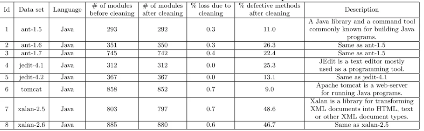
repository commonly used by researchers in software defect prediction. We selected 8 data sets shown in Table 1, which come from different domains, to ensure diversity among pos-sible defects that can appear in each project. We performed data cleaning to remove software modules that comply with the following rules:

• LOC= 0

• AnyN umericalM etric <0

• CCavg> CCmax

• N OC > LOC • N P M > W M C

We remove instances where lines of code (LOC) is 0, or any numerical metric is negative as suggested by Shepperd et al. [25]. We additionally remove instances where the average cyclomatic complexity (CCavg) exceeds the maximal cyclo-matic complexity (CCmax), number of comments (NOC) is greater than number of lines of code and number of public methods for a class (NPM) is greater than weighted methods per class (WMC).

3.2 Base classifiers

We experimented with four different classifiers, namely Na¨ıve Bayes , C4.5 decision tree, K-nearest neighbour, and sequential minimal optimisation. These four were chosen since classifiers from different “families” were previously suc-cessful in finding different defects [1, 17]. Na¨ıve Bayes be-longs to a family of linear classification techniques, where the prediction of a model is made according to conditional probabilities. It requires all variables to be categorical and assumes full independence among them. C4.5 is a tree-based learning algorithm that produces a structured classification model on which all predictions are based. The C4.5 algo-rithm uses information theory to make an optimal decision about node splitting on the attribute which best separates the data. K-nearest neighbour makes predictions based on the class values of closest neighbours. It uses a distance algorithm to findK nearest neighbours of the instance be-ing predicted, and then assigns to that instance the highest occurring class of its neighbours. Sequential minimal opti-misation is used for training Support Vector Machines in a more nearly optimal way than its predecessor algorithms. Support Vector Machine algorithms are designed for solving non-linear problems by mapping data points into a higher-dimensional space and separating the classes with a linear hyper-plane. The hyper-plane is usually chosen to maximise the distance between classes.

From each base classifier we have built several different models, changing the classifier parameters to address two important ideas. First, parameter tuning has been shown

1

(4)

Table 1: PROMISE data sets used in our experiment

Id Data set Language # of modules before cleaning # of modules after cleaning % loss due to cleaning % defective methods

after cleaning Description 1 ant-1.5 Java 293 292 0.3 11.0

A Java library and a command tool commonly known for building Java

programs. 2 ant-1.6 Java 351 350 0.3 26.3 Same as ant-1.5 3 ant-1.7 Java 745 742 0.4 22.4 Same as ant-1.5 4 jedit-4.1 Java 312 312 0.0 25.3 JEdit is a text editor mostly

used as a programming tool. 5 jedit-4.2 Java 367 367 0.0 13.1 Same as jedit-4.1 6 tomcat Java 858 852 0.7 9.0 Apache tomcat is a web-server

for running Java programs. 7 xalan-2.5 Java 803 797 0.7 48.6

Xalan is a library for transforming XML documents into HTML, text or other XML document types. 8 xalan-2.6 Java 885 880 0.6 46.7 Same as xalan-2.5

to have an important role when building prediction mod-els [6, 27]. Support Vector Machine classifiers are known to perform badly if not tuned. Decision trees might produce over-optimistic models if the number of possible branches is unlimited. K-nearest neighbour has problems with unbal-anced data since the probability of predicting the majority class is higher. Na¨ıve Bayes can use different kernel estima-tors to convert continuous into nominal data. Second, dif-ferent parameters enrich diversity among classifiers, possibly making mistakes in different instances, which is a valuable

characteristic when building ensembles [20]. When more

classifiers make mistakes on different instances, a strategic combination of these classifiers may reduce the total error. In total, 15 base classifiers were used, each coming from one of the four families and using different model parameters.

We used two different parameters for a Na¨ıve Bayes (NB)

learner. One parameter uses a kernel density estimator

rather than normal distribution for continuous attributes. The second parameter uses supervised discretisation for pro-cessing continuous attributes. The purpose of both parame-ters is to best split continuous attributes into nominal ones, since the Na¨ıve Bayes classifier works only with categorical values. Two different parameters are usually tuned inK -nearest neighbour (kNN) learners, thek value and the near-est neighbour searching algorithm. The first parameter,k, denotes how many nearest neighbours the algorithm should take into consideration. Thek parameter should be an odd number higher than 0. We chose three different values: 3, 5 and 7. Further increase of the parameterk may have a negative impact on our learners since defect prediction data is generally imbalanced. We left the default value for the nearest neighbour searching algorithm, which is the Euclid-ian distance. For the Support Vector Machines algorithm we have used sequential minimal optimisation (SMO). SMO uses less complex methods than its predecessors for train-ing support vector machines, providtrain-ing for the creation of faster models. For SMO we varied the complexity param-eter C, assigning four different values: 1, 10, 25 and 50. The complexity parameterC controls the margin that sep-arates the defective instances from the non-defective ones. If theC parameter is very small, the SMO algorithm will try to maximise the margin between two classes. On the other hand, higherC values will force the SMO algorithm to find margins that make the least amount of mistakes on the training data. Consequently, increasing the C values

can lead to over-fitting, since the margin is tightly adjusted to the training data. Other parameters for SMO were left at their default values. The last family of classifiers is decision tree. The Weka implementation of decision tree is called J48. We varied the confidence factor of the J48 classifier using five different values: 0.25, 0.20, 0.15, 0.10, 0.05. Low-ering the confidence factor, the J48 classifier will result in more pruning.

3.3 Diversity

Diversity is one of the key components when building en-semble models. Having multiple classifiers that make mis-takes on the same instances does not add any additional in-formation that we did not have with only a single classifier. Therefore, when building ensemble models, diversity should ensure that we include only classifiers that make mistakes on different instances. The common and simplest way of calculating diversity measures is between each pair of clas-sifiers. An overall diversity is then calculated by averaging these pair-wise values. Several measures are frequently used to measure the diversity between pairs of classifiers. Corre-lation diversity measures the diversity between each pair of classifiers by obtaining the correlation between two classi-fier outputs. TheQ-Statistic gives positive values when two classifiers make correct predictions, negative values for in-correct predictions and 0 for the maximal diversity between classifiers. Weighted accuracy and diversity (WAD), intro-duced by Zeng et al. [35], belongs to the family of diversity measures that compare two classifiers at a time. The WAD measure works on a similar principle to the F-measure by finding a weighted harmonic mean between accuracy and diversity:

W ADα,β(Acc, Div) =

Acc·Div

β·Acc+α·Div (1)

whenα+β= 1.Theαandβparameters represent weights that control the importance of accuracy and diversity, where

α > βgives more focus on accuracy, andα < βfocuses more on diversity. Whenα > β, the WAD measure combines mul-tiple classifiers that are more accurate rather than diverse, and vice versa. In our experiment the accuracy in the WAD equation was replaced with precision, since accuracy is not a suitable measure for imbalanced data sets commonly found in SDP [4].

(5)

Diversity was computed among all pairs of classifiers as: Div= 2 m(m−1) m−1 X i=1 m X j=i+1 divi,j (2)

where m denotes the number of base classifiers in an en-semble, and i, j indexes of each base classifier. Diversity between each pair of classifiersdivi,j was calculated using the following equation:

divi,j=

N10₊_N01

N00₊_N11₊_N10₊_N01 (3)

where N11 represents the correct prediction of both clas-sifiers, andN10 _{the situation where classifier}_i _{makes the}

correct prediction whilst classifierjincorrect. N00 denotes incorrect prediction of both classifiers, and finallyN01 de-picts correct prediction of the classifierj, but incorrect pre-diction of the classifieri.

3.4 Experimental setup

We used Song et al.’s and Gray’s software defect predic-tion frameworks to build our predictors [6, 28]. The frame-work is divided into two parts, a scheme evaluation stage and a defect prediction stage. The scheme evaluation stage eval-uates the performance of different classifiers to find the best prediction models among all classifiers. At this stage only training data is used, which is further split into the training' and validation sets. The test set is left out from the eval-uation stage and used in the next, defect prediction stage. The defect prediction stage consists of the final prediction model that uses the test set for evaluating the model perfor-mance. Each experiment is run using 10 times 10 fold strat-ified cross-validation. Repeating an experiment 10 times, as well as using cross-validation, reduces the amount of vari-ance in the evaluation of prediction models. The stratified technique guarantees the same distribution of the minority and the majority class as in the original data for each fold, preventing folds constituted only from the majority class. To ensure that we use only relevant attributes, we performed correlation-based feature selection on all training sets. A subset of attributes for each fold was recorded, and applied on the test set at the defect prediction stage.

Base learners can be combined in many different ways, as well as made up of a lot of different classifiers, however for an optimal model this step should be carried out with care. Although ensembles have still not been extensively used in software defect prediction, until now researchers have usu-ally used some sort of majority voting as a decision making rule for ensembles [16, 22]. However, we showed in our previ-ous work that using majority-like voting mechanisms results in some defects being ignored by such ensembles [1]. Simi-larly to Panichella et al. [17], we proposed the stacking ap-proach when building ensemble based prediction models for software defect prediction. Still, combing all base learners into stacking may not be computationally and performance-wise optimal. More classifiers in an ensemble will inevitably prolong experiments, but it will not simultaneously guar-antee better performance results. To address this issue, we selected only a subset of classifiers in a way that is explanied below.

Our stacking ensembles were built using 5 different mea-sures depicted in Table 2. Each stacking ensemble was pro-duced by combining multiple base classifiers according to

Table 2: Measures used for building ensemble mod-els

Measure Full name Type of measure

1 BASE No measure Basic

2 PRECISION Precision Base

3 MCC Matthews correlation coeficient Base

4 DIV Diversity Advanced

5 WAD WAD Advanced

their measure stated in Table 2. Precision and MCC

be-long to the basic group of measures, directly provided by the Weka API. For instance, when stacking is built using precision, only the most precise classifiers are put into the

ensemble. Similarly for the other Basic measures. WAD

and Div measures are part of the Advanced group of mea-sures. These measures are not provided by the Weka API, rather are derived from Equations 1 and 2, respectively. The last measure isBase. Baseindicates one base classifier that performs best among all the other base classifiers.

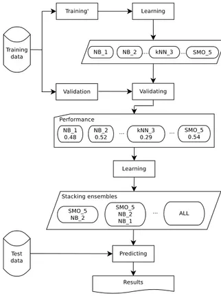
Figure 1: Stacking building

Figure 1 depicts the design used for building our stack-ing models. All base classifiers were first trained on the training’ data sets, and evaluated using the validation set. Performances on the validation set were further sorted from the highest to the lowest value for each performance mea-sure stated in Table 2. Starting from Precision, each mea-sure was then taken to form a stacking ensemble. The two most precise base classifiers were taken to form the stack-ing ensemble. The model was trained on the whole trainstack-ing set, and finally evaluated on the test set. The experiment continued combining the three most precise base classifiers, forming the stacking ensemble, training on the whole train-ing set and evaluattrain-ing on the test set. After combintrain-ing all

(6)

base classifiers, the experiment carried on the next measure from Table 2,MCC. The specialBasegroup was evaluated slightly differently. Each base classifier was directly trained on the whole training set, and evaluated on the test set.

3.5 Performance measure

There has been a great debate on measuring the perfor-mance of prediction models [4, 13, 36]. When quantifying the performance of classifiers based on a categorical depen-dent variable, usually some performance measure, derived from confusion matrix, is reported. The confusion matrix is depicted in Table 3. However, some performance measures

Table 3: Confusion matrix

Predicted defective Predicted defect free Observed defective True Positive (TP) False Negative (FN) Observed defect free False Positive (FP) True Negative (TN)

are not suitable for use in the defect prediction context. De-fect prediction data is commonly imbalanced, which makes some performance measures unusable (e.g. probability of detection [36]). On the other hand, frequently used mea-sures such as precision and recall do not take all four quad-rants into consideration, leaving space for making incorrect conclusions. Matthews correlation coefficient (MCC) is an appropriate measure when it comes to imbalanced data sets, and it captures all four quadrants of the confusion matrix [24]. MCC ranges from -1 to 1, where -1 indicates perfect disagreement, whilst 1 indicates perfect agreement between prediction and observation. The MCC value of 0 represents prediction no better than random. Given that MCC cap-tures all quadrants of the confusion matrix, we believe that this measure is a trustworthy indicator of the prediction per-formance.

4. RESULTS AND DISCUSSION

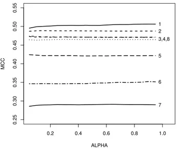
We conducted a series of experiments to build the final ensemble models. Since we used the WAD measure, proper tuning ofα andβ parameters depicted in Equation 1 was required. Therefore, we ran a set of prediction models on all data sets changing both parameters. The parameters were changed in the range from 0 to 1 in steps of 0.05. They -axis on Figure 2 depicts the change in MCC performance for all data sets we used. Thex-axis represents the value ofα

parameter, whereβ parameter was changed automatically to satisfyα+β= 1.

Figure 2 shows no compelling difference in MCC amongst all the data sets we used by changing the WAD param-eters. The greatest differences were achieved on margins whereα= 0 andα= 1. However, marginal values have al-ready been covered usingPrecisionandDiversity measures. Use of Precision can be compared to α = 1 since in this case diversity is ignored. Similarly, when α= 0 Precision is completely ignored and focus is on the diversity among base classifiers. Considering bothPrecision and Diversity as important factors when building ensembles, we set both parameters to 0.5. Settingα=β= 0.5 ensures that both concepts are equally represented.

Table 4 shows the average performance values of single and ensemble classifiers. The columns contain different pre-diction techniques, whilst rows depict average MCC and

0.2 0.4 0.6 0.8 1.0 0.25 0.30 0.35 0.40 0.45 0.50 0.55 ALPHA MCC 7 6 5 3,4,8 2 1

Figure 2: WAD sensitivity for all eight data sets

Table 4: Average MCC performance across all data sets

Data set SC BA BO PR MCC DIV WAD

ant-1.5 Avg. 0.255 0.338 0.303 0.461 0.485 0.507 0.503 Dev. 0.276 0.285 0.287 0.254 0.246 0.24 0.242 ant-1.6 Avg. 0.408 0.479 0.412 0.475 0.49 0.488 0.488 Dev. 0.174 0.145 0.168 0.154 0.148 0.145 0.145 ant-1.7 Avg. 0.395 0.456 0.389 0.448 0.474 0.465 0.465 Dev. 0.134 0.124 0.128 0.131 0.131 0.123 0.123 jedit-4.1 Avg. 0.427 0.433 0.403 0.459 0.466 0.471 0.471 Dev. 0.191 0.187 0.181 0.185 0.178 0.182 0.182 jedit-4.2 Avg. 0.334 0.338 0.342 0.346 0.426 0.421 0.421 Dev. 0.243 0.219 0.217 0.232 0.191 0.193 0.193 tomcat Avg. 0.171 0.247 0.23 0.3 0.349 0.351 0.348 Dev. 0.192 0.203 0.175 0.177 0.156 0.153 0.158 xalan-2.5 Avg. 0.257 0.355 0.35 0.274 0.293 0.29 0.29 Dev. 0.115 0.108 0.1 0.109 0.107 0.107 0.106 xalan-2.6 Avg. 0.474 0.535 0.495 0.471 0.471 0.471 0.471 Dev. 0.089 0.08 0.093 0.092 0.092 0.092 0.092 Avg. 0.34 0.398 0.366 0.404 0.432 0.433 0.432 Dev. 0.177 0.169 0.169 0.167 0.156 0.154 0.155

standard deviation values for each data set. To make our approach more readily comparable to other approaches, we trained two additional ensemble models commonly used in SDP, namely Bagging and Boosting. Both additional models were trained using the same parameters for the base classi-fiers as described in Section 3.2. SC represents the average values of all 15 single classifiers used, whilst BA and BO are the bagging and boosting approaches added for compar-ison, respectively. The rest of the table represents the other basic and advanced measures used,Precision,MCC, Diver-sity, andWAD, respectively. Average performance measures show that across all data sets our techniques achieve better results than the other approaches. Particularly, the aver-age figures from Table 4 show that the DIV technique is better by 27.2%,Bagging by 8.9%, andBoosting by 18.5% compared to theSingle classifiertechnique. For formal con-firmation in favour of theDIV technique, we used Wilcoxon signed-rank test to statistically compare the differences [32]. The same form of test was previously used by Sun et al. in the context of defect prediction [29]. The alternative hy-pothesis tests whether for a given technique (single clas-sifier OR baggingOR boosting), DIV technique performs

(7)

better than the other three techniques at significance level

α= 0.05. Thep-values of theSingle Classifier and Boost-ing techniques were less than 0.05, whilst the p-value for the Bagging technique was greater than 0.05. From these results we can conclude that theDIV technique is signifi-cantly better than the other techniques exceptBagging. The same conclusions were derived for the WAD and MCC tech-niques using the same statistical approach.

Table 5: Relative increase in true positives of all techniques compared to Bagging

BA SC BO PR MCC DIV WAD ant-1.5 1.06 -0.20 -0.07 0.68 0.83 0.94 0.93 ant-1.6 4.95 -0.10 -0.02 0.09 0.20 0.22 0.21 ant-1.7 8.02 -0.11 -0.02 -0.00 0.21 0.24 0.24 jedit-4.1 3.65 -0.03 0.08 0.08 0.18 0.24 0.24 jedit-4.2 1.53 -0.03 0.14 0.24 0.78 0.78 0.78 tomcat 1.40 -0.08 0.31 1.28 2.01 2.02 2.03 xalan-2.5 25.21 -0.15 0.02 -0.20 -0.05 -0.08 -0.08 xalan-2.6 28.99 -0.11 0.02 -0.25 -0.19 -0.18 -0.18 Avg 9.35 -0.10 0.06 0.24 0.50 0.52 0.52

Table 6: Relative increase in false positives of all techniques compared to Bagging

BA SC BO PR MCC DIV WAD ant-1.5 1.01 0.19 0.14 0.87 1.07 1.15 1.17 ant-1.6 2.50 0.16 0.38 0.31 0.55 0.62 0.62 ant-1.7 4.41 0.16 0.41 0.09 0.54 0.73 0.72 jedit-4.1 1.95 -0.03 0.44 0.06 0.32 0.46 0.46 jedit-4.2 1.46 -0.06 0.41 0.49 1.35 1.45 1.45 tomcat 1.50 0.54 1.26 3.35 4.82 4.86 4.95 xalan-2.5 12.26 0.00 0.05 -0.13 0.09 0.05 0.05 xalan-2.6 8.35 -0.04 0.27 -0.45 -0.28 -0.25 -0.25 Avg 4.18 0.11 0.42 0.57 1.06 1.14 1.15

Having established the average performances of our mod-els, we further investigated the effect size of all approaches. The effect size serves as a measure of how many defects can each model detect (true positives) for the price of misclas-sifying certain instances (false positives). To demonstrate effect sizes, we derived the confusion matrix for all runs and across all data sets. To make our comparison fair, we com-paredSingle Classifier,Boosting,Precision,MCC,DIV, and WAD against theBaggingtechnique. The reason for this is that theBaggingtechnique achieved better results than Sin-gle Classifier andBoosting. Also, we want to compare our techniques against others that achieve best results in defect prediction. The first column in Table 5 shows the average number of true positives achieved byBagging. The follow-ing columns show the relative increase in the number of true positives for the techniques used in our study. Clearly,DIV andWADtechniques achieve better performances relative to Single Classifiers,Bagging and Boosting techniques. More precisely,DIV andWAD techniques can on average achieve a relative increase of 0.52 compared to the Bagging tech-nique. For instance, in the case of the tomcat data set, the WAD technique correctly identifies about two times more defects relative toBagging. Table 6 on the other hand de-picts an increase of false positives. Taken together, the ta-bles of relative increase in true and false positives show that there is a trade-off between true positives and false posi-tives. However, increasing the number of true positives in defect prediction is particularly challenging since data sets are known to be imbalanced. Although a higher false posi-tive rate detection is discouraged, finding more real defects

for the price of more false positives could be of benefit for some companies. This is especially true for companies where the cost of defects is extremely high.

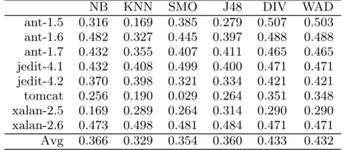
We additionally compared single classifiers against our best two techniques, DIV and WAD. The reason is a fre-quent use of single classifiers in SDP. To make a fair com-parison, we extracted only one classifier from each family that on average achieved the best MCC performance. From

Table 7: Average best single classifiers against DIV and WAD

NB KNN SMO J48 DIV WAD

ant-1.5 0.316 0.169 0.385 0.279 0.507 0.503 ant-1.6 0.482 0.327 0.445 0.397 0.488 0.488 ant-1.7 0.432 0.355 0.407 0.411 0.465 0.465 jedit-4.1 0.432 0.408 0.499 0.400 0.471 0.471 jedit-4.2 0.370 0.398 0.321 0.334 0.421 0.421 tomcat 0.256 0.190 0.029 0.264 0.351 0.348 xalan-2.5 0.169 0.289 0.264 0.314 0.290 0.290 xalan-2.6 0.473 0.498 0.481 0.484 0.471 0.471 Avg 0.366 0.329 0.354 0.360 0.433 0.432

the Na¨ıve Bayes family, the classifier with a kernel density estimator achieved the best MCC result in average across all data sets. K nearest neighbour with k= 3, SMO with

C = 50, and J48 with C = 0.10 achieved the best aver-age performances according to MCC. Single classifiers with

the best average MCC performances, along with DIV and

WADtechniques are shown in Table 7. SinceDIV andWAD both achieved the same average MCC performances, they improved over Na¨ıve Bayes by 18.2%, overKNN by 31.4%, over SMO by 22.3%, and finally over J48 by 20.1%. The Wilcoxon significance test, where the alternative hypothesis

tests superior performance values of DIV and WAD over

Single Classifierswas performed. With thep= 0.05 level of confidence we confirmed that the both techniques,DIV and WAD, are superior to all the other Single Classifier tech-niques.

RQ1. Can stacking ensembles based on ex-plicit diversity improve prediction perfor-mance compared to other defect prediction models?

From the analysis of MCC performance and rela-tive improvements in effect sizes we can conclude that stacking ensembles can indeed improve predic-tion performance.

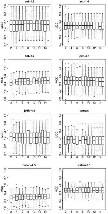
In our final experiment we test how many classifiers, and of which family, used for building stacking ensembles are needed for these ensembles to perform well. It may be the case that combining only a few classifiers, that are most precise and diverse, is sufficient for achieving good perfor-mance results. This would have practical benefits reducing the training time of such ensemble classifiers. Since we built stacking ensembles of all possible sizes (combining from 2 to 15 single classifiers used in this study), it is now possible to compare their prediction performances. Furthermore, it is possible to analyse which single classifiers are often picked by the ensemble. In the context of this analysis, we inves-tigate only the WAD technique, since it is based on both aspects that are in the focus of our analysis: diversity and precision. Additionally, the WAD technique performed as

(8)

MCC 2 4 6 8 10 12 14 0.0 0.2 0.4 0.6 0.8 1.0 ant−1.5 MCC 2 4 6 8 10 12 14 0.0 0.2 0.4 0.6 0.8 1.0 ant−1.6 MCC 2 4 6 8 10 12 14 0.0 0.2 0.4 0.6 0.8 1.0 ant−1.7 MCC 2 4 6 8 10 12 14 0.0 0.2 0.4 0.6 0.8 1.0 jedit−4.1 MCC 2 4 6 8 10 12 14 0.0 0.2 0.4 0.6 0.8 1.0 jedit−4.2 MCC 2 4 6 8 10 12 14 0.0 0.2 0.4 0.6 0.8 1.0 tomcat MCC 2 4 6 8 10 12 14 0.0 0.2 0.4 0.6 0.8 1.0 xalan−2.5 MCC 2 4 6 8 10 12 14 0.0 0.2 0.4 0.6 0.8 1.0 xalan−2.6

Figure 3: Prediction performance of WAD groups of classifiers. Thex-axis represents the size of a group.

well as our other ensemble techniques. Figure 3 presents prediction performance box-plots for all 8 data sets used in our analysis. Thex-axis depicts the size of each group us-ing the WAD technique, whilst they-axis shows the MCC performance. From the figure it is clear that small groups, of just two or three classifiers, combined into the stacking ensemble perform well. Combining only three classifiers into a stacking ensemble gives prediction performance not signif-icantly worse than combining more classifiers, as Figure 3 demonstrates. This statement is valid for all data sets used in our experiment. Achieving such results is important since training only three classifiers, and using an additional classi-fier in the stacking meta-layer, reduces the time for building

a prediction model.

RQ2. How many classifiers combined into stacking ensembles provide good defect pre-diction models?

Our experiment showed that adding more than three classifiers into the stacking ensembles does not sig-nificantly increase the prediction performance.

Table 8: Frequency of the individual classifiers ap-pearing in the stacking ensembles of size 3

# Data set Classifier Frequency (%)

1 ant-1.5 NB default parameters 100

2 ant-1.5 SMO -C 1, else default parameters 90 3 ant-1.5 kNN k=3, else default parameters 34 1 ant-1.6 SMO -C 1, else default parameters 100 2 ant-1.6 kNN k=3, else default parameters 85

3 ant-1.6 NB -D 77

1 ant-1.7 NB -D 100

2 ant-1.7 SMO -C 1, else default parameters 100 3 ant-1.7 kNN k=3, else default parameters 99

1 jedit-4.1 NB -D 100

2 jedit-4.1 SMO -C 1, else default parameters 95 3 jedit-4.1 kNN k=3, else default parameters 90

1 jedit-4.2 NB -D 100

2 jedit-4.2 SMO -C 1, else default parameters 89

3 jedit-4.2 NB default parameters 59

1 tomcat NB -D 100

2 tomcat kNN k=3, else default parameters 45

3 tomcat NB default parameters 44

1 xalan-2.5 kNN k=3, else default parameters 83 2 xalan-2.5 SMO -C 1, else default parameters 56 3 xalan-2.5 J48 -C 0.25, else default parameters 41 1 xalan-2.6 kNN k=3, else default parameters 97

2 xalan-2.6 NB -D 95

3 xalan-2.6 NB default parameters 86

Finally, we investigated the base classifiers that form our stacking ensemble in order to find the ones that are fre-quently chosen by ensembles. For the purpose of this analy-sis we again used the WAD technique with stacking ensem-bles of size 3. Table 8 shows the first three classifiers com-monly used for building stacking ensembles for all 8 data sets used. The Na¨ıve Bayes classifier has constantly been chosen by the stacking ensemble, with an average frequency of 86% across all data sets. This suggests that Na¨ıve Bayes classifiers perform well across all data sets, and increase di-versity in ensembles. Some variants of SMO have also been repeatedly chosen by stacking ensembles, often with differ-ent parameter settings. Interestingly, the frequdiffer-ently used decision tree classifier J48 was not dominant for any of the data sets.

RQ3. How much diversity and which base classifiers are usually combined in stacking ensemble models?

Although only a small proportion of classifiers are needed to build a stacking ensemble that performs well, diversity among classifiers seems to have an important role in this. The frequency table (shown in Table 8) suggests that the ensembles of size 3 are usually combined with classifiers from different families (e.g. in 90% of the runs Na¨ıve Bayes , SMO and kNN combine together in ensembles for Jedit-4.1).

(9)

5. THREATS TO VALIDITY

We consider several internal and external threats to valid-ity. In our study, we replaced accuracy with precision in the

WAD equation. Although, the authors of the WAD

tech-nique have used accuracy as the measure of how correct a classifier is, they used data sets with a relatively balanced level of class instances. However, software defect prediction often deals with highly imbalanced data sets, and therefore the accuracy measure can be misleading. For that reason we decided to use precision as the measure of how correct a classifier is.

We did not perform a full parameter search to find opti-mal values for each learner. Parameter tuning is an impor-tant step when building prediction models, however it is also performance demanding. To minimise the threat of model optimisation, we changed the most important parameters of the classifiers for each family. By changing the basic param-eters we minimised the threat of building models with poor generalisation abilities.

We evaluated our models using the Matthews correlation coefficient measure. There are many ways to measure pre-diction models, and all come with certain strengths and weaknesses. Although some researchers would argue that one measure is better than another, we decided to use MCC since it covers all aspects of the confusion matrix. Taking into consideration true positives, true negatives, false posi-tives and false negaposi-tives at the same time, we believe that our reported values do not hide aspects of the predictions.

Our study is also limited to several data sets from the PROMISE repository. It is possible that by using different data sets we would come to different conclusions. However, most of these data sets have been extensively used in many other SDP studies, giving us and other researchers possibili-ties to compare results. We want to stress that we performed cleaning of the data sets to remove erroneous data points. By using these data sets, and our cleaning steps given in Sec-tion 3.1, others are able to replicate our work and confirm or extend our results.

6. CONCLUSION

Ensembles of machine learners composed of classifiers from different families can outperform some traditional ensemble techniques in defect prediction. Using the stacking approach and diverse classifiers, we showed relative increase in number of identified defects compared to the commonly used bagging technique. Such a stacking ensemble does not require many base classifiers, however our results suggest those classifiers have to be diverse and from different classifier families. Par-ticularly, Na¨ıve Bayes and SMO seem to work well in com-bination. Although the predictive limitation of using single classifiers has been reached, ensembles of machine learners leave space for improvements. This is due to the fact that different classifiers identify different subsets of defects.

Our findings have important implications in the way fu-ture prediction models should be built. We suggest use of en-sembles of machine learners composed of different classifiers. Majority-voting should not be used to combine predictions of individual classifiers since this approach may miss some subsets of defects found only by some classifiers and not others. The use of the stacking approach could reduce the number of misclassifications compared to majority-voting. Researchers and practitioners can use our findings to build

better defect prediction models. They can also use the fact that different classifiers find different defects and develop even better ways of combining individual classifiers.

7. FUTURE WORK

We plan to extend this work with several enhancements. First, we want to extend the experiment by using more clas-sifiers and apply full parameter search to them. Adding new classifiers may help detect new families of defects, or even help the stacking approach to finding “better” patterns from the first layer. Second, we plan to use different diversity measures, such as Q-statistics, and investigate how much use of those measures affects defect prediction. We do not yet know what effect different diversity measures have on the correct classification of defective instances. Last but not least, we should establish why some defects are identified by some classifiers and missed by others. This should help in building better ensemble techniques that can find a vari-ety of defects, and at the same time reduce the number of false positives, hence achieve higher precision and recall at the same time. Such understanding is necessary if we are to build models with superior performances over simple single models. We should further investigate whether some spe-cific defects are found only by our approaches, and missed by other ensemble techniques. Models with that power may break the performance ceiling identified in 2008 [14].

8. ACKNOWLEDGEMENTS

This work was partly funded by a grant from the UK’s Engineering and Physical Sciences Research Council under grant number: EP/L011751/1

9. REFERENCES

[1] D. Bowes, T. Hall, and J. Petri´c. Different classifiers find different defects although with different level of consistency. InProceedings of the 11th International Conference on Predictive Models and Data Analytics in Software Engineering. ACM, 2015.

[2] C. Catal and B. Diri. A systematic review of software fault prediction studies.Expert Systems with

Applications, 36(4):7346 – 7354, 2009.

[3] N. Fenton and M. Neil. A critique of software defect prediction models.Software Engineering, IEEE Transactions on, 25(5):675–689, Sep 1999. [4] D. Gray, D. Bowes, N. Davey, Y. Sun, and

B. Christianson. Further thoughts on precision. In Evaluation Assessment in Software Engineering (EASE 2011), pages 129–133, April 2011. [5] D. Gray, D. Bowes, N. Davey, Y. Sun, and

B. Christianson. The misuse of the nasa metrics data program data sets for automated software defect prediction. InEvaluation Assessment in Software Engineering (EASE 2011), pages 96–103, April 2011. [6] D. P. H. Gray.Software defect prediction using static code metrics: formulating a methodology. PhD thesis, University of Hertfordshire, 2013.

[7] T. Hall, S. Beecham, D. Bowes, D. Gray, and S. Counsell. A systematic literature review on fault prediction performance in software engineering. Software Engineering, IEEE Transactions on, 38(6):1276–1304, Nov 2012.

(10)

[8] Y. Kultur, B. Turhan, and A. Bener. Ensemble of neural networks with associative memory (enna) for estimating software development costs.

Knowledge-Based Systems, 22(6):395 – 402, 2009. [9] L. I. Kuncheva and C. J. Whitaker. Measures of

diversity in classifier ensembles and their relationship with the ensemble accuracy.Machine Learning, 51(2):181–207.

[10] I. H. Laradji, M. Alshayeb, and L. Ghouti. Software defect prediction using ensemble learning on selected features.Information and Software Technology, 58:388 – 402, 2015.

[11] S. Lessmann, B. Baesens, C. Mues, and S. Pietsch. Benchmarking classification models for software defect prediction: A proposed framework and novel findings. Software Engineering, IEEE Transactions on, 34(4):485–496, July 2008.

[12] R. Malhotra. A systematic review of machine learning techniques for software fault prediction.Applied Soft Computing, 27:504 – 518, 2015.

[13] T. Menzies, A. Dekhtyar, J. Distefano, and

J. Greenwald. Problems with precision: A response to ”comments on ’data mining static code attributes to learn defect predictors’”.IEEE Transactions on Software Engineering, 33(9):637–640, Sept 2007. [14] T. Menzies, B. Turhan, A. Bener, G. Gay, B. Cukic,

and Y. Jiang. Implications of ceiling effects in defect predictors. InProceedings of the 4th International Workshop on Predictor Models in Software

Engineering, PROMISE ’08, pages 47–54. ACM, 2008. [15] L. L. Minku and X. Yao. Ensembles and locality:

Insight on improving software effort estimation. Information and Software Technology, 55(8):1512 – 1528, 2013.

[16] A. Mısırlı, A. Bener, and B. Turhan. An industrial case study of classifier ensembles for locating software defects.Software Quality Journal, 19(3):515–536, 2011. [17] A. Panichella, R. Oliveto, and A. De Lucia.

Cross-project defect prediction models: L’union fait la force. InSoftware Maintenance, Reengineering and Reverse Engineering (CSMR-WCRE 2014), pages 164–173, Feb 2014.

[18] J. Petri´c, D. Bowes, T. Hall, B. Christianson, and N. Baddoo. The jinx on the nasa software defect data sets. InProceedings of the 20th International

Conference on Evaluation and Assessment in Software Engineering, EASE ’16, pages 13:1–13:5, New York, NY, USA, 2016. ACM.

[19] J. Petri´c and T. G. Grbac. Software structure evolution and relation to system defectiveness. In Proceedings of the 18th International Conference on Evaluation and Assessment in Software Engineering, EASE ’14, pages 34:1–34:10. ACM, 2014.

[20] R. Polikar. Ensemble based systems in decision making.Circuits and Systems Magazine, IEEE, 6(3):21–45, Third 2006.

[21] L. Rokach. Taxonomy for characterizing ensemble methods in classification tasks: A review and annotated bibliography.Computational Statistics and Data Analysis, 53(12):4046 – 4072, 2009.

[22] C. Seiffert, T. Khoshgoftaar, and J. Van Hulse. Improving software-quality predictions with data

sampling and boosting.Systems, Man and Cybernetics, Part A: Systems and Humans, IEEE Transactions on, 39(6):1283–1294, Nov 2009.

[23] M. Shepperd. A critique of cyclomatic complexity as a software metric.Software Engineering Journal, 3(2):30–36, March 1988.

[24] M. Shepperd, D. Bowes, and T. Hall. Researcher bias: The use of machine learning in software defect prediction.IEEE Transactions on Software Engineering, 40(6):603–616, June 2014.

[25] M. Shepperd, Q. Song, Z. Sun, and C. Mair. Data quality: Some comments on the nasa software defect datasets.Software Engineering, IEEE Transactions on, 39(9):1208–1215, Sept 2013.

[26] T. J. Shippey.Exploiting Abstract Syntax Trees to Locate Software Defects. PhD thesis, University of Hertfordshire, 2015.

[27] C. Soares, P. B. Brazdil, and P. Kuba. A meta-learning method to select the kernel width in support vector regression.Machine learning, 54(3):195–209, 2004. [28] Q. Song, Z. Jia, M. Shepperd, S. Ying, and J. Liu. A

general software defect-proneness prediction

framework.Software Engineering, IEEE Transactions on, 37(3):356–370, May 2011.

[29] Z. Sun, Q. Song, and X. Zhu. Using coding-based ensemble learning to improve software defect

prediction.IEEE Transactions on Systems, Man, and Cybernetics, Part C (Applications and Reviews), 42(6):1806–1817, Nov 2012.

[30] R. S. Wahono. A systematic literature review of software defect prediction: Research trends, datasets, methods and frameworks.Journal of Software Engineering, 1(1):1–16, 2015.

[31] T. Wang, W. Li, H. Shi, and Z. Liu. Software defect prediction based on classifiers ensemble.Journal of Information & Computational Science,

8(16):4241–4254, 2011.

[32] F. Wilcoxon. Individual comparisons by ranking methods.Biometrics Bulletin, 1(6):80–83, 1945. [33] I. H. Witten and E. Frank.Data Mining: Practical

machine learning tools and techniques. Morgan Kaufmann, 2005.

[34] D. H. Wolpert. Stacked generalization.Neural Networks, 5(2):241 – 259, 1992.

[35] X. Zeng, D. F. Wong, and L. S. Chao. Constructing better classifier ensemble based on weighted accuracy and diversity measure.The Scientific World Journal, 2014.

[36] H. Zhang and X. Zhang. Comments on ”data mining static code attributes to learn defect predictors”.IEEE Transactions on Software Engineering, 33(9):635–637, 2007.

[37] T. Zimmermann and N. Nagappan. Predicting defects using network analysis on dependency graphs. In Proceedings of the 30th International Conference on Software Engineering, ICSE ’08, pages 531–540. ACM, 2008.